Efficient Implementation of the Room Simulator for Training Deep Neural Network Acoustic Models

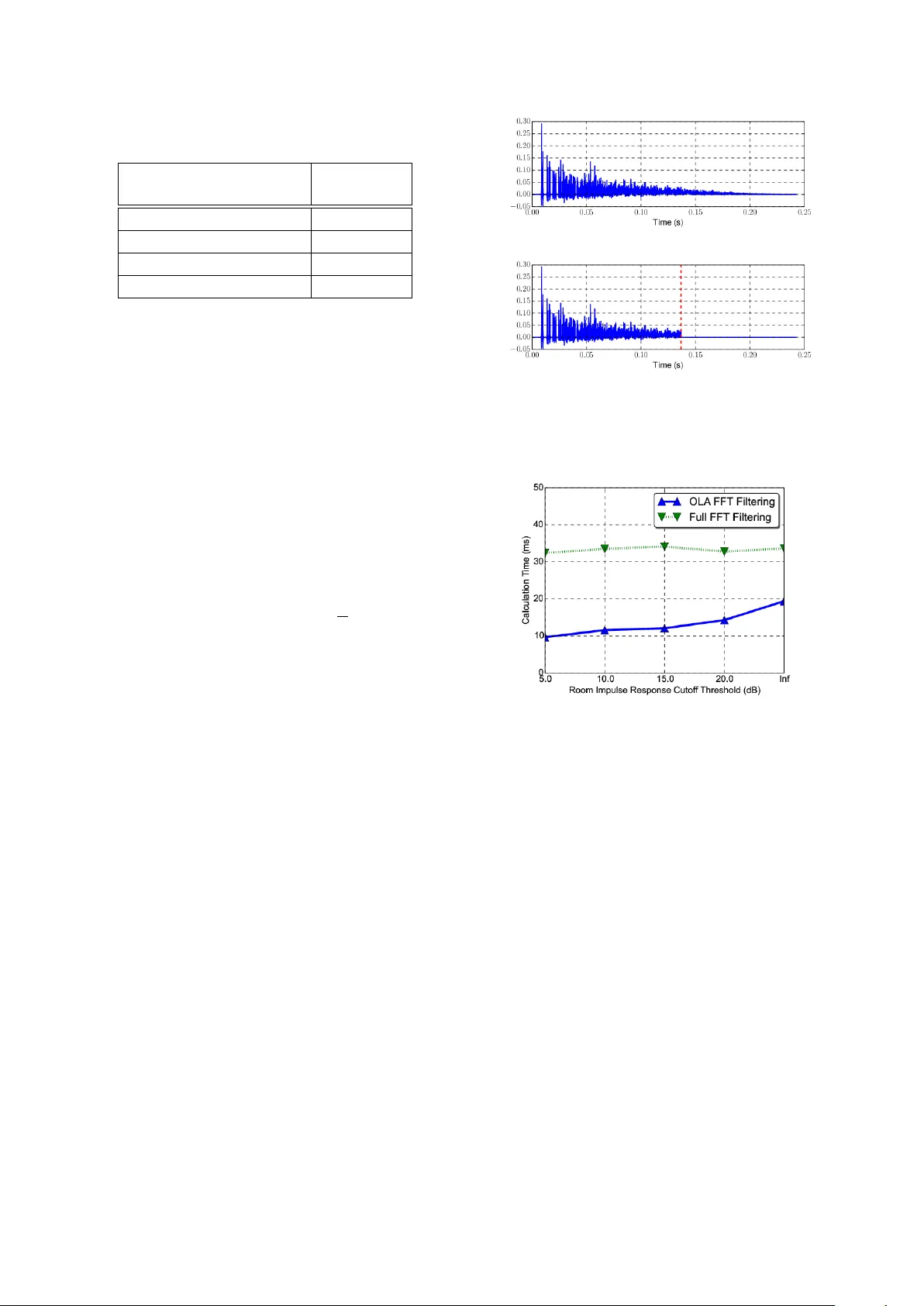
Efficient Implementation of the Room Simulator f or T raining Deep Neural Network Acoustic Models Chanwoo Kim 1 † , Ehsan V ariani 2 , Arun Narayanan 2 , and Michiel Bacc hiani 2 1 Samsung Research, 2 Google Speech 1 chanw.com@samsung.com 2 { variani, arunnt, michiel } @google.com Abstract In this paper , we describe how to ef ficiently implement an acoustic room simulator to generate large-scale simulated data for training deep neural networks. Even though Google Room Simulator in [1] w as sho wn to be quite ef fectiv e in reducing the W ord Error Rates (WERs) for far-field applications by gener- ating simulated far-field training sets, it requires a v ery large number of FFTs. Room Simulator used approximately 80 % of CPU usage in our CPU/GPU training architecture [2]. In this work, we implement an efficient OverLap Addition (OLA) based filtering using the open-source FFTW3 library . Further , we in vestigate the effects of the Room Impulse Response (RIR) lengths. Experimentally , we conclude that we can cut the tail portions of RIRs whose power is less than 20 dB belo w the maximum power without sacrificing the speech recognition ac- curacy . Ho wev er , we observe that cutting RIR tail more than this threshold harms the speech recognition accuracy for rere- corded test sets. Using these approaches, we were able to reduce CPU usage for the room simulator portion down to 9.69 % in CPU/GPU training architecture. Profiling result sho ws that we obtain 22.4 times speed-up on a single machine and 37.3 times speed up on Google’ s distributed training infrastructure. Index T erms : Simulated data, room acoustics, rob ust speech recognition, deep learning 1. Introduction W ith advancements in deep learning [3, 4, 5, 6, 7, 8], speech recognition accuracy has improved dramatically . Now , speech recognition systems are used not only on portable devices but also on standalone devices for far -field speech recognition. Ex- amples include voice assistant systems such as Amazon Ale xa and Google Home [1, 9]. In far -field speech recognition, the impact of noise and re verberation is much lar ger than near -field cases. T raditional approaches to f ar-field speech recognition in- clude noise robust feature extraction algorithms [10, 11, 12], on-set enhancement algorithms [13, 14], and multi-microphone approaches [15, 16, 17, 18, 19, 20, 21]. Recently , we observed that training with large-scale noisy data generated by a Room Simulator [1] improv es speech recognition accuracy dramati- cally . This system has been successfully employed for training acoustic models for Google Home or Google voice search [1]. Room Simulator creates millions of virtual rooms with dif- ferent dimensions and dif ferent number of sound sources at dif- ferent locations and Signal-to-Noise Ratios (SNRs). For e very new utterance in the training set, we use a randomly sampled room configuration, so that the same utterance is simulated un- der dif ferent acoustic en vironments in e very epoch during train- ing. As will be seen in Sec. 3, if we generate the simulated † W ork performed while at Google. GPU W orker Loss LSTM Stack F eatur e Extraction LSTM Stack P arameter Server (PS) Acoustic Simulation T raining W orker Queue f 1 , l 1 f N , l N Example Server Queue · · · ∂L ∂w 1 ∂L ∂w N · · · f 1 , l 1 f N , l N · · · Single Channel Input Batch ∂L ∂w 1 . . . ∂L ∂w N W ∆ W W CPU Room Configuration Generator Single or Multi-Channel Simulated Utterance Figure 1: T raining architecture using cluster of CPUs and GPUs. [2]. Room Simulator is on the CPU side to generate simulated utterances using room configurations. [1]. utterance only once for each input example, the performance is worse. Since different RIRs are applied for the same utter- ance at e very epoch, the intermediate results cannot be cached. Therefore, the noisification process requires very lar ge number of conv olution operations. As will be seen in Sec. 3, during training, Room Simulator used up to 80 % of the whole CPU usage if we use the CPU/GPU architecture shown in Fig. 1. In this paper , we describe our approach to reduce the computa- tional portion of the Room Simulator below 10 % of the CPU usage in our CPU/GPU training scheme. 2. Efficient Implementation of the Room Simulation System Fig. 1 sho ws a high level block diagram of the acoustic model training infrastructure [2]. Since it is not easy to run all the front-end processing blocks such as feature extraction and V oice Activity Detection (V AD) on GPUs, the y run on CPUs dur- ing training. Even though Fast Fourier Transform (FFT) of the Room Simulator may be efficiently implemented on GPUs, since Room Simulator must feed the simulated utterances to the rest of CPU optimized front-end components, the Room Simu- lator is also running on CPUs. 2.1. Review of the Room Simulator for Data A ugmentation In this section, we briefly re vie w the structure of the Google Room Simulator for generating simulated utterances to train acoustic models for speech recognition systems [1]. W e as- Figure 2: A simulated room: There may be multiple microphones, a single target sound source, multiple noise sources in a cuboid-shape room with acoustically reflectiv e walls [1]. sume a room of a rectangular cuboid-shape as sho wn in Fig. 2. Assuming that all the walls of a room reflect acoustically uniformly , we use the image method to model the Room Im- pulse Responses (RIRs) [22, 23, 24, 25]. In the image method, a real room is acoustically mirrored with respect to each wall, which results in grids of virtual rooms. In our work for train- ing the acoustic model for Google Home [1, 9], we consider 17 × 17 × 17 = 4913 virtual rooms for RIR calculation. Fol- lowing the image method and assuming that there are V virtual sound sources including one real source, the impulse response is calculated using the following equation [22, 23]: h [ n ] = V − 1 X v =0 r g v d v δ  n −  d v f s c 0  , (1) where v is the inde x of each virtual sound source, and d v > 0 is the distance from that sound source to the microphone, 0 < r < 1 is the reflection coef ficient of the wall, g v is the number of the reflections to that sound source, f s is the sampling rate of the RIR, and c 0 is the speed of sound in the air . W e use the v alue of f s = 16 , 000 Hz and c 0 = 343 m/s for Room Simulator [9]. For d v , r , we use numbers created by a random number generator following specified distrib utions for each impulse response [1]. Assuming that there are I sound sources including one tar- get source and J microphones, the receiv ed signal at micro- phone j is giv en by: y j [ n ] = I − 1 X i =0 α ij ( h ij [ n ] ∗ x i [ n ]) . (2) Since we used a tw o-microphones system in [1, 9] J is tw o, and for the number of noise sources, we used a value from zero up to three with an av erage of 1.55. Including the target source, the av erage number of I is 2.55 [1]. 2.2. Efficient Room Impulse Response filtering When the signal and the room impulse response lengths are N x and N h respectiv ely , the number of multiplications C td re- quired for calculating (2) using the time-domain conv olution is giv en by: C td = I × J × N x × N h . (3) In our training set used in [1, 9], the a verage utterance length in- cluding non-speec h portions marked by the V oice Acti vity De- tector (V AD) is 7.31 s . This corresponds to N x of 116,991 at 16 kHz . The a verage length of the RIR in the room simula- tor used in [1] is 0.243 s , corresponding to the N h value of 3893. For Google Home the number of noise sources in our training set is 1.55 on average. Thus I is 2.55 including one target source, and J is two, since we use a two-microphones system in [1, 9]. Thus, if we directly use the linear con volution, it requires 2.32 billion multiplications per utterance from (3), which is prohibitiv ely lar ge. Thus, in the “ Room Simulator ” in [1], we used the frequency domain multiplication using Kiss FFT [26]. T o av oid time aliasing, the FFT size N must satisfy N ≥ N x + M − 1 , where M is the length of the impulse re- sponse. The j -th microphone channel of the simulated signal y j [ n ] in (2) is giv en by: y j [ n ] = I − 1 X i =0 F F T − 1 { F F T { h ij [ n ] } × F F T { x i [ n ] }} . (4) As sho wn in (4), we perform tw o FFTs, one IFFT , and one com- plex element-wise multiplications between two complex spec- tra for each con volution term in (2). Assuming that radix-2 FFTs are employed, each FFT or IFFT requires N 2 log 2 ( N ) multiplications [27]. In addition, a single element-wise com- plex multiplication between two complex spectra is required for each con volution term in (2). For real time-domain sig- nals, we need to perform element-wise multiplications for the lower half-spectrum for Discrete Fourier Transform (DFT) in- dices 0 ≤ k ≤ N/ 2 since the spectrum has the Hermitian sym- metry property [27]. From this discussion, we conclude that the number of real multiplications C FFT for calculating (4) is giv en by: C FFT = I J (6 N log 2 ( N ) + 2 N ) . (5) For the average N x of 116,991 mentioned abov e, if we assume that the average N is 2 17 , (5) requires 69.5 million multiplica- tions per utterance on av erage. Room Simulator for [1, 9] was implemented in C++ using the Eigen3 linear algebra library [28]. So far we have used the Kiss FFT version of FFT in Eigen3 including acoustic model training for Google Home described in [1, 9]. But, to further speed up frontend computa- tion, we switched from Kiss FFT in Eigen3 to a custom C++ class implementation which internally uses real FFT in FFTW3 . A more ef ficient approach is using the Ov erLap Add (OLA) FFT filtering [27, 29]. W ith the OLA FFT filtering, the approx- imate number of real multiplications is giv en by: C OLA = I J  N x N − N h + 1  (4 N log 2 ( N ) + 2 N ) + 2 N log 2 ( N )  , (6) where N is the FFT size, N x is the length of the entire sig- nal, and N h is the length of the impulse response. The term 4 N log 2 ( N ) + 2 N appears in (6), since there is one FFT , one IFFT , and one element-wise comple x multiplication for 0 ≤ k ≤ N/ 2 for each block. As before, we assumed that each FFT or IFFT requires N 2 log 2 ( N ) multiplications and one complex multiplication requires four real multiplications in (6). j N x N − M +1 k is the number of blocks to process an utterance of length N x . The 2 N log 2 ( N ) term in (6) is required for FFT of the impulse response h ij [ n ] . For the impulse response h ij [ n ] , we do not T able 1: The profiling result for processing a single utterance using the “Room Simulator” on a local desktop machine A vg. Time per Utterance ( ms ) Original Room Simulator in [1] 320.8 ms FFTW3 Real FFT Filtering 44.2 ms +OLA filtering 19.4 ms +20 dB RIR cut-off 14.3 ms need to repeat it for ev ery block. In our training set consist- ing of 22 million utterances mentioned above, the a verage N is 116,991 and the average N h is 3,893. For this a verage N and N h , the minimum value of C OLA in (6) is 50.8 millions of real multiplications when N = 2 14 . The optimal value of N min- imizing C OLA is different for dif ferent N h and N x values. For each filtering, we minimize C OLA by ev aluating this equation with different v alues of N = 2 m where m is an integer . 2.3. Room Impulse Response Length Selection The a verage length of the Room Impulse Response in the origi- nal room simulator is estimated to be 3893 samples, which cor - responds to 0.243 s . W e perform a simple RIR tail-cutoff by finding the RIR po wer threshold which is η dB belo w the max- imum power of the RIR h ij [ n ] : p th = max  h 2 ij [ n ]  × 10 − η 10 . (7) Using p th , we find the cut-off index n c which is the smallest sample index beyond which all the trailing h ij [ n ] has po wer below the threshold p th : n c = min m  m     max n>m  h 2 [ n ]  < p th  . (8) Then the final RIR cut-of f b h ij [ n ] is given by the follo wing equa- tion: b h ij [ n ] = h ij [ n ] , 0 ≤ n ≤ n c + 1 . (9) Fig. 3 sho ws the original impulse responses and the correspond- ing RIR when the cutoff threshold of η is used. T o reflect the typical case in our training set, we used the average room di- mension, average microphone-to-target distance, and a verage T 60 value among 3 million room configurations described in [1]. As shown in T able 1 and 2, the RIR tail cut-off at 20 dB shows relativ ely 35.6 % to 69.4 % speed improvement on a lo- cal desktop machine and on Google Borg cluster [30]. Fig. 4 shows the profiling results on a local machine with different RIR cutof f thresholds η . The local machine we used has a single Intel(R) Xeon(R) E5-1650 @ 3.20GHz CPU with 6 cores and 32 GB of memory . In Fig. 4, we observe that the computational cost becomes less for the OLA filtering case as we cut the tail portion of the RIR more. For the full FFT case, theoretically , it should remain almost constant regardless of the impulse response length, but due to variation in profiling mea- surement, there is some small variation. (a) (b) Figure 3: The simulated room impulse responses generated in the “Room Simulator” described in Sec. 2: (a) The impulse response without the RIR tail cut-off, (b) with the RIR tail cut-off at 20 dB . Figure 4: Profiling result on local desktop machine with different RIR cut-of f threshold with and without OverLap Addition FIR filtering. 3. Experimental results In this section, we present speech recognition results and CPU profiling results obtained using Room Simulator with differ- ent RIR cut-of f thresholds. The acoustic modeling structure to obtain experimental results in this section is somewhat dif- ferent from those described in [1, 9] for f aster training. W e use a single-channel 128 log-Mel feature whose window size is 32 ms . The interval between successive frame is 10 ms . The low and upper cutoff frequencies of the Mel filterbank are 125 Hz and 7500 Hz respectively . Since it has been shown that long-duration features represented by overlapping features are helpful [31], four frames are stacked together . Thus we use a context dependent feature consisting of 512 elements giv en by 128 (the size of the log-mel feature) x 4 (number of stacked frames). This input is down-sampled by a factor of three [32]. The feature is processed by a typical multi-layer Long Short- T erm Memory (LSTM) [33, 34] acoustic model. W e use 5-layer LSTMs with 768 units in each layer . The output of the final LSTM layer is passed to a softmax layer . The softmax layer has 8192 nodes corresponding to the number of tied context- dependent phones in our ASR system. The output state label is delayed by five frames, since it was observed that the infor- mation about future frames improv es the prediction of the cur - T able 2: The CPU usage portion of the FFT and Room Simulator with the respect to the entire CPU pipeline in Fig. 1 and relativ e speed up measured in terms of ex ecution time with respect to our baseline in [1] on Google Borg cluster [30]. Original system in [1] FFTW3 OLA Filter FFTW3 OLA Filter with 20 dB RIR Cut-off FFTW3 OLA Filter with 10 dB RIR Cut-off FFT portion (%) 79.27 % 10.11 % 6.23 % 5.08 % Relativ e Speed Up in FFT Portion (%) - 34.0 times 57.6 times 59.6 times Entire Acoustic Simulation (%) 80.01 % 13.30 % 9.69 % 8.05 % Relativ e Speed Up in Acoustic Simulation Portion (%) - 26.1 times 37.3 times 45.7 times T able 3: Speech recognition experimental result in terms of W ord Error Rates (WERs) with and without MTR using the room simulation system in [1] and different RIR cutof f thresholds. Baseline without MTR MTR using One-time Batch Room Simulation Baseline (On-the-fly Room Simulation) 20 dB RIR Cut-off 10 dB RIR Cut-off 5 dB RIR Cut-off Original T est Set 11.70 % 12.07 % 11.95 % 11.43 % 10.75 % 11.20 % Simulated Noisy Set A 20.75 % 15.58 % 14.88 % 13.96 % 13.59 % 14.99 % Simulated Noisy Set B 50.78 % 22.47 % 20.64 % 19.58 % 21.37 % 28.27 % Device 1 52.56 % 22.39 % 21.69 % 21.35 % 23.20 % 29.53 % Device 2 51.59 % 22.12 % 21.62 % 21.26 % 22.90 % 29.39 % Device 3 54.89 % 23.42 % 22.29 % 22.86 % 26.47 % 36.71 % Device 3 (Noisy Condition) 72.09 % 36.21 % 35.88 % 35.83 % 39.99 % 51.11 % Device 3 (Multi-T alker Condition) 74.60 % 47.63 % 46.03 % 46.21 % 48.36 % 58.31 % T able 4: A verage T 60 T ime of the Simulated T raining Set and Simulated T est Sets A and B. Simulated T raining Set Simulated Noisy Set A Simulated Noisy Set B A verage T 60 (s) 0.482 s 0.167 s 0.479 s rent frame [35, 36]. The acoustic model was trained using the Cross-Entropy (CE) loss as the objective function, using pre- computed alignments for utterance as targets. T o obtain results in T able 3, we trained for about 45 epochs. For training, we used an anonymized and hand-transcribed 22-million English utterances (18,000-hr) set. The training set is the same as what we used in [1, 9]. For evaluation, we used around 15-hour of utterances (13,795 utterances) obtained from anonymized mo- bile voice search data. W e also generate noisy ev aluation sets from this relatively clean voice search data. W e use both simu- lated and rerecorded noisy sets. The a verage re verberation time in T 60 of the simulated training set and two simulated test sets are sho wn in T able 4. These two simulated test sets are named Simulated Noisy Set A and Simulated Noisy Set B respectiv ely . Since our objectiv e is deploying our speech recognition sys- tems on far-field standalone devices such as Google Home, we rerecorded these e valuation sets using the actual hardware in far -field en vironment. Note that the actual Google Home hard- ware has tw o microphones with microphone spacing of 7.1 cm. In our e xperiments in this section, we selected the first channel out of two channel data. Three different devices were used in rerecording, and each device was placed in fiv e different loca- tions in an actual room resembling a real living room. These devices are listed in T able 3 as “Device 1”, “Device 2”, and “Device 3”. As shown in T able 3, we observe that the RIR cut- off up to 20 dB threshold does not adversely affect the perfor- mance. Howev er , if we cut the RIR to 5 dB threshold, then the performance under far-field en vironment becomes significantly worse. This observation also confirms that far-field speech recog- nition benefits from RIRs with sufficiently long tails in the train- ing set. T able 2 shows how much CPU resource was used when training is done on Google Borg cluster [30] using the CPU/GPU training architecture in Fig. 1. W e observe that if we use the FFTW3 -based OLA filter using 20 dB RIR cutoff, we may ob- tain 57.6 times speed-up in the FFT portion. The entire speed- up of Room Simulator portion is 37.3 times. 4. Conclusions In this paper , we describe ho w to ef ficiently implement an acous- tic room simulator to generate lar ge-scale simulated data for training deep neural networks. W e implement an ef ficient Over - Lap Addition (OLA) based filtering using the open-source FFTW3 library . W e in vestigate into the ef fects of the Room Impulse Re- sponse (RIR) lengths. W e conclude that we can cut the tail por - tions of RIRs whose power is less than 20 dB below the max- imum power without sacrificing speech recognition accuracy . Howe ver , if we cut of f RIR more than that, we observe it ad- versely af fects the performance for re verberant cases. Using the approaches mentioned here, we could reduce the room simu- lator portion in the CPU usage do wn to 9.69 % in CPU/GPU training architecture. Profiling result sho ws that we obtain 22.4 times speed-up on a local desktop machine and 37.3 times speed up on Google Borg cluster . 5. References [1] C. Kim, A. Misra, K.K. Chin, T . Hughes, A. Narayanan, T . Sainath, and M. Bacchiani, “Generation of simulated utterances in virtual rooms to train deep-neural netw orks for far -field speech recognition in Google Home, ” in INTERSPEECH-2017 , Aug. 2017, pp. 379–383. [2] E. V ariani, T . Bagby , E. McDermott, and M. Bacchiani, “End-to- end training of acoustic models for large vocabulary continuous speech recognition with tensorflow, ” in INTERSPEECH-2017 , 2017, pp. 1641–1645. [Online]. A vailable: http://dx.doi.org/10. 21437/Interspeech.2017- 1284 [3] M. Seltzer , D. Y u, and Y .-Q. W ang, “ An in vestigation of deep neu- ral networks for noise robust speech recognition, ” in Int. Conf. Acoust. Speech, and Signal Pr ocessing , 2013, pp. 7398–7402. [4] D. Y u, M. L. Seltzer, J. Li, J.-T . Huang, and F . Seide, “Feature learning in deep neural networks - studies on speech recognition tasks, ” in Proceedings of the International Conference on Learn- ing Repr esentations , 2013. [5] V . V anhoucke, A. Senior , and M. Z. Mao, “Impro ving the speed of neural networks on CPUs, ” in Deep Learning and Unsupervised F eature Learning NIPS W orkshop , 2011. [6] G. Hinton, L. Deng, D. Y u, G. E. Dahl, A. Mohamed, N. Jaitly , A. Senior , V . V anhoucke, P . Nguyen, T . Sainath, and B. Kingsbury , “Deep neural networks for acoustic modeling in speech recog- nition: The shared views of four research groups, ” IEEE Signal Pr ocessing Magazine , vol. 29, no. 6, No v . [7] T . Sainath, R. J. W eiss, K. W . Wilson, B. Li, A. Narayanan, E. V ariani, M. Bacchiani, I. Shafran, A. Senior, K. Chin, A. Misra, and C. Kim, “Multichannel signal processing with deep neural networks for automatic speech recognition, ” IEEE/ACM T rans. Audio, Speec h, Lang. Pr ocess. , Feb . 2017. [8] ——, “Raw Multichannel Processing Using Deep Neural Net- works, ” in New Era for Robust Speech Recognition: Exploiting Deep Learning , S. W atanabe, M. Delcroix, F . Metze, and J. R. Hershey , Ed. Springer , Oct. 2017. [9] B. Li, T . Sainath, A. Narayanan, J. Caroselli, M. Bacchiani, A. Misra, I. Shafran, H. Sak, G. Pundak, K. Chin, K-C Sim, R. W eiss, K. Wilson, E. V ariani, C. Kim, O. Siohan, M. W eintraub, E. McDermott, R. Rose, and M. Shannon, “ Acoustic modeling for Google Home, ” in INTERSPEECH-2017 , Aug. 2017, pp. 399– 403. [10] C. Kim and R. M. Stern, “Po wer-Normalized Cepstral Coef- ficients (PNCC) for Robust Speech Recognition, ” IEEE/ACM T rans. A udio, Speech, Lang. Pr ocess. , pp. 1315–1329, July 2016. [11] U. H. Y apanel and J. H. L. Hansen, “A new perceptually motiv ated MVDR-based acoustic front-end (PMVDR) for robust automatic speech recognition, ” Speech Communication , vol. 50, no. 2, pp. 142–152, Feb . 2008. [12] C. Kim and R. M. Stern, “Feature extraction for robust speech recognition based on maximizing the sharpness of the power dis- tribution and on po wer flooring, ” in IEEE Int. Conf. on Acoustics, Speech, and Signal Pr ocessing , March 2010, pp. 4574–4577. [13] ——, “Nonlinear enhancement of onset for robust speech recog- nition, ” in INTERSPEECH-2010 , Sept. 2010, pp. 2058–2061. [14] C. Kim, K. Chin, M. Bacchiani, and R. M. Stern, “Robust speech recognition using temporal masking and thresholding algorithm, ” in INTERSPEECH-2014 , Sept. 2014, pp. 2734–2738. [15] T . Nakatani, N. Ito, T . Higuchi, S. Araki, and K. Kinoshita, “In- tegrating DNN-based and spatial clustering-based mask estima- tion for robust MVDR beamforming, ” in IEEE Int. Conf. Acoust., Speech, Signal Pr ocessing , March 2017, pp. 286–290. [16] T . Higuchi and N. Ito and T . Y oshioka and T . Nakatani, “Ro- bust MVDR beamforming using time-frequency masks for on- line/offline ASR in noise, ” in IEEE Int. Conf. Acoust., Speech, Signal Pr ocessing , March 2016, pp. 5210–5214. [17] H. Erdogan, J. R. Hershey , S. W atanabe, M. Mandel, J. Roux, “Improved MVDR Beamforming Using Single-Channel Mask Prediction Networks, ” in INTERSPEECH-2016 , Sept 2016, pp. 1981–1985. [18] C. Kim and K. K. Chin, “Sound source separation algorithm using phase difference and angle distribution modeling near the target, ” in INTERSPEECH-2015 , Sept. 2015, pp. 751–755. [19] C. Kim, K. Kumar , B. Raj, and R. M. Stern, “Signal separation for robust speech recognition based on phase difference informa- tion obtained in the frequenc y domain, ” in INTERSPEECH-2009 , Sept. 2009, pp. 2495–2498. [20] C. Kim, C. Khawand, and R. M. Stern, “T wo-microphone source separation algorithm based on statistical modeling of angle dis- tributions, ” in IEEE Int. Conf. on Acoustics, Speech, and Signal Pr ocessing , March 2012, pp. 4629–4632. [21] C. Kim, K. Kumar, and R. M. Stern, “Binaural sound source sep- aration motiv ated by auditory processing, ” in IEEE Int. Conf. on Acoustics, Speec h, and Signal Processing , May 2011, pp. 5072– 5075. [22] J. Allen and D. Berkley , “Image method for ef ficiently simulating small-room acoustics, ” J. Acoust. Soc. Am. , vol. 65, no. 4, pp. 943–950, April 1979. [23] E. A. Lehmann, A. M. Johansson, and S. Nordholm, “Rev erberation-time prediction method for room impulse re- sponses simulated with the image-source model, ” in 2007 IEEE W orkshop on Applications of Signal Processing to Audio and Acoustics , Oct. 2007, pp. 159–162. [24] S. G. McGov ern. room impulse response generator . [On- line]. A vailable: https://www .mathworks.com/matlabcentral/ fileexchange/5116- room- impulse- response- generator [25] ——, “Fast image method for impulse response calculations of box-shaped rooms, ” Applied Acoustics , vol. 70, no. 1, pp. 182 – 189, 2009. [26] M. Borgerding, “Kiss f ft version 1.2.9, ” https://sourceforge.net/projects/kissf ft/, 2010. [27] A. V . Oppenheim and R. W .Scafer , with .J. R. Buck, Discrete-time Signal Pr ocessing , 2nd ed. Englew ood-Cliffs, NJ: Prentice-Hall, 1998. [28] G. Guennebaud, B. Jacob et al., “Eigen v3, ” http://eigen.tuxfamily .org, 2010. [29] R. Crochiere, “A weighted overlap-add method of short-time Fourier analysis/synthesis, ” IEEE T rans. Acoust., Speech, and Signal Pr ocessing , vol. 28, no. 1, pp. 99–102, feb 1980. [30] A. V erma, L. Pedrosa, M. R. K orupolu, D. Oppenheimer, E. T une, and J. W ilkes, “Large-scale cluster management at Google with Borg, ” in Proceedings of the European Conference on Computer Systems (Eur oSys) , Bordeaux, France, 2015. [31] H. Sak, A. Senior , K. Rao, and F . Beaufays, “Fast and Accurate Recurrent Neural Network Acoustic Models for Speech Recogni- tion, ” in INTERSPEECH-2015 , Sept. 2015, pp. 1468–1472. [32] G. Pundak and T . N. Sainath, “Lower Frame Rate Neural Network Acoustic Models, ” 2016, pp. 22–26. [Online]. A vailable: http://dx.doi.org/10.21437/Interspeech.2016- 275 [33] S. Hochreiter and J ¨ urgen Schmidhuber , “Long Short-term Mem- ory , ” Neural Computation , no. 9, pp. 1735–1780, Nov . 1997. [34] T . N. Sainath, O. Vin yals, A. Senior, and H. Sak, “Conv olutional, long short-term memory , fully connected deep neural networks, ” in IEEE Int. Conf. Acoust., Speech and Signal Pr ocessing , Apr . 2015, pp. 4580–4584. [35] H. Sak, A. Senior , and F . Beauf ays, “Long short-term memory re- current neural network architectures for large scale acoustic mod- eling, ” in INTERSPEECH-2014 , Sept. 2014, pp. 338–342. [36] M. Schuster and K. P aliwal, “Bidirectional recurrent neural net- works, ” IEEE Tr ansactions on Signal Processing , v ol. 45, no. 11, pp. 2673–2681, 1997.