Feature Learning in Deep Neural Networks - Studies on Speech Recognition Tasks

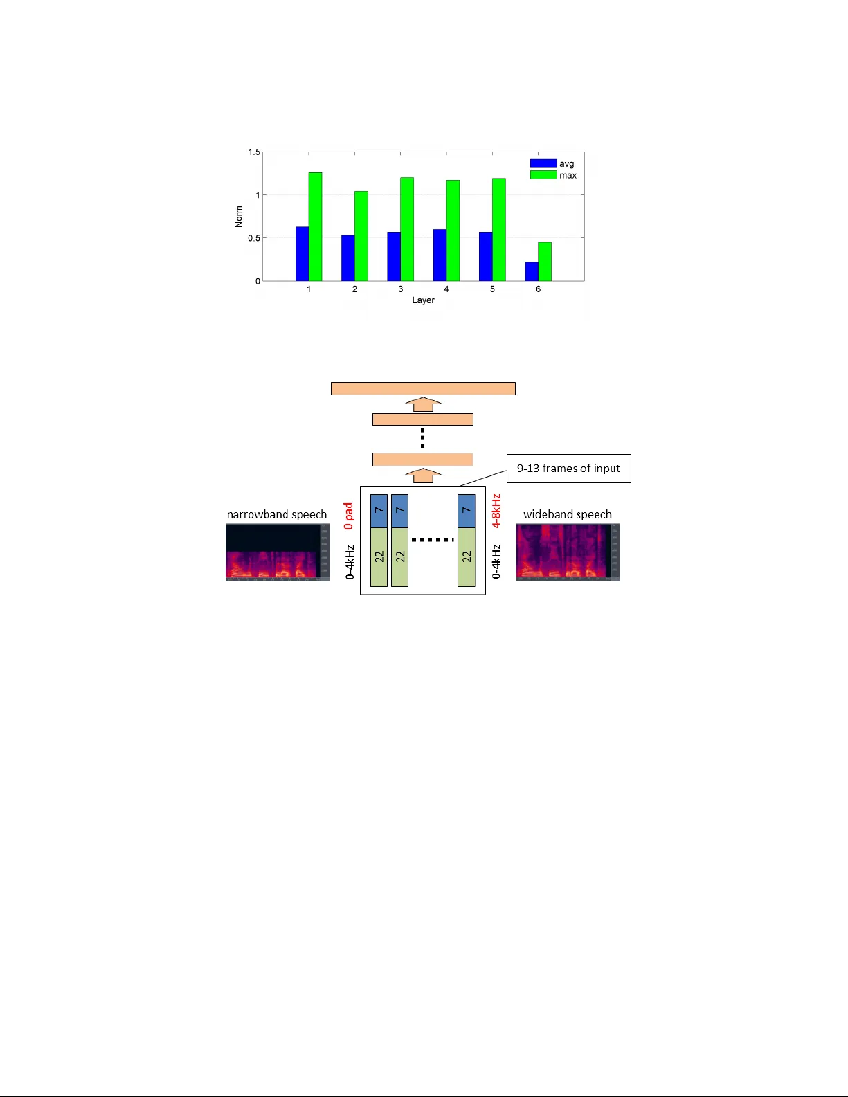
F eatur e Lear ning in Deep Neural Networks – Studies on Speech Recognition T asks Dong Y u, Michael L. Seltzer , Jinyu Li 1 , Jui-T ing Huang 1 , Frank Seide 2 Microsoft Research, Redmond, W A 98052 1 Microsoft Corporation, Redmond, W A 98052 2 Microsoft Research Asia, Beijing, P .R.C. { dongyu,mseltzer,jinyli,jthuang,fseide } @microsoft.com Abstract Recent studies hav e shown that deep neural netw orks (DNNs) perform signifi- cantly better than shallo w networks and Gaussian mixture models (GMMs) on large v ocabulary speech recognition tasks. In this paper , we argue that the im- prov ed accuracy achieved by the DNNs is the result of their ability to extract dis- criminativ e internal representations that are rob ust to the many sources of v ariabil- ity in speech signals. W e show that these representations become increasingly in- sensitiv e to small perturbations in the input with increasing network depth, which leads to better speech recognition performance with deeper networks. W e also show that DNNs cannot extrapolate to test samples that are substantially dif fer- ent from the training examples. If the training data are sufficiently representati ve, howe ver , internal features learned by the DNN are relativ ely stable with respect to speaker dif ferences, bandwidth dif ferences, and environment distortion. This enables DNN-based recognizers to perform as well or better than state-of-the-art systems based on GMMs or shallo w networks without the need for e xplicit model adaptation or feature normalization. 1 Introduction Automatic speech recognition (ASR) has been an activ e research area for more than five decades. Howe ver , the performance of ASR systems is still far from satisfactory and the gap between ASR and human speech recognition is still large on most tasks. One of the primary reasons speech recognition is challenging is the high v ariability in speech signals. For example, speakers may hav e dif ferent accents, dialects, or pronunciations, and speak in different styles, at different rates, and in different emotional states. The presence of environmental noise, rev erberation, different microphones and recording devices results in additional variability . T o complicate matters, the sources of variability are often nonstationary and interact with the speech signal in a nonlinear way . As a result, it is virtually impossible to av oid some degree of mismatch between the training and testing conditions. Con ventional speech recognizers use a hidden Markov model (HMM) in which each acoustic state is modeled by a Gaussian mixture model (GMM). The model parameters can be discriminativ ely trained using an objectiv e function such as maximum mutual information (MMI) [1] or minimum phone error rate (MPE) [2]. Such systems are known to be susceptible to performance degrada- tion when ev en mild mismatch between training and testing conditions is encountered. T o combat this, a variety of techniques has been de veloped. For example, mismatch due to speaker differ - ences can be reduced by V ocal T ract Length Normalization (VTLN) [3], which nonlinearly warps the input feature vectors to better match the acoustic model, or Maximum Likelihood Linear Re- gression (MLLR) [4], which adapt the GMM parameters to be more representative of the test data. Other techniques such as V ector T aylor Series (VTS) adaptation are designed to address the mis- match caused by en vironmental noise and channel distortion [5]. While these methods hav e been 1 successful to some degree, they add complexity and latency to the decoding process. Most require multiple iterations of decoding and some only perform well with ample adaptation data, making them unsuitable for systems that process short utterances, such as voice search. Recently , an alternativ e acoustic model based on deep neural networks (DNNs) has been proposed. In this model, a collection of Gaussian mixture models is replaced by a single context-dependent deep neural network (CD-DNN). A number of research groups ha ve obtained strong results on a variety of lar ge scale speech tasks using this approach [6 – 13]. Because the temporal structure of the HMM is maintained, we refer to these models as CD-DNN-HMM acoustic models. In this paper , we analyze the performance of DNNs for speech recognition and in particular , exam- ine their ability to learn representations that are robust to v ariability in the acoustic signal. T o do so, we interpret the DNN as a joint model combining a nonlinear feature transformation and a log- linear classifier . Using this view , we show that the many layers of nonlinear transforms in a DNN con vert the raw features into a highly inv ariant and discriminativ e representation which can then be effecti vely classified using a log-linear model. These internal representations become increasingly insensitiv e to small perturbations in the input with increasing netw ork depth. In addition, the classi- fication accuracy impro ves with deeper networks, although the gain per layer diminishes. Howe ver , we also find that DNNs are unable to e xtrapolate to test samples that are substantially dif ferent from the training samples. A series of experiments demonstrates that if the training data are suf ficiently representativ e, the DNN learns internal features that are relativ ely in variant to sources of v ariability common in speech recognition such as speaker differences and en vironmental distortions. This en- ables DNN-based speech recognizers to perform as well or better than state-of-the-art GMM-based systems without the need for explicit model adaptation or feature normalization algorithms. The rest of the paper is organized as follows. In Section 2 we briefly describe DNNs and illustrate the feature learning interpretation of DNNs. In Section 3 we show that DNNs can learn in variant and discriminativ e features and demonstrate empirically that higher layer features are less sensitive to perturbations of the input. In Section 4 we point out that the feature generalization ability is effecti ve only when test samples are small perturbations of training samples. Otherwise, DNNs perform poorly as indicated in our mix ed-bandwidth experiments. W e apply this analysis to speak er adaptation in Section 5 and find that deep networks learn speaker -inv ariant representations, and to the Aurora 4 noise robustness task in Section 6 where we sho w that a DNN can achieve performance equiv alent to the current state of the art without requiring e xplicit adaptation to the en vironment. W e conclude the paper in Section 7. 2 Deep Neural Networks A deep neural network (DNN) is con ventional multi-layer perceptron (MLP) with many hidden layers (thus deep). If the input and output of the DNN are denoted as x and y , respectiv ely , a DNN can be interpreted as a directed graphical model that approximates the posterior probability p y | x ( y = s | x ) of a class s gi ven an observation vector x , as a stack of ( L + 1) layers of log-linear models. The first L layers model the posterior probabilities of hidden binary vectors h ` giv en input vectors v ` . If h ` consists of N ` hidden units, each denoted as h ` j , the posterior probability can be expressed as p ` ( h ` | v ` ) = N ` Y j =1 e z ` j ( v ` ) · h ` j e z ` j ( v ` ) · 1 + e z ` j ( v ` ) · 0 , 0 ≤ ` < L where z ` ( v ` ) = ( W ` ) T v ` + a ` , and W ` and a ` represent the weight matrix and bias vector in the ` -th layer , respectively . Each observation is propagated forward through the network, starting with the lo west layer ( v 0 = x ) . The output variables of each layer become the input v ariables of the next, i.e. v ` +1 = h ` . In the final layer, the class posterior probabilities are computed as a multinomial distribution p y | x ( y = s | x ) = p L ( y = s | v L ) = e z L s ( v L ) P s 0 e z L s 0 ( v L ) = softmax s  v L  . (1) Note that the equality between p y | x ( y = s | x ) and p L ( y = s | v L ) is valid by making a mean-field approximation [14] at each hidden layer . 2 In the DNN, the estimation of the posterior probability p y | x ( y = s | x ) can also be considered a two- step deterministic process. In the first step, the observation vector x is transformed to another feature vector v L through L layers of non-linear transforms.In the second step, the posterior probability p y | x ( y = s | x ) is estimated using the log-linear model (1) giv en the transformed feature vector v L . If we consider the first L layers fixed, learning the parameters in the softmax layer is equiv alent to training a conditional maximum-entropy (MaxEnt) model on features v L . In the con ventional MaxEnt model, features are manually designed [15]. In DNNs, howe ver , the feature representations are jointly learned with the MaxEnt model from the data. This not only eliminates the tedious and potentially erroneous process of manual feature extraction but also has the potential to automatically extract in v ariant and discriminativ e features, which are difficult to construct manually . In all the following discussions, we use DNNs in the framework of the CD-DNN-HMM [6–10] and use speech recognition as our classification task. The detailed training procedure and decoding technique for CD-DNN-HMMs can be found in [6 – 8]. 3 In variant and discriminative features 3.1 Deeper is better Using DNNs instead of shallow MLPs is a key component to the success of CD-DNN-HMMs. T a- ble 1, which is extracted from [8], summarizes the word error rates (WER) on the Switchboard (SWB) [16] Hub5’00-SWB test set. Switchboard is a corpus of con versational telephone speech. The system was trained using the 309-hour training set with labels generated by V iterbi align- ment from a maximum likelihood (ML) trained GMM-HMM system. The labels correspond to tied-parameter context-dependent acoustic states called senones. Our baseline WER with the cor- responding discriminatively trained traditional GMM-HMM system is 23.6%, while the best CD- DNN-HMM achi ves 17.0%—a 28% relativ e error reduction (it is possible to further improv e the DNN to a one-third reduction by realignment [8]). W e can observe that deeper networks outperform shallow ones. The WER decreases as the number of hidden layers increases, using a fixed layer size of 2048 hidden units. In other words, deeper mod- els have stronger discriminativ e ability than shallow models. This is also reflected in the improve- ment of the training criterion (not shown). More interestingly , if architectures with an equiv alent number of parameters are compared, the deep models consistently outperform the shallow models when the deep model is suf ficiently wide at each layer . This is reflected in the right column of the table, which shows the performance for shallow networks with the same number of parameters as the deep networks in the left column. Even if we further increase the size of an MLP with a single hidden layer to about 16000 hidden units we can only achiev e a WER of 22.1%, which is signifi- cantly worse than the 17.1% WER that is obtained using a 7 × 2 k DNN under the same conditions. Note that as the number of hidden layers further increases, only limited additional gains are obtained and performance saturates after 9 hidden layers. The 9x2k DNN performs equally well as a 5x3k DNN which has more parameters. In practice, a tradeoff needs to be made between the width of each layer , the additional reduction in WER and the increased cost of training and decoding as the number of hidden layers is increased. 3.2 DNNs learn more in variant features W e have noticed that the biggest benefit of using DNNs over shallo w models is that DNNs learn more in variant and discriminative features. This is because many layers of simple nonlinear processing can generate a complicated nonlinear transform. T o show that this nonlinear transform is robust to small v ariations in the input features, let’ s assume the output of layer l − 1 , or equi v alently the input to the layer l is changed from v ` to v ` + δ ` , where δ ` is a small change. This change will cause the output of layer l , or equiv alently the input to the layer ` + 1 to change by δ ` +1 = σ ( z ` ( v ` + δ ` )) − σ ( z ` ( v ` )) ≈ diag  σ 0 ( z ` ( v ` ))  ( w ` ) T δ ` . 3 T able 1: Effect of CD-DNN-HMM network depth on WER (%) on Hub5’00-SWB using the 309- hour Switchboard training set. DBN pretraining is applied. L × N WER 1 × N WER 1 × 2 k 24.2 – – 2 × 2 k 20.4 – – 3 × 2 k 18.4 – – 4 × 2 k 17.8 – – 5 × 2 k 17.2 1 × 3772 22.5 7 × 2 k 17.1 1 × 4634 22.6 9 × 2 k 17.0 – – 5 × 3 k 17.0 – – – – 1 × 16 k 22.1 Figure 1: Percentage of saturated activ ations at each layer The norm of the change δ ` +1 is k δ ` +1 k ≈ k diag ( σ 0 ( z ` ( v ` )))(( w ` ) T δ ` ) k ≤ k diag ( σ 0 ( z ` ( v ` )))( w ` ) T kk δ ` k = k diag ( v ` +1 ◦ (1 − v ` +1 ))( w ` ) T kk δ ` k (2) where ◦ refers to an element-wise product. Note that the magnitude of the majority of the weights is typically very small if the size of the hidden layer is large. For example, in a 6 × 2 k DNN trained using 30 hours of SWB data, 98% of the weights in all layers except the input layer ha ve magnitudes less than 0.5. While each element in v ` +1 ◦ (1 − v ` +1 ) is less than or equal to 0.25, the actual value is typically much smaller . This means that a large percentage of hidden neurons will not be active, as shown in Figure 1. As a result, the a verage norm k diag ( v ` +1 ◦ (1 − v ` +1 ))( w ` ) T k 2 in (2) across a 6-hr SWB dev elopment set is smaller than one in all layers, as indicated in Figure 2. Since all hidden layer values are bounded in the same range of (0 , 1) , this indicates that when there is a small perturbation on the input, the perturbation shrinks at each higher hidden layer . In other w ords, features generated by higher hidden layers are more inv ariant to variations than those represented by lower layers. Note that the maximum norm over the same development set is larger than one, as seen in Figure 2. This is necessary since the differences need to be enlarged around the class boundaries to have discrimination ability . 4 Learning by seeing In Section 3, we showed empirically that small perturbations in the input will be gradually shrunk as we move to the internal representation in the higher layers. In this section, we point out that the 4 Figure 2: A verage and maximum k diag ( v ` +1 ◦ (1 − v ` +1 ))( w ` ) T k 2 across layers on a 6 × 2 k DNN Figure 3: Illustration of mixed-bandwidth speech recognition using a DNN abov e result is only applicable to small perturbations around the training samples. When the test samples deviate significantly from the training samples, DNNs cannot accurately classify them. In other words, DNNs must see examples of representativ e variations in the data during training in order to generalize to similar variations in the test data. W e demonstrate this point using a mixed-bandwidth ASR study . T ypical speech recognizers are trained on either narro wband speech signals, recorded at 8 kHz, or wideband speech signals, recorded at 16 kHz. It would be advantageous if a single system could recognize both narrow- band and wideband speech, i.e. mixed-bandwidth ASR. One such system was recently proposed using a CD-DNN-HMM [17]. In that work, the follo wing DNN architecture was used for all experi- ments. The input features were 29 mel-scale log filter -bank outputs together with dynamic features. An 11-frame context window was used generating an input layer with 29 · 3 · 11 = 957 nodes. The DNN has 7 hidden layers, each with 2048 nodes. The output layer has 1803 nodes, corresponding to the number of senones determined by the GMM system. The 29-dimensional filter bank has two parts: the first 22 filters span 0–4 kHz and the last 7 filters span 4–8 kHz, with the center frequency of the first filter in the higher filter bank at 4 kHz. When the speech is wideband, all 29 filters hav e observed values. Ho wev er , when the speech is narrowband, the high-frequenc y information was not captured so the final 7 filters are set to 0. Figure 3 illustrates the architecture of the mixed-bandwidth ASR system. Experiments were conducted on a mobile voice search (VS) corpus. This task consists of internet search queries made by v oice on a smartphone.There are two training sets, VS-1 and VS-2, con- sisting of 72 and 197 hours of wideband audio data, respecti vely . These sets were collected during 5 T able 2: WER (%) on wideband (16k) and narrowband (8k) test sets with and without narrowband training data. training data 16 kHz VS-T 8 kHz VS-T 16 kHz VS-1 + 16 kHz VS-2 27.5 53.5 16 kHz VS-1 + 8 kHz VS-2 28.3 29.3 different times of year . The test set, called VS-T , has 26757 words in 9562 utterances. The narrow band training and test data were obtained by downsampling the wideband data. T able 2 summarizes the WER on the wideband and narrowband test sets when the DNN is trained with and without narrowband speech. From this table, it is clear that if all training data are wideband, the DNN performs well on the wideband test set (27.5% WER) but very poorly on the narrowband test set (53.5% WER). Ho we ver , if we con vert VS-2 to narro wband speech and train the same DNN using mixed-bandwidth data (second ro w), the DNN performs very well on both wideband and narrowband speech. T o understand the dif ference between these two scenarios, we take the output vectors at each layer for the wideband and narrowband input feature pairs, h ` ( x wb ) and h ` ( x nb ) , and measure their Eu- clidean distance. For the top layer , whose output is the senone posterior probability , we calculate the KL-div ergence in nats between p y | x ( s j | x wb ) and p y | x ( s j | x nb ) . T able 3 shows the statistics of d l and d y ov er 40 , 000 frames randomly sampled from the test set for the DNN trained using wideband speech only and the DNN trained using mixed-bandwidth speech. T able 3: Euclidean distance for the output vectors at each hidden layer (L1-L7) and the KL di- ver gence (nats) for the posteriors at the top layer between the narrowband (8 kHz) and wideband (16 kHz) input features, measured using the wideband DNN or the mixed-bandwidth DNN. wideband DNN mixed-band DNN layer dist mean variance mean variance L1 Eucl 13.28 3.90 7.32 3.62 L2 10.38 2.47 5.39 1.28 L3 8.04 1.77 4.49 1.27 L4 8.53 2.33 4.74 1.85 L5 9.01 2.96 5.39 2.30 L6 8.46 2.60 4.75 1.57 L7 5.27 1.85 3.12 0.93 T op KL 2.03 – 0.22 – From T able 3 we can observe that in both DNNs, the distance between hidden layer vectors generated from the wideband and narrowband input feature pair is significantly reduced at the layers close to the output layer compared to that in the first hidden layer . Perhaps what is more interesting is that the av erage distances and variances in the data-mixed DNN are consistently smaller than those in the DNN trained on wideband speech only . This indicates that by using mixed-bandwidth training data, the DNN learns to consider the differences in the wideband and narrowband input features as irrelev ant variations. These variations are suppressed after many layers of nonlinear transformation. The final representation is thus more inv ariant to this variation and yet still has the ability to distinguish between dif ferent class labels. This beha vior is ev en more obvious at the output layer since the KL-diver gence between the paired outputs is only 0.22 in the mixed-bandwidth DNN, much smaller than the 2.03 observed in the wideband DNN. 5 Robustness to speaker variation A major source of v ariability is variation across speak ers. T echniques for adapting a GMM-HMM to a speaker hav e been in v estigated for decades. T w o important techniques are VTLN [3], and feature- space MLLR (fMLLR) [4]. Both VTLN and fMLLR operate on the features directly , making their application in the DNN context straightforward. 6 T able 4: Comparison of feature-transform based speaker-adaptation techniques for GMM-HMMs, a shallo w , and a deep NN. W ord-error rates in % for Hub5’00-SWB (relativ e change in parentheses). GMM-HMM CD-MLP-HMM CD-DNN-HMM adaptation technique 40 mix 1 × 2k 7 × 2k speaker independent 23.6 24.2 17.1 + VTLN 21.5 (-9%) 22.5 (-7%) 16.8 (-2%) + { fMLLR/fDLR }× 4 20.4 (-5%) 21.5 (-4%) 16.4 (-2%) VTLN warps the frequency axis of the filterbank analysis to account for the fact that the precise lo- cations of vocal-tract resonances vary roughly monotonically with the physical size of the speaker . This is done in both training and testing. On the other hand, fMLLR applies an affine transform to the feature frames such that an adaptation data set better matches the model. In most cases, in- cluding this work, ‘self-adaptation’ is used: generate labels using unsupervised transcription, then re-recognize with the adapted model. This process is iterated four times. For GMM-HMMs, fM- LLR transforms are estimated to maximize the likelihood of the adaptation data given the model. For DNNs, we instead maximize cross entropy (with back propagation), which is a discriminative criterion, so we prefer to call this transform feature-space Discriminati ve Linear Re gression (fDLR). Note that the transform is applied to individual frames, prior to concatenation. T ypically , applying VTLN and fMLLR jointly to a GMM-HMM system will reduce errors by 10– 15%. Initially , similar gains were expected for DNNs as well. Howe ver , these gains were not realized, as shown in T able 4 [9]. The table compares VTLN and fMLLR/fDLR for GMM-HMMs, a context-dependent ANN-HMM with a single hidden layer , and a deep network with 7 hidden layers, on the same Switchboard task described in Section 3.1. For this task, test data are very consistent with the training, and thus, only a small amount of adaptation to other factors such as recording conditions or environmental factors occurs. W e use the same configuration as in T able 1 which is speaker independent using single-pass decoding. For the GMM-HMM, VTLN achie ves a strong relati ve gain of 9%. VTLN is also effecti ve with the shallow neural-network system, gaining a slightly smaller 7%. Howe ver , the impro vement of VTLN on the deep network with 7 hidden layers is a much smaller 2% gain. Combining VTLN with fDLR further reduces WER by 5% and 4% relativ e, for the GMM-HMM and the shallow network, respectiv ely . The reduction for the DNN is only 2%. W e also tried transplanting VTLN and fMLLR transforms estimated on the GMM system into the DNN, and achiev ed very similar results [9]. The VTLN and fDLR implementations of the shallo w and deep networks are identical. Thus, we conclude that to a significant de gree, the deep neural network is able to learn internal representations that are in variant with respect to the sources of v ariability that VTLN and fDLR address. 6 Robustness to en vir onmental distortions In many speech recognition tasks, there are often cases where the despite the presence of variability in the training data, significant mismatch between training and test data persists. En vironmental factors are common sources of such mismatch, e.g. ambient noise, reverberation, microphone type and capture device. The analysis in the previous sections suggests that DNNs have the ability to generate internal representations that are robust with respect to variability seen in the training data. In this section, we ev aluate the extent to which this in v ariance can be obtained with respect to distortions caused by the en vironment. W e performed a series of experiments on the Aurora 4 corpus [18], a 5000-word vocabulary task based on the W all Street Journal (WSJ0) corpus. The experiments were performed with the 16 kHz multi-condition training set consisting of 7137 utterances from 83 speakers. One half of the ut- terances was recorded by a high-quality close-talking microphone and the other half was recorded using one of 18 dif ferent secondary microphones. Both halves include a combination of clean speech and speech corrupted by one of six different types of noise (street traf fic, train station, car , babble, restaurant, airport) at a range of signal-to-noise ratios (SNR) between 10-20 dB. 7 The e valuation set consists of 330 utterances from 8 speakers. This test set was recorded by the pri- mary microphone and a number of secondary microphones. These two sets are then each corrupted by the same six noises used in the training set at SNRs between 5-15 dB, creating a total of 14 test sets. These 14 test sets can then be grouped into 4 subsets, based on the type of distortion: none (clean speech), additi ve noise only , channel distortion only , and noise + channel. Notice that the types of noise are common across training and test sets but the SNRs of the data are not. The DNN was trained using 24-dimensional log mel filterbank features with utterance-lev el mean normalization. The first- and second-order deri vati ve features were appended to the static feature vectors. The input layer was formed from a context window of 11 frames creating an input layer of 792 input units. The DNN had 7 hidden layers with 2048 hidden units in each layer and the final softmax output layer had 3206 units, corresponding to the senones of the baseline HMM system. The network was initialized using layer-by-layer generativ e pre-training and then discriminatively trained using back propagation. In T able 5, the performance obtained by the DNN acoustic model is compared to se veral other systems. The first system is a baseline GMM-HMM system, while the remaining systems are repre- sentativ e of the state of the art in acoustic modeling and noise and speaker adaptation. All used the same training set. T o the authors’ knowledge, these are the best published results on this task. The second system combines Minimum Phone Error (MPE) discriminati ve training [2] and noise adaptiv e training (N A T) [19] using VTS adaptation to compensate for noise and channel mismatch [20]. The third system uses a hybrid generati ve/discriminati ve classifier [21] as follows . First, an adaptiv ely trained HMM with VTS adaptation is used to generate features based on state lik elihoods and their deriv ati ves. Then, these features are input to a discriminativ e log-linear model to obtain the final hypothesis. The fourth system uses an HMM trained with NA T and combines VTS adaptation for environment compensation and MLLR for speaker adaptation [22]. Finally , the last row of the table shows the performance of the DNN system. T able 5: A comparison of several systems in the literature to a DNN system on the Aurora 4 task. Systems distortion A V G none noise channel noise + (clean) channel GMM baseline 14.3 17.9 20.2 31.3 23.6 MPE-N A T + VTS [20] 7.2 12.8 11.5 19.7 15.3 N A T + Deriv ativ e Kernels [21] 7.4 12.6 10.7 19.0 14.8 N A T + Joint MLLR/VTS [22] 5.6 11.0 8.8 17.8 13.4 DNN ( 7 × 2048 ) 5.6 8.8 8.9 20.0 13.4 It is note worthy that to obtain good performance, the GMM-based systems required complicated adaptiv e training procedures [19, 23] and multiple iterations of recognition in order to perform ex- plicit en vironment and/or speaker adaptation. One of these systems required two classifiers. In contrast, the DNN system required only standard training and a single forward pass for classifi- cation. Y et, it outperforms the two systems that perform en vironment adaptation and matches the performance of a system that adapts to both the en vironment and speaker . Finally , we recall the results in Section 4, in which the DNN trained only on wideband data could not accurately classify narrowband speech. Similarly , a DNN trained only on clean speech has no ability to learn internal features that are robust to en vironmental noise. When the DNN for Aurora 4 is trained using only clean speech examples, the performance on the noise- and channel-distorted speech degrades substantially , resulting in an average WER of 30.6%. This further confirms our earlier observation that DNNs are robust to modest v ariations between training and test data but perform poorly if the mismatch is more sev ere. 7 Conclusion In this paper we demonstrated through speech recognition e xperiments that DNNs can extract more in variant and discriminati ve features at the higher layers. In other words, the features learned by 8 DNNs are less sensitiv e to small perturbations in the input features. This property enables DNNs to generalize better than shallow networks and enables CD-DNN-HMMs to perform speech recogni- tion in a manner that is more robust to mismatches in speaker , environment, or bandwidth. On the other hand, DNNs cannot learn something from nothing. They require seeing representati ve samples to perform well. By using a multi-style training strategy and letting DNNs to generalize to similar patterns, we equaled the best result ev er reported on the Aurora 4 noise robustness benchmark task without the need for multiple recognition passes and model adaptation. References [1] L. Bahl, P . Brown, P .V . De Souza, and R. Mercer , “Maximum mutual information estimation of hidden markov model parameters for speech recognition, ” in Proc. ICASSP , Apr , v ol. 11, pp. 49–52. [2] D. Pov ey and P . C. W oodland, “Minimum phone error and i-smoothing for improv ed discriminative training, ” in Pr oc. ICASSP , 2002. [3] P . Zhan et al., “V ocal tract length normalization for lvcsr , ” T ech. Rep. CMU-L TI-97-150, Carne gie Mellon Univ , 1997. [4] M. J. F . Gales, “Maximum likelihood linear transformations for HMM-based speech recognition, ” Com- puter Speech and Languag e , vol. 12, pp. 75–98, 1998. [5] A. Acero, L. Deng, T . Kristjansson, and J. Zhang, “HMM Adaptation Using V ector T aylor Series for Noisy Speech Recognition, ” in Pr oc. of ICSLP , 2000. [6] D. Y u, L. Deng, and G. Dahl, “Roles of pretraining and fine-tuning in context-dependent DBN-HMMs for real-world speech recognition, ” in Pr oc. NIPS W orkshop on Deep Learning and Unsupervised F eatur e Learning , 2010. [7] G.E. Dahl, D. Y u, L. Deng, and A. Acero, “Context-dependent pretrained deep neural networks for large vocab ulary speech recognition, ” IEEE T rans. Audio, Speech, and Lang. Proc. , vol. 20, no. 1, pp. 33–42, Jan. 2012. [8] F . Seide, G. Li, and D. Y u, “Conv ersational speech transcription using context-dependent deep neural networks, ” in Pr oc. Interspeech , 2011. [9] F . Seide, G.Li, X. Chen, and D. Y u, “Feature engineering in context-dependent deep neural networks for con versational speech transcription, ” in Pr oc. ASR U , 2011, pp. 24–29. [10] D. Y u, F . Seide, G.Li, and L. Deng, “Exploiting sparseness in deep neural networks for large vocab ulary speech recognition, ” in Pr oc. ICASSP , 2012, pp. 4409–4412. [11] N. Jaitly , P . Nguyen, A. Senior , and V . V anhoucke, “ An application of pretrained deep neural netw orks to large vocab ulary conv ersational speech recognition, ” T ech. Rep. T ech. Rep. 001, Department of Computer Science, Univ ersity of T oronto, 2012. [12] T . N. Sainath, B. Kingsbury , B. Ramabhadran, P . Fousek, P . Nov ak, and A. r . Mohamed, “Making deep belief networks effecti ve for large vocabulary continuous speech recognition, ” in Proc. ASR U , 2011, pp. 30–35. [13] G. E. Dahl, D. Y u, L. Deng, and A. Acero, “Large vocab ulary continuous speech recognition with conte xt- dependent dbn-hmms, ” in Pr oc. ICASSP , 2011, pp. 4688–4691. [14] L. Saul, T . Jaakkola, and M. I. Jordan, “Mean field theory for sigmoid belief networks, ” J ournal of Artificial Intelligence Resear ch , v ol. 4, pp. 61–76, 1996. [15] D. Y u, L. Deng, and A. Acero, “Using continuous features in the maximum entropy model, ” P attern Recognition Letters , v ol. 30, no. 14, pp. 1295–1300, 2009. [16] J. Godfrey and E. Holliman, Switc hboard-1 Release 2 , Linguistic Data Consortium, Philadelphia, P A, 1997. [17] J. Li, D. Y u, J.-T . Huang, and Y . Gong, “Improving wideband speech recognition using mixed-bandwidth training data in CD-DNN-HMM, ” in Pr oc. SLT , 2012. [18] N. Parihar and J. Picone, “Aurora working group: DSR front end L VCSR ev aluation A U/384/02, ” T ech. Rep., Inst. for Signal and Information Process, Mississippi State Univ ersity . [19] O. Kalinli, M. L. Seltzer , J. Droppo, and A. Acero, “Noise adaptiv e training for robust automatic speech recognition, ” IEEE T rans. on A udio, Sp. and Lang. Pr oc. , v ol. 18, no. 8, pp. 1889 –1901, Nov . 2010. [20] F . Flego and M. J. F . Gales, “Discriminativ e adaptiv e training with VTS and JUD, ” in Pr oc. ASR U , 2009. [21] A. Ragni and M. J. F . Gales, “Deriv ativ e kernels for noise robust ASR, ” in Pr oc. ASR U , 2011. [22] Y .-Q. W ang and M. J. F . Gales, “Speaker and noise factorisation for robust speech recognition, ” IEEE T rans. on A udio Speech and Languag e Proc. , v ol. 20, no. 7, 2012. [23] H. Liao and M. J. F . Gales, “Adaptive training with joint uncertainty decoding for robust recognition of noisy data, ” in Pr oc. of ICASSP , Honolulu, Hawaii, 2007. 9