Fast, Robust and Non-convex Subspace Recovery

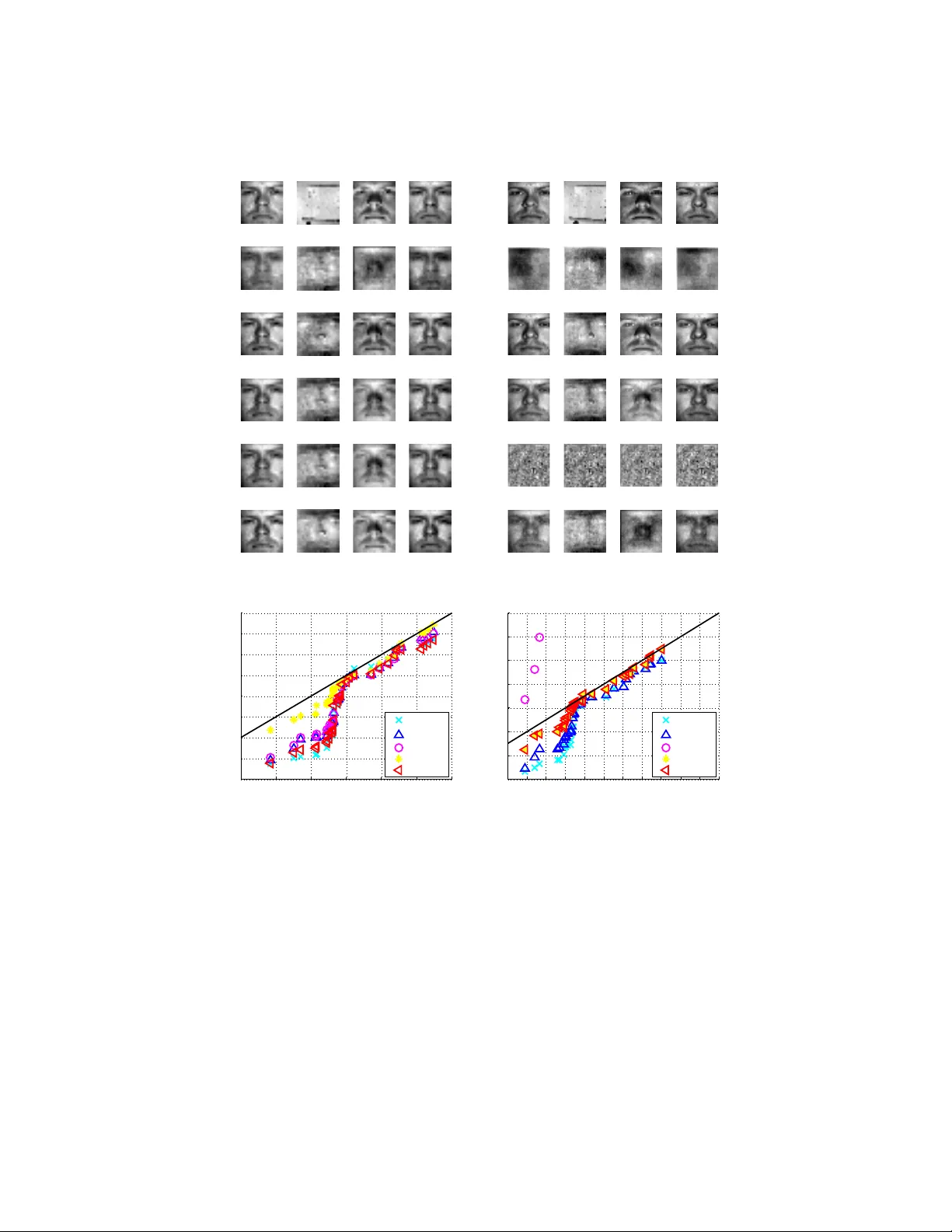
F ast, Robust and Non-con v ex Subspace Reco v ery G. Lerman , T. Maun u Scho ol of Mathematics, University of Minnesota Abstract This w ork presents a fast and non-con vex algorithm for robust subspace recov- ery . The data sets considered include inliers dra wn around a low-dimensional subspace of a higher dimensional am bient space, and a p ossibly large p ortion of outliers that do not lie nearb y this subspace. The proposed algorithm, which w e refer to as F ast Median Subspace (FMS), is designed to robustly determine the underlying subspace of suc h data sets, while having low er computational com- plexit y than existing metho ds. W e prov e conv ergence of the FMS iterates to a stationary p oin t. F urther, under a sp ecial mo del of data, FMS conv erges to a p oin t whic h is near to the global minimum with ov erwhelming probability . Un- der this mo del, we sho w that the iteration complexity is globally b ounded and lo cally r -linear. The latter theorem holds for any ﬁxed fraction of outliers (less than 1) and an y ﬁxed p ositiv e distance b et w een the limit p oin t and the global minim um. Numerical exp erimen ts on syn thetic and real data demonstrate its comp etitiv e sp eed and accuracy . 1. In tro duction In the mo dern age, data is collected in increasingly higher dimensions and massiv e quan tities. An imp ortan t metho d for analyzing large, high-dimensional data inv olves modeling it by a lo w-dimensional subspace. By pro jecting the data on this subspace, one can signiﬁcantly reduce the dimension of the data while capturing its most signiﬁcan t information. Classically , this is the problem of principal comp onen t analysis (PCA), which ﬁnds the subspace of maximum v ariance. PCA is eﬃciently implemen ted for moderate-size data b y using the singular v alue decomposition (SVD) of the data matrix. F or larger data, recen tly dev elop ed random SVD metho ds ha ve b een prov ed to b e stable, accurate and fast [21]. Despite the impressive progress with eﬀective algorithms for PCA, the un- derlying idea of PCA is completely useless when the data is corrupted. Among the many p ossible mo dels for corrupted data sets, here w e follow an “inliers- outliers” corruption mo del. More precisely , w e assume that some of the data p oin ts (the inliers) are sampled around a d -dimensional subspace, whereas, the rest of them (the outliers) are sampled from a diﬀeren t (and p ossibly arbitrary) Pr eprint submitte d to Elsevier mo del. The problem of Robust Subspace Reco very (RSR) asks to robustly es- timate the underlying low-dimensional subspace in the prese nce of outliers. W e note that this problem is distinct from what is commonly referred to as “ro- bust PCA”, that is, recov ering the low rank structure in a matrix with sparse elemen t-wise corruptions (see e.g., the work of Cand` es et al. [10]). Experience has dictated that robust PCA algorithms tend to p erform p oorly in the RSR regime, esp ecially when the proportion of outliers is high. Much recen t w ork has b een dev oted for developing numerically eﬃcien t solutions of the RSR problem. Curren t batch RSR formulations are at best comparable to full PCA (which computes all D eigenv ectors). That is, their complexit y is of order O ( T N D 2 ), where T is the n umber of iterations till conv ergence, N is the num b er of p oin ts and D is the ambien t dimension. W e are una ware of suﬃciently accurate RSR batc h algorithms that scale at least like O ( T N D d ), where d is the dimension of the appro ximated subspace. T o address this void, we prop ose a nov el non-con vex algorithm for RSR: the F ast Median Subspace (FMS) algorithm. The computational cost of FMS is of order O ( T N Dd ), which not only dep ends linearly on D (when d is small), but empirically FMS seems to obtain the smallest T and the highest accuracy among all other RSR algorithms (the T yler M-estimator [57, 65] has comparable accuracy in many cases, but its computational cost p er iteration is signiﬁcantly larger with mo derate or high ambien t dimensions). Theoretical guarantees un- der a mo del of corrupted data and empirical tests demonstrate the merit of the FMS algorithm. 1.1. Pr evious Works PCA is b y no w a classic and ubiquitous metho d in data analysis [29]. Since it is obtained by the SVD of the data matrix, it enjoys a w ealth of eﬃcient n umer- ical metho ds. In the last decade, v arious random metho ds hav e b een prop osed for fast and accurate computation of the top singular vectors and v alues (see the review by Halko et al. [21]). F or example, Lib ert y et al. [38] demonstrated an order of O ( N D log( d ) + ( N + D ) d 2 ) randomized algorithm for d -approximation PCA; and Rokhlin et al. [51] hav e com bined random dimension reduction with the pow er method to obtain a PCA algorithm with C N D d complexity (where C is a small constant) and with signiﬁcantly impro ved accuracy when the singular v alues decay suﬃcien tly fast. The complexity of state-of-the-art algorithms for online PCA [4, 5] is at b est of order O ( T D d ); how ever, in practice T is often large and their accuracy is often not comp etitiv e. While PCA is ubiquitous for subspace mo deling without corruption, there is still not yet a clear choice for a b est RSR algorithm. Many strategies for RSR hav e b een established in the last three decades (see the review by Lerman et al. [34] and some of the recent developmen ts by Xu et al. [60, 61], McCoy and T ropp [46], Zhang and Lerman [66], Lerman et al. [34], Zhang [65], F eng et al. [19], Hardt and Moitra [23], and Go es et al. [20]). Most of the emphasis of the theoretical analysis of RSR algorithms has b een on quantifying the largest p ercen tage of outliers under which the studied algorithm can be suﬃcien tly accurate [61, 34, 66, 65, 23]. In particular, Hardt and Moitra [23] hav e shown 2 that guaran teeing the success of an RSR algorithm with a fraction of outliers larger than ( D − d ) /D for a broad range of instances is as hard as solving the small set expansion problem; they also show ed that this fraction can b e ac hieved in their setting; though it is p ossible to achiev e a b etter fraction in sp ecial instances [66, p. 766]. As opp osed to the algorithms of Lerman et al. [34], Zhang and Lerman [66], Zhang [65], and Hardt and Moitra [23], other RSR algorithms ma y not b e accurate with high p ercen tage of outliers. T able 1 in [66] summarizes theoretical b ounds for the p ercen tage of inliers to outliers required for recov ery . All of the algorithms in this table asymptotically dep end on d and D , where some also dep end on the v ariances of inliers and outliers. Man y of the successful RSR algorithms inv olve minimizing an energy , which is robust to outliers. F or example, Xu et al. [61, 60], McCoy and T ropp [46], Zhang a n d Lerman [66], Lerman et al. [34], and Goes et al. [20] use conv ex relaxations of the same energy , which is later formulated in (1) when p = 1 and δ = 0. W e b eliev e that since FMS targets the original robust energy and not a conv ex relaxation of it, FMS achiev es higher accuracy and p ossibly even faster con vergence; how ev er, its analysis is diﬃcult due to the non-con vexit y . The Tyler M-estimator minimizes a p ossibly more robust energy and thus ob- tains competitive accuracy (empirically , our metho d is as accurate as T yler’s M-estimator). How ever, it cannot obtain suﬃciently comp etitiv e sp eed since it requires full eigen v alue decomp osition as well as initial dimensionalit y reduc- tion by PCA on to a subspace whose dimension is of the order of the num ber of p oin ts. While many of these algorithms for RSR are not suﬃciently fast, others are also not very well justiﬁed in theory . F or example, HR-PCA [60] and DHR- PCA [19] quan tify their recov ery by the ”expressed v ariance” (EV), but their actual b ounds seem to b e weak. This is evident in Theorem 2 of [19], whic h giv es asymptotic guarantees. Consider the case of 10% outliers drawn from a standard Gaussian, and inliers drawn from a standard Gaussian restricted to a subspace. Then it can b e sho wn that their low er b ound for EV is 0.09; an EV of 1 amoun ts to exact recov ery . On the other hand, the pro cedures of Hardt and Moitra [23] do not inv olve robust energy minimization, but try to ﬁt many diﬀerent subspaces until suc- cess. They are not suﬃciently fast and w e are unfamiliar with truly c ompetitive implemen tations of them. Online algorithms [67, 20] for RSR suﬀer from the same problems of online PCA algorithms men tioned ab o v e. Namely , the num- b er of iterations required can b e quite large, and their accuracy is often not comp etitiv e. An imp ortan t algorithm to compare with is spherical PCA (SPCA). SPCA in volv es p erforming PCA on the data after it is centered and then pro jected to the unit sphere. Maronna et al. [45] determined that SPCA was their metho d of choice when compared with v arious RSR algorithms [44]. F urther, the com- plexit y of running SPCA on a data set is O ( N D d ), whic h is faster than FMS by a m ultiplicative constant. Our tes ts indicate that while SPCA is faster, it do es not ac hieve the comp etitiv e accuracy of FMS on subspace recov ery problems in the numerical tests of § 4. Similarly to SPCA, many energy-minimization based algorithms (in particular, [61, 46, 66, 34, 20]) b eneﬁt from initial data 3 normalization to the unit sphere (after robust centering). Indeed, while their underlying energies are robust to high p ercen tages of some outliers, they ma y b e sensitive to adversary outliers of very large magnitude. It is also worth noting a couple recent works which scale to larger data than previous RSR algorithms. The w ork on Adaptiv e Compressiv e Outlier Sampling b y Li and Haupt [37], can be view ed as a solution to the RSR problem with drastically reduced complexity that dep ends on how man y rows and columns of the data are selected. Ho wev er, it is not as eﬀective at precisely identifying the underlying subspace as our metho d, which stems from the fact that it builds on Outlier Pursuit (OP) [61] (i.e. it is an approximate version of OP , which is not accurate enough). OP could not comp ete with the accuracy of other RSR algorithms in many of the regimes w e test. Another recent algorithm with the p oten tial to scale as w ell as FMS for RSR is the work on Grassmann Aver- ages [24], pro vided that the correct robust function µ rob is chosen. How ev er, Grassmann Averages lack any sort of theoretical justiﬁcation, b oth for conv er- gence and robustness. A similar algorithm to FMS is explored in W ang et al. [59], which prop osed a non-conv ex robust PCA algorithm. Although their algorithm is not suited for the RSR problem, it was still relev an t for our work on FMS. First, we borrow ed from W ang et al. [59] an argument for the proof of con vergence of the FMS iterates to a stationary p oin t (it is one of several diﬀeren t argumen ts used in our proof ). Second of all, the FMS algorithm migh t be view ed as a soft analog of the alternating least squares (ALS) pro cedure of [59] (FMS divides by a p o w er of the distance to a subspace and ALS divides b y 1 or “inﬁnit y”; FMS applies randomized SVD, whereas ALS applies alternating lo w-rank approximation). Finally , there are many recen t w orks on the analysis of non-conv ex algo- rithms and their surprising eﬀectiveness on problems with structured data. Some examples include w orks b y Sun et al. [53, 54], Zhang and Balzano [64], Jain et al. [28], Dauphin et al. [16], Kesha v an et al. [31, 32], Boumal [8], and Bandeira et al. [6]. In particular, there has b een related work on non-conv ex analysis re- lated to low rank mo deling (see the work of Keshav an et al. [31, 32], Jain et al. [27], Hardt [22], Netrapalli et al. [48], Jain and Netrapalli [26], Jain et al. [28], and Zhang and Balzano [64] for some examples). Our analysis of FMS presents y et another example where a non-conv ex algorithm is surprisingly accurate in lo w rank mo deling despite p oten tial issues of non-conv ex optimization, such as slo w con vergence or conv ergence to a non-optimal point. W e also p oin t the reader to the work of Daub ec hies et al. [15], which aims at analyzing the con- v ergence of an IRLS method when the energy is non-con vex. Although their metho d is for a diﬀeren t problem, there is a strong similarity in the use of non-con vex energies: in their case when τ < 1 and in our case when p < 1. 1.2. This Work The FMS algorithm impro ves on existing metho ds due to its fast runtime and state-of-the-art accuracy . Ho w ever, the underlying minimization of FMS is non-con vex and thus diﬃcult to analyze. This work contributes to non-conv ex 4 analysis and direct optimization on the Grassmannian manifold G ( D , d ) in the follo wing wa ys: 1. W e prov e con vergence of the FMS iterates to a stationary p oin t o ver G ( D , d ). 2. F or t wo sp ecial mo dels of data, w e prov e: • This stationary point is suﬃcien tly close to the global minimum with o verwhelming probability; • The con vergence rate is globally b ounded and lo cally r -linear. These t wo mo dels are: (a) Inliers are dra wn from a spherically symmetric distribution restricted to a ﬁxed subspace L ∗ 1 and outliers are dra wn from a spherically symmetric distribution in the whole space; (b) The subspace dimension is d = 1 and outliers are either symmetrically distributed in the ambien t space or lie on another subspace L ∗ 2 (where it is less probable to dra w p oin ts from L ∗ 2 than L ∗ 1 ). 3. F or b oth models in 2, w e guarantee appro ximate recov ery for any percent- age of outliers (less than 1); the theory of other RSR algorithms requires b ounds on this p ercen tage. 4. Out of all other RSR algorithms, we pro vide the only guarantees for the mo del 2b. In addition to the theory , we rely on careful numerical exp erimen tation and b eliev e that the results rep orted in this paper strongly indicate the merit of FMS. The FMS algorithm displa ys comp etitiv e speed and accuracy on synthetic data sets. Unlike other RSR algorithms, FMS also shows strong performance as a dimension reduction to ol for clustering data since it scales well, as we demonstrate on the h uman activity recognition data in § 4.2.2. 1.3. Structur e of The Pap er This paper b egins b y motiv ating and outlining our new algorithm in § 2. Next, § 3 establishes conv ergence of the FMS iterates to a stationary p oin t, and further gives optimality and rate guarantees for FMS under a certain mo del of data. Exp erimen ts on synthetic and real data (of astrophysics, h uman activity , and face recognition) are done in § 4 to demonstrate the usefulness of our new approac h. Lastly , § 6 concludes this work. 2. The FMS Algorithm This section presents the FMS algorithm. First, § 2.1 presen ts basic notation used throughout the pap er. Then, in § 2.2 w e describ e its underlying minimiza- tion problem and its robustness. Next, in § 2.3 we prop ose the FMS algorithm, while motiv ating it in a heuristic wa y . Finally , § 2.4 summarizes its complexity , and § 2.5 discusses the c hoices of parameters for the FMS algorithm. 5 2.1. Notation W e assume a data set of N p oin ts in R D , X = { x i } N i =1 . W e seek an appro ximating d -dimensional subspace, L , or in short a d -subspace. W e de- note by G ( D , d ) the Grassmannian manifold of linear d -subspaces of R D . F or L ∈ G ( D , d ) we denote by P L the orthogonal pro jector onto L , which we view as an elemen t of R D × D . Let k · k denote the Euclidean norm on R D . F or x ∈ R D and L ∈ G ( D , d ) we denote b y dist( x , L ) the Euclidean distance of x to L , that is, k x − P L x k . F or the distance b et w een L 1 , L 2 ∈ G ( D , d ), which we denote b y dist( L 1 , L 2 ), we use here the square-ro ot of the sum of the squared principal angles b et w een L 1 and L 2 . 2.2. The Underlying Minimization Pr oblem Man y approac hes for RSR are motiv ated b y the follo wing minimization prob- lem: F or the data set X ⊂ R D , 0 0, ﬁnd a d -subspace L that minimizes among all suc h subspaces the energy F p,δ ( L ; X ) = X 1 ≤ i ≤ N dist 2 − p ( x i ,L ) ≥ pδ dist p ( x i , L ) + X 1 ≤ i ≤ N dist 2 − p ( x i ,L ) 0 and mo dify the w eight to b e 1 / max(dist( x i , L k ) 2 − p , pδ ) (an explanation for this regularized term follo ws from (29) whic h app ears later in the pro of of Theorem 1). T o solve the w eighted PCA problem, one ﬁrst needs to weigh t the cen tered data p oin ts b y the latter term and then apply PCA (without centering) to compute L k +1 . The abilit y to directly apply PCA, or equiv alen tly SVD, to the scaled data matrix is numerically attractive, and we can apply any of the state-of-the-art suites for it. Our procedure at iteration k is outlined as follows. First, form the new w eighted data p oin ts y i = x i / max(dist( x i , L k ) (2 − p ) / 2 , p pδ ) , 1 ≤ i ≤ N . (4) Then, compute top d righ t singular vectors of the data matrix Y , whose columns are the weigh ted data p oin ts { y i } N i =1 (for SVD, we found the randomized metho d 7 of Rokhlin et al. [51] to b e suﬃciently fast without sacriﬁcing accuracy). The subspace L k +1 is then the span of these vectors. This pro cedure is iterated un til L k suﬃcien tly con v erges. W e formally call this iterative pro cedure the F ast Median Subspace (FMS) and summarize it in Algorithm 1 (for simplicity w e use the notation  for √ pδ used ab o ve). Algorithm 1 F ast Median Subspace (FMS p ) 1: Input: X = [ x 1 , . . . , x N ]: D × N cen tered data matrix, d : desired rank, p : robustness p o wer (0 < p < 2; default: p = 1), n m : maxim um n umber of iterations, τ ,  : parameters (default: 10 − 10 for b oth) 2: Output: L : d -subspace in R D 3: k ← 1 4: L 0 ≡ L 1 ← PCA d -subspace in R D 5: while k < n m and dist( L k , L k − 1 ) > τ do 6: for i=1:N do 7: y i ← x i / max(dist( x i , L k ) (2 − p ) / 2 ,  ) 8: end for 9: Y ← [ y 1 , . . . , y N ] 10: [ U , S , V ] ← RandomizedPCA( Y , d ) [51]; 11: L k +1 ← column space of U 12: k ← k + 1 13: end while In practice, w e hav e found that the rate of con vergence of the FMS algo- rithm is not aﬀected b y its particular use of RandomizedPCA [51]. In other w ords, if RandomizedPCA is replaced with the exact SVD, the conv ergence and accuracy are the same, but RandomizedPCA results in shorter runtime. Also, it seems adv an tageous to initialize L 0 with the result of RandomizedPCA (or SVD) on the full data set X , although initialization can also b e done randomly . Random initialization is not recommended, though. F or example, in a regime where outliers lie on another weak er subspace, starting to o close to the outlier subspace can result in conv ergence to a lo cal minimum rather than the global minim um. Empirically , with PCA initialization in these cases, FMS conv erges to the stronger subspace (i.e. it conv erges to the global minimum). Finally , we denote the FMS algorithm run with a parameter p by FMS p for the remainder of the pap er. 2.4. Complexity A t eac h iteration, FMS p creates a scaled data matrix of cen tered data p oin ts, whic h takes O ( DN d ) op erations, although the scaling can b e done in parallel. It then ﬁnds the top d singular vectors of the scaled data matrix to up date the subspace, whic h tak es O ( D N d ). Th us, the total complexit y is O ( T DN d ), where T is the num b er of iterations. Empirically , w e ha ve noticed that T can be treated as a relativ ely small constant. F or example, in the sp ecial case of Theorem 5, T ≤ O  1 / ( pδ min(1 , η 3( p − 1) ))  for an η -approximation to the limiting stationary 8 p oin t. This further reduces to T = O (log(1 /η )) if the iterates are suﬃciently close to the limiting stationary p oin t by Theorem 6. The storage of the FMS p algorithm in volv es the N × D data matrix X and the weigh ted data matrix Y at eac h iteration. FMS p m ust also store the D × d bases for the subspaces L k and L k +1 . Thus, the storage requirement for FMS p is 2 D N + 2 D d . 2.5. Choic e of Par ameters p , δ , and d In the later experimental sections (see § 4), w e compare FMS p run with p = 1 and p = 0 . 1. Although there is not alwa ys a diﬀerence, in some cases w e see one of the tw o c hoices of p p erforming b etter than the other. There also does not app ear to b e an adv an tage for using 1 < p < 2. Curren tly , the theory seems to supp ort p = 1 for the b est rates of recov ery (see Theorem 2). F urther, the theory seems to also indicate that smaller p leads to less robustness to higher lev els of noise (see Theorem 3). Later experiments in § 4 indicate that with small num b ers of p oin ts, a choice of small p < 1 can lead to conv ergence to a non-optimal p oin t, while p = 1 is still able to conv erge (see Figures 9 and 10). W e b eliev e that p can b e optimized for a sp eciﬁc data set, given some prior kno wledge of it. In other w ords, p can be chosen if the user designates a training data set where the truth is kno wn. Due to the low complexit y of the method, it is p ossible to eﬃciently run it ov er an array of v alues of p . Thus, with the sp eciﬁed training set, cross-v alidation can b e used to select the prop er v alue of p for a giv en type of data, although this requires the user to ha ve some prior kno wledge of the data. F or choice of δ , we hav e not noticed to o muc h diﬀerence b et w een diﬀeren t v alues, although there may b e certain cases where it is necessary to b e careful with the choice of δ . In Theorem 2, we see rates of asymptotic recov ery for the FMS p algorithm under a sp ecial mo del of data. This theory seems to p oin t to taking δ as small as p ossible when 1 ≤ p < 2, but to take larger v alues of δ when 0 < p < 1. F urther, some exp erimen ts with smaller sample sizes indicate that using a parameter δ to o small with p < 1 can lead to con vergence to a non-optimal p oin t (i.e. a lo cal minimum). Thus, while we advocate choosing δ as small as p ossible, some care must b e taken when p < 1 to ensure that δ is not c hosen to b e to o small. Finally , one may ask ho w to select the subspace dimension d for FMS p . Pic king the correct subspace dimension d is not well studied or justiﬁed in the literature. Heuristic strategies, suc h as the elb o w metho d, can b e used to guess what the b est subspace dimension is; such strategies usually require a test o ver a range of p ossible v alues for d . On the other hand, in some domains there is prior knowledge of d . F or example, in facial recognition type datasets, images of a p erson’s face with constan t p ose under diﬀering illumination conditions appro ximately lie on a d = 9 dimensional subspace [7]. In practice, we advocate either using the elb o w metho d or domain kno wledge to select the b est v alue for d . 9 3. Theoretical Justiﬁcation Since FMS p prop oses an iterative pro cess it is rather imp ortan t to analyze its con vergence. In § 3.1, w e form ulate the main conv ergence theorem, whic h establishes conv ergence of FMS p to a stationary p oin t (or contin uum of station- ary p oin ts). Next, § 3.2 assumes the data is sampled from a certain distribution and pro ves that FMS p con verges to a p oin t near to the global minimum with o verwhelming probability . In § 3.3, it is further shown under this mo del that the rate of con vergence is globally bounded and lo cally r -linear (again with o verwhelming probability). The pro ofs of all theorems are left to § 5. 3.1. Gener al Conver genc e The or em W e establish con vergence to a stationary point of the energy F p,δ o ver G ( D , d ): Theorem 1 (Conv ergence to a Stationary P oint). L et ( L k ) k ∈ N , b e the se- quenc e obtaine d by applying FMS p without stopping for the data set X for a ﬁxe d 0 < p < 2 . Then, ( L k ) k ∈ N c onver ges to a stationary p oint L ∗ of F p,δ over G ( D , d ) , or the ac cumulation p oints of ( L k ) k ∈ N form a c ontinuum of stationary p oints. The pro of the theorem appears in § 5.1. While there are no assumptions on X , it is imp ortan t to discuss the implications of this Theorem. In § 3.1.1 w e discuss the p ossibilit y that FMS p con verges to a con tinuum of stationary p oin ts. Then, § 3.1.2 discusses the p ossibilit y of conv ergence to a saddle p oin t, and § 3.1.3 discusses con vergence to a lo cal minimum. 3.1.1. Conver genc e to a Continuum of Stationary Points Theorem 1 prov es conv ergence of the FMS p iterates to a stationary p oin t or a contin uum of stationary p oin ts. Another wa y to think of this issue is that the contin uum of stationary p oin ts is also a contin uum of ﬁxed p oin ts for the FMS p algorithm. It is desirable to know when the algorithm conv erges to a single p oin t v ersus a con tinuum. Ho wev er, while we cannot see how to rule out the contin uum case, w e also cannot construct an example of a discrete data set with a c on tin uum of stationary p oin ts when the rank of the data set is less than the subspace dimension d . When the rank of the data is less than d , all subspaces con taining the data set are essentially equiv alen t with resp ect to the data. W e conjecture that w e ha ve actual con vergence to a single stationary p oin t of G ( D , d ) for data sets which are full rank. 3.1.2. Can ( L k ) k ∈ N Conver ge to a Sadd le Point? While we prov e conv ergence to a stationary p oin t of F p,δ o ver G ( D , d ), we are not able to say what kind of a stationary p oin t w e conv erge to. In theory we cannot rule out a saddle p oin t, but w e are unaw are of an example of a saddle p oin t which is also a ﬁxed p oin t of FMS p . The following example describ es a 10 saddle p oin t of F p,δ whic h is not a ﬁxed p oin t of FMS p with probabilit y 1. F or this example, w e assume that if the solution to PCA is not unique, then the PCA output is selected uniformly at random from the solution set. Consider the data set in R 3 X =  (1 , 0 , 0) T , (0 , 1 , 0) T  . (5) F or the FMS p energy function F p,δ , the line deﬁned by ` sad = Sp([1 , 1 , 0] T ) is a saddle p oin t for the FMS p energy , since it is a minim um along the geo desic from ` max = Sp([0 , 0 , 1] T ) to ` sad , but a maximum along the geo desic from ` min 1 = Sp([1 , 0 , 0] T ) to ` min 2 = Sp([0 , 1 , 0] T ). How ev er, ` sad is not a ﬁxed p oin t of FMS p . Suppose that ` sad is selected as a candidate subspace b y FMS p . Then, the tw o data p oin ts x and x 2 are equidistant from ` sad and are scaled by the same amount. Then, when PCA is done to ﬁnd the new subspace from the scaled data, all lines along the geo desic from ` min 1 to ` min 2 are solutions, and th us ` sad is selected again with probabilit y 0. After a new line is selected, the p oin ts will no longer b e equidistant and one of the tw o p oin ts will dominate the next round of PCA. This giv es conv ergence to either ` min 1 or ` min 2 . W e also see examples of asymptotic saddle points in the mo del considered in § 3.2. How ever, it can b e sho wn with ov erwhelming probability that the ﬁnite sample counterparts to these asymptotic saddle p oin ts are not ﬁxed p oin ts. Th us, in general, we are not concerned with saddle points that are also ﬁxed p oin ts, since we hav e no pro of that such a p oin t exists. 3.1.3. Conver genc e to L o c al Minima Unlik e PCA (i.e. when p = 2), there can p oten tially b e many lo cal minima for the energy F p,δ when 0 < p < 2 . Such lo cal minima can also b e ﬁxed p oin ts for the FMS p algorithm. Hence, we cannot guarantee that FMS p con verges to an optimal stationary p oin t in general, since it could con verge to one such lo cal minima. F or example, some lo cal minima are discussed b y Lerman and Zhang [36, Example 2] when δ = 0. A mo diﬁed argument can b e used to show that lo cal minima still exist when δ > 0. W e observe that local minima generally o ccur when p oin ts concen trate around low er dimensional subspaces. Another simple example with many lo cal minima is a symmetric case when D = 2 and d = 1. Supp ose that p oin ts are symmetrically distributed on S 1 : for some ev en N ∈ N , the data set consists of p oin ts x i = (cos(2 π i/ N ) , sin(2 π i/ N )) T , i = 1 , . . . , N . Then, the span of each pair of antipo dal p oin ts will deﬁne a lo cal minim um for the FMS p energy F p,δ . Ho wev er, we note that in this case all lo cal minima are also global minima. 3.2. Conver genc e to the Glob al Minimum for a Sp e cial Mo del of Data In this section, w e will show that under a certain mo del of probabilistic gen- eration of the data, the FMS p algorithm nearly recov ers an underlying subspace with ov erwhelming probability (w.o.p.). By w.o.p., we mean that the probabilit y of recov ery is b ounded b elow by an expression of the form 1 − C 1 e − C 2 N , where C 1 and C 2 are constan ts with respect to N (but dep end on all other parameters, 11 suc h as d , D , p , and δ ). In § 3.2.1 w e lay out some necessary concepts for the statemen t of the theorems, and then in § 3.2.2 we state the theorem giving near reco very of the underlying subspace. Next, § 3.2.3 extends to a sp ecial case of reco very with multiple subspaces. 3.2.1. Pr eliminaries This section prov es global conv ergence for a sp ecial mo del of data. W e use a simple v ersion of the most signiﬁcan t subspace mo del outlined in [36], and m uch of the notation and concepts are b orro w ed from this pap er. The general setting considers p oin ts distributed on the sphere S D − 1 . In § 3.2.2 we consider the sp ecial case of one underlying subspace , rather than the more general setting of K distinct underlying subspaces with one most signiﬁcant. A more general theorem for K > 1 has b een hard to prov e, although § 3.2.3 gives a theorem for appro ximate reco very in the case K = 2 and d = 1. Ho wev er, w e conjecture that a general theorem for K > 1 holds with any subspace dimension d due to empirical p erformance of the algorithm on data sets sampled from these distributions. Let L ∗ 1 b e the most signiﬁcant subspace within our data set. W e construct a mixture measure by combining µ i for i = 0 , ..., K , where µ 0 is the uniform distribution on S D − 1 and µ i is the uniform distribution on S D − 1 ∩ L ∗ i . In the noisy case, we add an additiv e noise distribution ν i,ε suc h that supp( µ i + ν i,ε ) ⊆ S D − 1 . W e also require that the p th momen t of ν i,ε is smaller than ε p (where p is the robustness parameter for FMS). Finally , we attac h weigh ts α 0 ≥ 0 , α i > 0 to the measures µ i suc h that P K i =0 α i = 1 and α 1 > P K i =2 α i . The mixture distribution is giv en by µ ε = α 0 µ 0 + K X i =1 α i ( µ i + ν i,ε ) . (6) W e ﬁrst consider a noiseless v ersion of µ ε , and then extend the result to the noisy case. The noiseless measure is written as µ = α 0 µ 0 + K X i =1 α i µ i . (7) W e assume data sampled indep enden tly and identically from µ , so that p oin ts sampled from µ 0 and µ i for i = 2 , ..., K represent pure outliers, and p oin ts sampled from µ 1 represen t pure inliers. Ev erything we prov e for the spherical mo del we can generalize to a spherically symmetric model, where outliers are spherically symmetric and symmetrically distributed on K − 1 less signiﬁcant subspaces, and inliers are symmetrically distributed on the most signiﬁcant subspace L ∗ 1 . Note that in practice, normalizing the latter distribution to the sphere S D − 1 yields a mixture measure of the form (7). 12 3.2.2. Glob al Conver genc e The or em for K = 1 W e are no w ready to state a global conv ergence theorem for FMS p . Theorem 2 (Probabilistic Recov ery of the Underlying Subspace). L et X b e sample d indep endently and identic al ly fr om the mixtur e me asur e µ given in (7) with K = 1 . Then, for any 0 < η ≤ π / 6 and 0 < p ≤ 1 , the FMS p al- gorithm c onver ges to an η -neighb orho o d of the underlying subsp ac e L ∗ 1 w.o.p. at le ast 1 − C 1 e − C 2 N ( pδ ) 2(1 − p ) / (2 − p ) min  ( π 6 ) 2( p − 1) , η 2 ( pδ ) 2  . (8) F or 1 < p < 2 , the FMS p algorithm c onver ges to an η -neighb orho o d of the underlying subsp ac e L ∗ 1 w.o.p. at le ast 1 − C 0 1 e − C 0 2 N min  η 2( p − 1) , η 2 ( pδ ) 2  . (9) F or c omp arison, using the same te chniques to analyze PCA ( p = 2 ), PCA out- puts a subsp ac e in an η -neighb orho o d of L ∗ 1 w.o.p. at le ast 1 − C 00 1 e − C 00 2 N η 2 . (10) Her e, C 2 , C 0 2 , and C 00 2 have no dep endenc e on N , η , p , or δ , but may dep end on D and d . The pro of of this theorem is giv en in § 5.2. This theorem gives a probabilis- tic near reco very result for the FMS p algorithm and PCA. W e note that the result given for PCA is comparable to the asymptotic result of V ershynin [58, Prop osition 2.1], alb eit by a diﬀerent argument. Our result is more restricted, though, since the result of V ershynin [58, Prop osition 2.1] applies for any η > 0. Also, our estimates for the PCA constants (see b elo w) are not ideal (again see [58]); how ev er, this is not an issue since we are more in terested in contrasting the dep endence of these probabilities on η . There is no restriction on α 0 and α 1 in (7), although the probability of recov ery dep ends on the fractions. Bounds for the constants C 2 , C 0 2 and C 00 2 can b e seen later in (79), (80), and (81) resp ec- tiv ely . W orst case estimates of C 1 , C 0 1 and C 00 1 are given later in Prop osition 4, where w e examine their dep endence on d , D , η , p , and δ . This theorem shows the b eneﬁt of using FMS p o ver PCA. F or the following discussion, w e follo w our default choice of the algorithm and assume that δ is on the order of mac hine precision. This means that we only need to consider the ﬁrst term within the minimum function in (8) (since η cannot b e low er than mac hine precision). Examining dependence on η for the probabilit y b ounds, the exp onen t in the PCA formulation is O ( η 2 N ), the FMS 1 exp onen t is O ( N ), and for p < 1 the FMS p exp onen t is O (( pδ ) 2(1 − p ) / (2 − p ) N ). Altogether, this means that FMS p is exp ected to hav e muc h more precise recov ery for v astly smaller sample sizes. W e also advocate choosing p = 1 when running the FMS p algorithm for this reason: when δ is c hosen to b e very small in this w ay , the O (( pδ ) 2(1 − p ) / (2 − p ) N ) exp onen t for p < 1 leads to a muc h worse b ound than 13 the O ( N ) exp onen t for p = 1. Another consequence of this theorem is that w e generally advocate for larger v alues of δ for smaller v alues of p (although we do not hav e optimal expressions for this choice of δ ). F or demonstrations of the phase transitions exhibited b y the probabilit y of reco very , see Figures 5, 6, and 7. Again, we emphasize the diﬀerence b et ween the b ounds on the probabilities of η -reco v ery for PCA, FMS 1 , and FMS 0 . 5 : their b ounds are 1 − C 00 1 e − C 00 2 η 2 N , 1 − C 1 e − C 2 O (1) N , and 1 − C 1 e − C 2 O ( δ 2 / 3 ) N resp ectiv ely . The theoretical result of Theorem 2 extends to the noisy mixture measure (6) as w ell. Theorem 3. L et X b e sample d indep endently and identic al ly fr om the noisy mixtur e me asur e µ ε given in (6) . Then for any 0 < η ≤ π / 6 , if 0 < p ≤ 1 and ε <  1 4 2 π d 5 / 2 min   π 6  p − 1 η , η 2 pδ  1 /p , (11) the FMS p algorithm c onver ges to an η -neighb orho o d of L ∗ 1 w.o.p. state d in (8) . If 1 < p < 2 and ε <  1 4 2 π d 5 / 2 min  η p , η 2 pδ  1 /p , (12) the FMS p algorithm c onver ges to an η -neighb orho o d of L ∗ 1 w.o.p. state d in (9) . F or c omp arison, using the same te chniques to analyze PCA, if ε <  1 4 2 π d 2 η 2  1 / 2 , (13) PCA outputs a subsp ac e in an η -neighb orho o d of L ∗ 1 w.o.p. state d in (10) . The pro of of Theorem 3 is given in § 5.2.4. Among choices of p , choosing larger v alues of p seems to give the most robustness to noise. This theorem indicates that PCA has the b est stabilit y to noise, although these estimates are not ideal. This result stands in contrast to the result of [13], which sho ws a higher robust- ness to noise for a conv ex relaxation of F 1 ,δ . Less robustness to noise for FMS p ma y b e attributable to non-conv exit y , but we cannot make any deﬁnitive state- men t on this fact. In the future, we plan to follow Coudron and Lerman [13] and establish the stronger robustness to noise of FMS p at least when p = 1. F or demonstrations of the phase transitions exhibited by the probabilit y of reco very for this noisy mo del, see Figures 8, 9, and 10. 3.2.3. Glob al Conver genc e The or em for K = 2 and d = 1 Another imp ortan t setting of the most signiﬁcan t subspace model where PCA do es not recov er the underlying subspace is when K > 1. W e hav e found it hard to prov e anything in general for the case K > 1 b ecause it is hard to c haracterize the deriv ativ e of F p,δ in general. How ev er, w e are able to pro ve near reco very for the case K = 2 and d = 1. 14 Theorem 4 (Probabilistic Recov ery for K = 2 and d = 1 ). L et X b e sam- ple d indep endently and identic al ly fr om the mixtur e me asur e µ in (7) with K = 2 and d = 1 . Then, for any 0 < η ≤ π / 6 and 0 < p ≤ 1 , the FMS p algorithm with PCA initialization c onver ges to a p oint in B ( L ∗ 1 , max( η, arcsin(( pδ ) 1 / (2 − p ) ))) w.o.p. The pro of of Theorem 4 is giv en in § 5.3. It has prov en too hard to derive b ounds or closed form expressions for the constan ts in the probability b ound, and so we do not present them here. F urther, a similar stability result as that in Theorem 3 holds for Theorem 4, how ev er we do not display it here. W e also note that this Theorem only holds for 0 < p ≤ 1. This case is particularly imp ortan t b ecause the guarantees of other algorithms, suc h as those of Hardt and Moitra [23] and Zhang and Lerman [66], break down in this setting. F urther, although it is very sp eciﬁc, it is an imp ortan t example for us b ecause FMS p is still able to reco ver the correct subspace in the presence of another p oten tial lo cal minimum L ∗ 2 . Finally , this is a clear example where PCA cannot recov er the most signiﬁcan t subspace asymptotically while FMS p can. 3.3. R ate of Conver genc e for FMS p Under (7) F or this section, we deﬁne L ∗ to be a stationary limit p oin t of the FMS p algorithm. W e b egin with a probabilistic global rate of conv ergence b ound for the FMS p algorithm under (7) when K = 1 or K = 2 and d = 1. Under these mo dels, Theorem 2 and Theorem 4 show that L ∗ is near to L ∗ 1 (the underlying subspace) w.o.p. The pro of of Theorem 5 is giv en in § 5.4. Theorem 5 (Probabilistic Global Con vergence Bound). Supp ose that X is sample d i.i.d. fr om the mixtur e me asur e µ in (7) with K = 1 . Then, for 0 < p ≤ 1 , the numb er of iter ations T such that dist( L T , L ∗ 1 ) < η is at worst T = O   1 min   π 6  2( p − 1) pδ, η 2 ( pδ )    ( w.o.p. ) . (14) In c ontr ast, for 1 < p < 2 , the numb er of iter ations is at worst T = O   1 min  η 2( p − 1) pδ, η 2 ( pδ )    ( w.o.p. ) . (15) F or µ with K = 2 and d = 1 and 0 < p ≤ 1 , the numb er of iter ations T such that arcsin(( pδ ) 1 / (2 − p ) ) ≤ dist( L T , L ∗ 1 ) < η is at worst T = O  1 ( α 1 − α 2 ) 2 pδ  ( w.o.p. ) . (16) 15 Bey ond this, Theorem 6 yields local r -linear conv ergence w.o.p. for the FMS p algorithm under (7) when K = 1 or when K = 2 and d = 1. The proof of Theorem 6 is giv en in § 5.5. Theorem 6 (Probabilistic Lo cal Linear Conv ergence). Supp ose that X is sample d i.i.d. fr om the mixtur e me asur e µ in (7) with K = 1 (or K = 2 , d = 1 , α 1 > (2 − p ) α 2 , and dist( L ∗ 1 , L ∗ 2 ) > 2 arcsin( pδ 1 / (2 − p ) ) ). Then, w.o.p., ther e exists an index κ such that ( L k ) k>κ c onver ges r -line arly to its limit p oint L ∗ . The b ound on the rate of this r -linear conv ergence can b e seen in the pro of of Theorem 6: sp eciﬁcally see (160) and (164). Theorems 5 and 6 can be combined to give a b ound on the ov erall iteration complexity of FMS p . In general, giv en a choice of p ≤ 1, the num ber of iterations required to con verge is b ounded by O  1 / ( pδ min(1 , η 3( p − 1) ))  (or O  1 / ( pδ ( α 1 − α 2 ) 4 )  when K = 2 and d = 1). Ho wev er, once the iterates are suﬃciently close to the limit p oin t, the iteration complexit y b ecomes O (log(1 /η )). Figure 11 veriﬁes that on a data set sampled from (7) with K = 1, the conv ergence of FMS 1 and FMS 0 . 5 is r -linear. 4. Numerical Exp erimen ts In this section, we illustrate ho w the FMS p algorithm p erforms on v arious syn thetic and real data sets in a MA TLAB test en vironment (except for § 4.2.4, whic h w as run in Python). It was most interesting for us to test FMS p with the v alue of p = 1, in order to compare it with v arious conv ex relaxations of its energy in this case. FMS 1 denotes a case where the algorithm run with a v alue of p = 1. In certain cases, we hav e not noticed a diﬀerence in the p erformance b y choosing lo wer v alues of p and will mak e clear when this is the case. In places where we noted such a diﬀerence we rep ort them with p = 0 . 1 and let FMS 0 . 1 denote the case of p = 0 . 1. W e set the parameter  to b e 10 − 10 . The algorithms we compare with are the T yler M-estimator [65], Median K-ﬂats (MKF) [67], Reap er [34], R1-PCA [17], GMS [66], and Robust Online Mirror Descen t (R-MD) [20]. W e also tried a few other algorithms, in particular, HR-PCA and DHR-PCA [60, 19], LLD [46], and Outlier-Pursuit [61], but they w ere not as comp etitiv e; we th us do not rep ort their results. F or example, b oth HR-PCA and DHR-PCA were slow er and surprisingly worse than PCA in man y of our tests. Ev en though MKF and R-MD w ere not comp etitiv e either in man y cases, it was imp ortan t for us to compare with online algorithms. The comparison with R1-PCA was also important since its aims to directly minimize (1) when p = 1 and δ = 0. In addition, we compared with principal comp onen t pursuit (PCP) [10, 39], whic h aims to solv e the robust PCA problem. The co de chosen for this comparison w as the Accelerated Proximal Gradient with partial SVD [40] obtained from http://perception.csl.illinois.edu/ matrix- rank/sample_code.html , although similar results were giv en b y the ALM co des [39]. W e emphasize that Robust PCA metho ds are designed for the regime where there are sparse, element-wise corruptions of the data matrix, rather than the wholly corrupted data p oin ts, which we consider in this pap er. 16 W e hav e noticed that robust PCA algorithms based on this mo del exhibit quite p oor p erformance compared to algorithms tailored for RSR when data p oin ts are wholly corrupted. Exp erimen ts by [34] demonstrate the adv antage of scaling eac h cen tered data p oin t b y its norm, i.e., by “spherizing” eac h data p oin t (equiv alen tly , pro jecting on to the unit sphere). In cases where we examine the eﬀect of ”spherizing” the data, we denote an algorithm run on a spherized data set with the preﬁx S. F or example, as a baseline in man y of the experiments we compare with SPCA, p erformed by using the RandomizedPCA [51] algorithm to ﬁnd the top d singular vectors of the spherized data. In the same vein, we sometimes also compare with SFMS p , whic h is FMS p run on spherized data. Spherizing seems to reduce noise and pro duce a b etter subspace in some cases: w e will displa y results from SFMS p and SPCA when this is the case (but omit them when there is no diﬀerence). T yler M-estimator is used with regularization parameter  = 10 − 10 . Median K-Flats passes ov er the data man y times to ﬁnd a single subspace of dimension d , with a step size of 0.01 and maximum n umber of iterations 10000. The Reap er algorithm is run with the regularization parameter δ = 10 − 20 . R1-PCA uses stopping parameter 10 − 5 and is capp ed at 1000 iterations. R-MD passes ov er the data 10 times and uses step size 1 / √ k at iteration k . The PCP parameter w as set as λ = 1 / p max( D , N ). 4.1. Synthetic Exp eriments A series of synthetic tests are run to determine how the FMS p compares to other state-of-the-art algorithms. In all of these examples the data is sampled according to v ariants of the needle-haystac k mo del of [34]. More precisely , inliers are sampled from a Gaussian distribution within a random linear d -subspace in R D , and outliers are sampled from a Gaussian distribution within the ambien t space. Noise is also added to all p oin ts. In all of these exp erimen ts, the fraction of outliers is restricted by Hardt & Moitra’s upp er b ound for RSR, that is, ( D − d ) /D [23]. The ﬁrst exp erimen t demonstrates the eﬀect of the p ercen tage of outliers on the total runtime and error for subspace recov ery . Let Σ in denote the or- thogonal pro jector onto the randomly selected subspace, and let Σ out denote the iden tity transformation on R D . In this exp erimen t, inliers are drawn from the distribution N (0 , Σ in /d ) and outliers from the distribution N (0 , Σ out /D ). Scaling b y 1 /d and 1 /D resp ectiv ely ensures that both samples ha v e comparable magnitudes. Error is measured by calculating the distance b et ween the found and ground truth subspaces. The ambien t dimension is ﬁxed at D = 100, the subspace dimension is d = 5, and the total n umber of points is ﬁxed at N = 200. Ev ery data p oin t is also p erturb ed by added noise drawn from N (0 , 10 − 6 Σ out ). Figure 1 displays results for reco very error and total run time v ersus the p er- cen tage of outliers in a data set. A t each p ercen tage v alue, the experiment is rep eated on 20 randomly generated data sets and the results are then a veraged. W e note that the runtime of R-MD is to o large to b e display ed on the graph of 17 Outlier Percentage 0 0.1 0.2 0.3 0.4 0.5 0.6 0.7 0.8 0.9 1 log-Recovery Error -6 -5 -4 -3 -2 -1 0 1 2 (a) Outlier Percentage 0 0.1 0.2 0.3 0.4 0.5 0.6 0.7 0.8 0.9 1 Total Runtime (s) 0 0.2 0.4 0.6 0.8 1 1.2 1.4 1.6 1.8 2 FMS 0.1 FMS 1 Tyler Reaper SPCA R-MD R1-PCA MKF GMS PCP (b) Figure 1: Plots demonstrating the accuracy and total runtime of some subspace reco very algorithms versus the p ercen tage of outliers in the data set (b ounded b y the upp er b ound of [23] for RSR). FMS 1 and FMS 0 . 1 obtain b oth comp etitiv e time and accuracy , with the exception of FMS 1 for 95% outliers. total runtime. FMS 0 . 1 and Tyler M-estimator hav e the b est accuracy on this data, while FMS 1 only demonstrates problems at high ends of outlier p ercen t- ages. Out of the robust metho ds, FMS 1 and FMS 0 . 1 are the fastest (excluding the high end of outlier p ercen tage). It is interesting to note in these ﬁgures that GMS fails for lo w er p ercen tages of outliers; Zhang and Lerman [66] ac knowledge that to be safe, GMS needs at least 1 . 5( D − d ) outliers are needed to ensure reco very . The authors adv o cate either initial dimensionality reduction or the addition of syn thetic outliers to increase the chances of ﬁnding the correct sub- space. In our tests, initial dimensionality reduction was still not comp etitiv e, but the addition of synthetic outliers results in precise reco v ery (although we do not show this to illustrate the deﬁciency of GMS in low percentages of outliers). A second experiment is display ed in Figure 2, where we demonstrate the total run time superiority of FMS p v ersus other RSR algorithms. In the Figure 2a, the run time is plotted as a function of ambien t dimension for diﬀerent algorithms. In Figure 2a, the corresp onding errors for these runtimes are given. Here we ﬁx the total n umber of p oin ts at N = 6000 with 3000 inliers and 3000 outliers. The subspace dimension is ﬁxed at d = 5, and the v ariance mo del for the sampled p oin ts is as b efore. Again, all p oin ts also ha v e noise drawn from N (0 , 10 − 6 Σ out ). The am bien t dimension is v aried from 100 to 2000, and for eac h metho d runtime is cut oﬀ at 100 seconds. The plotted run time is a v eraged ov er 20 randomly generated data sets. Robust Online Mirror Descen t is not sho wn in Figure 2 due to the v ery large run time required for higher dimensions. F or the data sets tested here, FMS 1 , Reap er, GMS, PCP , and Tyler M-estimator all precisely found the subspace for each ambien t dimension. Among these, we note that FMS 1 has the b est run time at higher am bient dimension due to its lo wer complexit y , while algorithms like Reap er, GMS, PCP , and Tyler do not scale nearly as well. W e 18 Ambient Dimension 0 200 400 600 800 1000 1200 1400 1600 1800 200 0 Total Runtime (s) 0 10 20 30 40 50 60 70 80 90 100 (a) Ambient Dimension 0 200 400 600 800 1000 1200 1400 1600 1800 2000 log-Recovery Error -6 -5 -4 -3 -2 -1 0 1 FMS 0.1 FMS 1 Tyler Reaper SPCA R1PCA MKF GMS PCP (b) Figure 2: Demonstration of accuracy and total runtime for v arious subspace re- co very algorithms. The left ﬁgure displa ys how total runtime v aries versus the am bient dimension. The right ﬁgure shows the corresp onding reco very error for eac h ambien t dimension. The runtime exp erimen ts were cut oﬀ when the algo- rithm exceeded 100 seconds. The run times of FMS 0 . 1 and FMS 1 are sup erior to existing metho ds. FMS 0 . 1 , FMS 1 , Tyler, Reaper, and GMS all ac hieve competi- tiv e accuracy on these data sets (PCP also do es for low am bient dimension, but w e were unable to run in higher am bient dimension due to p o or computational complexit y). note that the PCP algorithm is esp ecially slow on such data, requiring a large run time for even relatively low dimensional data. Runtimes were calculated on a computer with 8 GB RAM and an Intel Core i5-2450M 2.50 GHz CPU. W e remark that not only is FMS p faster than T yler M-estimator, it also do es not require initial dimensionalit y reduction, which is required for T yler M-estimator when applied for subspace reco very [65]. In Figure 3, w e demonstrate accuracy achiev ed b y diﬀerent RSR algorithms as a function of evolving time. The data set has N = 6000 p oin ts consisting of 3000 inliers and 3000 outliers, with am bient dimension D = 2000, subspace dimension d = 5, and added noise drawn from N (0 , 10 − 6 Σ out ). Each mark on the graph corresp onds to the accuracy achiev ed b y the given algorithm after a certain amount of run time has passed. Clearly , FMS p has the fastest con ver- gence of the existing RSR algorithms, and achiev es comp etitiv e accuracy in a matter of seconds. PCP is not sho wn here due to the large amoun t of time required to complete ev en one iteration. A ﬁnal test on synthetic data displa ys the accuracy when the scale of the v ariance is diﬀeren t b et w een the inliers and outliers. F or this experiment, inliers are still drawn from the distribution N (0 , Σ in /d ). The outliers are drawn from N (0 , λ Σ out /D ), where λ is a scaling parameter used to c hange the v ariance. All p oin ts ha v e noise dra wn from N (0 , 10 − 6 Σ out ). The plot in Figure 4 displa ys the resulting error from v arious algorithms as the scaling parameter is c hanged. All 19 0 5 10 15 20 25 30 −6 −5 −4 −3 −2 −1 0 1 Evolving Time(s) log−Distance to True Subspace FMS 0.1 FMS 1 MKF Tyler Reaper SPCA R1 PCA GMS Figure 3: Demonstration of error as time ev olves for subspace reco very algo- rithms. Marks app ear p er iterations for all algorithms but MKF (1 mark per 100 iterations) and PCA (no marks since there is no iteration). FMS 1 and FMS 0 . 1 demonstrate the fastest conv ergence to an accurate subspace among all existing metho ds. 0 1 2 3 4 5 6 7 8 9 10 −6 −5 −4 −3 −2 −1 0 1 2 (outlier variance) / (inlier variance) log−Recovery Error FMS 0.1 FMS 1 Tyler Reaper PCA SPCA R−MD R1−PCA MKF GMS PCP Figure 4: Demonstration of recov ery error versus the scale ratio of the v ariance b et w een inliers and outliers. FMS 0 . 1 , FMS 1 , and Tyler are the only comp etitiv e algorithms (with iden tical output). p oin ts are the a verage error ov er 20 randomly generated data sets. FMS 1 and T yler M-estimator b oth hav e p erfect p erformance across scale. FMS 0 . 1 is not displa yed due to identical p erformance with FMS 1 . Again, GMS fails here due to to o few outliers: the addition of synthetic outliers leads to b etter results in this ﬁgure (although it is not as comp etitiv e as Tyler M-Estimator and FMS p ). The takea w ay from these tests should b e that the FMS p algorithm oﬀers state-of-the-art accuracy for the syn thetic data mo del while ha ving a complexity that leads to b etter runtimes in high dimensions. T o conclude this section, w e will displa y some plots verifying the con vergence prop erties of FMS p to make sure they align with the theory in § 3. W e begin b y displa ying the phase transition of probabilistic recov ery exhibited by FMS p 20 and PCA under the mo dels (7) and (6) with K = 1. These ﬁgures will v alidate Theorems 2 and 3, whic h states that both FMS p and PCA hav e asymptotic reco very of the underlying subspace, but the rate of FMS p is muc h b etter than that of PCA (i.e. FMS p requires smaller sample sizes for accurate recov ery). W e set α 0 = α 1 = 1 / 2, and sample sizes were v aried. F or each sample size, 100 data sets were generated, and the recov ery error was calculated as the distance b et w een the found subspace and the underlying subspace L ∗ 1 . In the plots, the v alue at eac h log 10 ( η ) and sample size N is the p ercen tage of times that the reco very error was less than or equal to η . The noiseless case is display ed in Figures 5, 6, and 7. Within these ﬁgures, FMS p sho ws a clear adv an tage ov er PCA for the asymptotic rate of reco very for the underlying subspace. Even for very small num bers of p oin ts ( N ≈ 40), FMS p for p = 1 or p = 0 . 5 can appro ximate the underlying subspace to a precision of 10 − 7 . On the other hand, PCA can only appro ximate the subspace to a precision of 10 − 1 . 5 for sample sizes as large as N = 50000. W e do note that FMS 0 . 5 do es seem to hav e some trouble around a sample size of N = 48, which indicates conv ergence to a non-optimal solution. This ﬁts with earlier theory that indicates this possibility (see Theorem 2 and discussion). Although this ma y b e mitigated with a larger c hoice of δ , some precision ma y b e lost with larger v alues of δ . The noisy case is display ed in Figures 8, 9, and 10. Within these ﬁgures, w e notice that the rate of recov ery for PCA do es not change from the noiseless case. Betw een the tw o FMS p plots, p = 0 . 5 seems to hav e issues with small n umbers of p oin ts. The issues o ccur around N = 48, which is where we sa w sligh t issues in the noiseless case also. The con vergence of FMS p to a non- optimal solution for p < 1 ﬁts in with Theorem 2 and Theorem 3. Again, this ma y b e alleviated by choosing larger v alues of δ , but solutions may not b e as precise. When comparing p = 1 versus p = 0 . 5 for larger N , it app ears that the rate of asymptotic recov ery may b e b etter for smaller p (see N ≈ 204 in Figures 9 and 10). 21 Recovery Probability for PCA Sample Size 50 250 750 1750 3750 6250 8750 12500 37500 log 10 ( 2 ) -8 -7.5 -7 -6.5 -6 -5.5 -5 -4.5 -4 -3.5 -3 -2.5 -2 -1.5 -1 -0.5 0 0 0.1 0.2 0.3 0.4 0.5 0.6 0.7 0.8 0.9 1 Figure 5: The p ercen tage of times an η -accurate or b etter solution was giv en b y PCA with v arying sample sizes. The ratio of inliers to outliers here is 1:1, and the data is i.i.d. sampled from (7) with K = 1, D = 100, d = 10. Recovery Probability for FMS, p=1 Sample Size 28 32 36 40 44 48 52 56 60 64 68 72 76 80 84 88 92 96 100 104 108 112 116 120 log 10 ( 2 ) -8 -7.5 -7 -6.5 -6 -5.5 -5 -4.5 -4 -3.5 -3 -2.5 -2 -1.5 -1 -0.5 0 0 0.1 0.2 0.3 0.4 0.5 0.6 0.7 0.8 0.9 1 Figure 6: The p ercen tage of times an η -accurate or b etter solution was giv en b y FMS 1 with v arying sample sizes. The ratio of inliers to outliers here is 1:1, and 100 data sets are i.i.d. sampled from (7) with K = 1, D = 100, d = 10. 22 Recovery Probability for FMS, p=0.5 Sample Size 28 32 36 40 44 48 52 56 60 64 68 72 76 80 84 88 92 96 100 104 108 112 116 120 log 10 ( 2 ) -8 -7.5 -7 -6.5 -6 -5.5 -5 -4.5 -4 -3.5 -3 -2.5 -2 -1.5 -1 -0.5 0 0 0.1 0.2 0.3 0.4 0.5 0.6 0.7 0.8 0.9 1 Figure 7: The p ercen tage of times an η -accurate or b etter solution was giv en b y FMS 0 . 5 with v arying sample sizes. The ratio of inliers to outliers here is 1:1, and 100 data sets are is i.i.d. sampled from (7) with K = 1, D = 100, d = 10. Recovery Probability for PCA Sample Size 50 250 750 1750 3750 6250 8750 12500 37500 log 10 ( 2 ) -8 -7.5 -7 -6.5 -6 -5.5 -5 -4.5 -4 -3.5 -3 -2.5 -2 -1.5 -1 -0.5 0 0 0.1 0.2 0.3 0.4 0.5 0.6 0.7 0.8 0.9 1 Figure 8: The p ercen tage of times an η -accurate or b etter solution was giv en b y PCA with v arying sample sizes. The ratio of inliers to outliers here is 1:1, and 100 data sets are i.i.d. sampled from (6) with K = 1, D = 100, d = 10, and added Gaussian noise of directional v ariance 10 − 5 (whic h is pro jected to S D − 1 ). 23 Recovery Probability for FMS, p=1 Sample Size 28 44 60 76 92 108 124 140 156 172 188 204 220 236 log 10 ( 2 ) -8 -7.5 -7 -6.5 -6 -5.5 -5 -4.5 -4 -3.5 -3 -2.5 -2 -1.5 -1 -0.5 0 0 0.1 0.2 0.3 0.4 0.5 0.6 0.7 0.8 0.9 1 Figure 9: The p ercen tage of times an η -accurate or b etter solution was giv en b y FMS 1 with v arying sample sizes. The ratio of inliers to outliers here is 1:1, and 100 data sets are i.i.d. sampled from (6) with K = 1, D = 100, d = 10, and added Gaussian noise of directional v ariance 10 − 5 (whic h is pro jected to S D − 1 ). Recovery Probability for FMS, p=0.5 Sample Size 28 44 60 76 92 108 124 140 156 172 188 204 220 236 log 10 ( 2 ) -8 -7.5 -7 -6.5 -6 -5.5 -5 -4.5 -4 -3.5 -3 -2.5 -2 -1.5 -1 -0.5 0 0 0.1 0.2 0.3 0.4 0.5 0.6 0.7 0.8 0.9 1 Figure 10: The p ercen tage of times an η -accurate or b etter solution w as given b y FMS 0 . 5 with v arying sample sizes. The ratio of inliers to outliers here is 1:1, and 100 data sets are i.i.d. sampled from (6) with K = 1, D = 100, d = 10, and added Gaussian noise of directional v ariance 10 − 5 (whic h is pro jected to S D − 1 ). Finally , w e v erify that the conv ergence of FMS 1 and FMS 0 . 5 is at least lo cally linear under (7) with K = 1. Figure 11 displays log 10 (dist( L k , L ∗ 1 )) 24 v ersus iteration count k . In b oth cases p = 1 and p = 0 . 5, the conv ergence to L ∗ 1 is r -linear. Iteration 1 2 3 4 5 6 7 8 9 10 log 10 (error) -8 -7 -6 -5 -4 -3 -2 -1 0 1 p=1 p=0.5 Figure 11: V eriﬁcation that the FMS 1 and FMS 0 . 5 algorithms con verge r - linearly to their limit p oin t under (7) when K = 1. In b oth cases, the r -linear con vergence app ears to b e global, not just lo cal. 4.2. R e al Data Exp eriments One of the real strengths of PCA in reducing dimensionalit y comes from its denoising eﬀect. Pro jection to a subspace by PCA has long b een a p opu- lar prepro cessing step for classiﬁcation and clustering (see e.g. [30, 25]) due to this denoising eﬀect. In some cases, RSR and robust PCA algorithms seem to demonstrate higher resistance to noise in data than PCA. The ﬁrst tw o exp er- imen ts display ed in § 4.2.1 and § 4.2.2 show the viability of FMS p for denoising. W e ﬁnish in § 4.2.3 with a stylized exp erimen t on real data with explicit outliers to demonstrate the accuracy of FMS p , and then § 4.2.4 demonstrates the ability of FMS p to scale to truly massiv e data. 4.2.1. Eigensp e ctr a Calculation fr om Astr ophysics The ﬁrst experiment demonstrating the usefulness of the FMS p algorithm on real data that comes from astronom y . The goal of this exp erimen t is to robustly lo cate eigensp ectra in a large set of galaxy spec tr um data. The eigenspectra found can b e used in the classiﬁcation of galaxies within the complete data set, since a the galaxy sp ectra can b e decomp osed by pro jection onto the span of the eigenspectra. Budav´ ari et al. [9] provide criteria for determining what makes a resulting eigensp ectra go o d. The k ey attribute of goo d eigensp ectra is that they should not b e noisy themselv es. This would in turn in tro duce noise in to the decomp osition of individual galaxy spectra using the eigenspectra, which in turn 25 leads to inaccurate classiﬁcation using the reduced sp ectra. In this exp erimen t, w e judge the RSR algorithms on how noisy the eigensp ectra they ﬁnd are. A data set is tak en from the Sixth Data Release of the Sloan Digital Sky Surv ey [1]. A total of 83686 sp ectra were tak en from databases using co de from [18]. Sp ectral reduction was p erformed to account for resampling, rest- frame shifting, and PCA gap correction [62]. The resulting data consisted of 83686 data p oin ts in dimension 3841. T o use RSR on this data set, we follow the example of previous work done with RSR for ﬁnding eigensp ectra [9]. The data is ﬁrst centered by subtracting the mean sp ectra from all v alues. FMS 0 . 1 , FMS 1 , RandomizedPCA [51], and the T yler M-estimator are then applied to the data to ﬁnd the top eigensp ectra of the data set. Additionally , w e spherize the data and run PCA and FMS 1 (SPCA and SFMS 1 ) to see whether it c hanges the resulting eigensp ectra (SFMS 0 . 1 is not shown due to similarity with the results of SFMS 1 ). Other metho ds are not shown b ecause they either do not do b etter than standard PCA, or b ecause the metho ds tak e to o long to b e feasibly run due to the large size of the data set. Figure 12, sho ws the results from running FMS 0 . 1 , FMS 1 , SFMS 1 , Tyler M-estimator, PCA, and SPCA on the data. As we can see, parts of the eigen- sp ectra in standard PCA are quite noisy , especially in the third, fourth, and ﬁfth eigensp ectra. T yler M-estimator, although it conv erges in 3 iterations, mak es no improv emen t on the eigenspectra found from standard PCA. The robust- ness of the FMS 0 . 1 and FMS 1 algorithms allows them to ﬁnd eigensp ectra that are not noisy while not sacriﬁcing to o muc h sp eed. W e note here that SPCA also shows qualitativ ely go od results, which are comparable to FMS p . How- ev er, FMS p , SFMS p , and SPCA all hav e qualitatively diﬀerent lo oking results, and this suggests that more comprehensive testing should go in to seeing which metho d pro duces the b est eigensp ectra. 4.2.2. Clustering Data FMS p can also b e used as a prepro cessing step for clustering. In the previous section w e examined pro jection to the robust subspace as a denoising tec hnique, and in this section w e demonstrate the gains denoising giv es when prepro cessing a data set by PCA or FMS p for k -means. Assume that we are given a data set and desire to partition it in to k clusters. If one decides to use PCA or FMS p to reduce the dimensionality of the data set, some though t must b e given to what dimension of subspace to pro ject to. The literature suggests that there is no go o d rule of thum b for c ho osing the subspace dimension d without a clear mo del for generating the data (see e.g. [42]). In the following exp erimen ts, we sho w results ov er a range of p ossible v alues for d . The data is taken from the ”Daily Sp orts and Activities” data set a v ailable at https://archive.ics.uci.edu/ml/datasets/Daily+and+Sports+Activities [2], and the ”Human Activity Recognition Using Smartphones” data set at https: //archive.ics.uci.edu/ml/datasets/Human+Activity+Recognition+Using+ Smartphones [3]. The ”Daily Sp orts and Activities” data set consists of sen- sor data taken o ver a 5 second p erio d while the sub ject p erforms a certain 26 −0.05 0 0.05 FMS 0.1 −0.05 0 0.05 FMS 1 −0.05 0 0.05 PCA −0.05 0 0.05 Tyler M−est. −0.05 0 0.05 SPCA 4000 6000 8000 −0.05 0 0.05 SFMS 1 Wavelength 4000 6000 8000 Wavelength 4000 6000 8000 Wavelength 4000 6000 8000 Wavelength 4000 6000 8000 Wavelength Figure 12: Flux vs. wa v elength ( ˚ A) for the top 5 eigensp ectra found by FMS p , randomized PCA, and Tyler M-estimator. FMS 0 . 1 , FMS 1 , SFMS 1 , and SPCA ﬁnd eigensp ectra that are not noisy . action. T ogether, there are 19 diﬀerent actions, and w e w ould lik e to cluster the p oin ts according to action. In total, there are 9120 data p oin ts in dimen- sion 5625. W e compare three techniques for classifying the activities: k -means, PCA pro jection+ k -means, and FMS pro jection+ k -means. By FMS here w e mean FMS 1 , since obse rv ed results were similar for FMS 1 and FMS 0 . 1 . F or the pro jection metho ds, we ﬁnd a low dimensional subspace and pro ject the data to that subspace before running k -means. F or k -means, w e use the built in MA TLAB metho d with default parameters, whic h initializes using k p oin ts of the data set. Clustering accuracy is measured by the num b er of correct pair- wise relations (true positive and true negativ e) betw een points ov er the total n umber of pairwise relations. This accuracy measure is also kno wn as the Rand index [43, Chapter 16]. Results are av eraged ov er 20 runs. W e displa y the re- sulting experiment in Figu re 13, where the clustering accuracy and appro ximate 95% conﬁdence in terv als (dotted lines) are giv en for the three methods. F or this exp erimen t, FMS is the clear choice of denoising technique for this data. Our second clustering data set is the training set from the ”Human Activity Recognition Using Smartphones” data set, which consists of 7352 p oin ts in dimension 561. Each p oin t consists of sensor outputs taken in a 2.56 second windo w from the accelerometer and gyroscop e of a Samsung Galaxy S I I. There are six diﬀeren t activities p erformed b y eac h sub ject, and we w ould like to classify the data b y activity . Results of the test on this data set is display ed in 27 14 15 16 17 18 19 20 21 22 23 24 80 82 84 86 88 90 92 94 96 98 100 Subspace Dimension Clustering Accuracy (%) K−means PCA K−means FMS K−means SPCA K−means SFMS K−Means Figure 13: Clustering accuracy results for the Daily Sp orts and Activities data set. F or this set, N = 9120, D = 5625, and the num b er of clusters is k = 19. The results are av eraged o ver 20 runs. Cluster accuracy is calculated as the correct num b er of pairwise relations betw een points ov er the total num b er of pairwise relations. Figure 14, where again the clustering accuracy and appro ximate 95% conﬁdence in terv als (dotted lines) are given for the three metho ds. In this exp erimen t, denoising b y PCA, SPCA, FMS, and SFMS all give comparable results. F or each of these data sets, it was not feasible to run other RSR or robust PCA algorithms. Due to the large dimension and n umber of p oin ts, runtimes w ould b e very large and we ran in to memory issues trying to run them in MA T- LAB on a personal machine. In the future, it would b e ideal to run more in depth exp erimen ts to determine how other algorithms p erform at such dimensional- it y reduction tasks. How ever, we b eliev e that these exp erimen ts demonstrate a selling p oin t for FMS p . The data was able to b e pro cessed in MA TLAB on a p ersonal mac hine in a matter of min utes, and we are unaw are of any other robust metho ds able to do this. It is worth noting, though, that PCA can b e run in a matter of seconds and may b e more eﬃcien t in some cases. While the ﬁrst case sho ws b etter performance of FMS p , the second case shows an example where FMS p and PCA b oth improv e results to the same degree. 4.2.3. Stylize d Applic ation: F ac es in a Cr owd The next exp erimen t we run on real data is a stylized example from image pro cessing. The exp erimen t sho wn here is the ’F aces in a Crowd’ exp erimen t outlined by [34]. This exp erimen t is motiv ated b y the fact that images of an individual’s face with ﬁxed p ose under v arying lighting conditions should fall on a subspace of dimension at most 9 [7]. W e draw a data set of 64 cropped face images from the Extended Y ale F ace Database [33]. 32 of these face images are 28 1 2 3 4 5 6 7 8 9 10 11 70 75 80 85 90 95 Subspace Dimension Clustering Accuracy (%) K−means PCA K−means FMS K−means SPCA K−means SFMS K−Means Figure 14: Clustering accuracy results for the Human Activity recognition data set. F or this set, N = 7352, D = 561 and the n umber of clusters is k = 6. The results are av eraged ov er 20 runs. Cluster accuracy is calculated as the correct n umber of pairwise relations b et ween p oin ts ov er the total num ber of pairwise relations. sampled to b e the inliers of the data set, and 400 outlier images are selected from the ”BA CKGR OUND Go ogle” folder of the Caltech 101 database. On this data, spherized algorithms tend to do better than running on the non-spherized data. Th us, w e only rep ort results of algorithms whic h apply such initial spherizing (after centering by the geometric median) and denote them with additional “S-”. W e remark that Tyler M-estimator implicitly spherizes the data. W e ﬁt a 9 dimensional subspace to the data set using SPCA, SFMS 1 , SFMS 0 . 1 , Tyler M-estimator, and S-Reap er. Pictures are do wnsampled to 20 × 20 and 30 × 30 in our t w o tests to sho w p erformance of the algorithms on images of diﬀeren t dimensions. Figure 15a demonstrates the accuracy of the found subspaces in pictures of dimension 20 × 20. F or e ac h subspace mo del, we pro ject 4 images onto the sub- space: one face from the inliers, one outlier p oin t, and t wo out-of-sample faces. A b etter subspace should not distort the original image of the faces, and it is eviden t that the robust algorithms S-Reap er, Tyler, and b oth versions of FMS p app ear to w ork well on this data. How ev er, the ﬁrst test image app ears to b e b etter for FMS 0 . 1 . Another comparison of the p erformance of these algorithms is given in Figure 15b. This graph displays the ordered distances for the 32 out-of-sample faces to the robust subspaces and against their ordered distances to the PCA subspace. The i th p oin t for each algorithm corresp onds to the i th closest distance to the robust subspace against the i th closest distance to the PCA subspace. In general, the closer faces are to the robust subspace the b et- ter. The algorithms all app ear to oﬀer robust appro ximations of the underlying 29 In Sample Original S−PCA S−FMS 0.1 S−FMS 1 S−Reaper Tyler Outlier Test Image Test Image (a) 300 400 500 600 700 800 900 100 200 300 400 500 600 700 800 900 Distance to PCA Subspace Distance to Subspace Found by Algorithm S−FMS 0.1 S−FMS 1 S−Reaper S−PCA Tyler (b) In Sample Original S−PCA S−FMS 0.1 S−FMS 1 S−Reaper Tyler Outlier Test Image Test Image (c) 500 600 700 800 900 1000 1100 1200 1300 1400 1500 1600 200 400 600 800 1000 1200 1400 1600 Distance to PCA Subspace Distance to Subspace Found by Algorithm S−FMS 0.1 S−FMS 1 S−Reaper S−PCA Tyler (d) Figure 15: The faces in a cro wd exp erimen t for pictures do wnsampled to 20 × 20 and 30 × 30 dimensional pictures. Fig. 15a and Fig. 15b correspond to the exp erimen t run on pictures downsampled to 20 × 20, and Fig. 15c and Fig. 15d corresp ond to the exp erimen t run on 30 × 30 dimensional pictures. On the top, w e sho w pro jections of the pictures onto the subspaces found b y eac h metho d. On the bottom, w e show the ordered distances to RSR subspace against the distance to the PCA subspace. Low er distances to the robust subspace signify a greater degree of accuracy in lo cating the 9-dimensional subspace in the set with outliers. 30 subspace, but SFMS 0 . 1 seems to ha ve a slight edge in the low er region. Figures 15c and 15d demonstrate the same exp erimen t, but on faces of di- mension 30 × 30. First w e note that the S-Reap er algorithm cannot lo cate the robust subspace in this higher dimension. SPCA and Tyler M-estimator also struggle in this sc heme. How ev er, SFMS 1 and SFMS 0 . 1 do quite w ell at ﬁnd- ing the face subspace. In fact, looking at Figure 15d, SFMS 1 and SFMS 0 . 1 outp erform other algorithms by a signiﬁcant degree. 4.2.4. FMS p Sc ales to Massive Data T o demonstrate the ability of FMS p to scale to truly large data sets, w e follo w the example of [24] and run the FMS p algorithm on a portion of the Star W ars Episode IV movie. Using p = 1, FMS p is run on 30 min utes of Star W ars Episo de IV to ﬁnd a 20 dimensional robust subspace. Eac h p oin t in this data set is a 720 × 304 RGB image, which results in a data matrix of size 54000 × 656640. Altogether, it to ok ≈ 130 GB to store this matrix as single precision in memory . This exp erimen t ran on t wo 1 TB no des with 32 Intel Sandy Bridge processors each. FMS p w as implemen ted in Python with numpy and the randomized T runcatedSVD in sklearn . With this set-up, the run to ok a total of 33 hours to complete. While there is no go od c hoice of error metric to ev aluate the found subspace here, we note that the av erage p eak signal to noise ratio for FMS p w as sligh tly b etter than that of plain PCA (20.23 vs. 20.13). Ho wev er, we emphasize that the point of this experiment is to demonstrate that it is p ossible to run on data sets of this size: to our knowledge no other truly accurate RSR algorithm is able to do this. 5. Pro of of Theorems The follo wing sections prov e the Theorems presen ted in this pap er. 5.1. Pr o of of The or em 1 The proof of Theorem 1 is given in the following sections. First, in § 5.1.1, we pro ve monotonicity and consequently conv ergence of ( F p,δ ( L k ; X )) k ∈ N . Next, in § 5.1.2, w e prov e that the iterates L k con verge to a ﬁxed p oin t. Finally , in § 5.1.3, w e prov e that suc h a ﬁxed p oin t is necessarily a stationary p oin t. 5.1.1. Monotonicity and Conver genc e of ( F p,δ ( L k ; X )) k ∈ N W e b egin with a prop osition demonstrating monotonicity and consequently w eak conv ergence of the FMS p algorithm. Prop osition 1. F or a ﬁxe d data set X , let ( L k ) k ∈ N b e the se quenc e obtaine d by applying FMS p without stopping and let F p,δ b e the function expr esse d in (1) . Then ( F p,δ ( L k ; X )) k ∈ N is non-incr e asing and c onver ges in R . 31 Proof (Proof of Proposition 1). F or this analysis, it is useful to deﬁne a ma jorizing function H p,δ for our cost function F p,δ b y: H p,δ ( L, L 0 ; X ) = X 1 ≤ i ≤ N dist 2 − p ( x i ,L 0 ) ≥ pδ  p 2 dist( x i , L ) 2 dist( x i , L 0 ) 2 − p +  1 − p 2  dist( x i , L 0 ) p  + (17) X 1 ≤ i ≤ N dist 2 − p ( x i ,L 0 ) 0 when β 6 = β 0 , which then giv es that F p,δ ( L k +1 ; x j ) < H p,δ ( L k +1 , L k ; x j ) and F p,δ ( L k +1 ; X ) < F p,δ ( L k ; X ). On the other hand, if dist 2 − p ( x j , L k +1 ) ≥ pδ , then the function f giv en b y (22) satisﬁes f ( z ) = 0 if and only if z = β p 0 . In other words, f ( β p ) = 0 only if β = β 0 . Since β 6 = β 0 , w e m ust hav e that f ( β p ) > 0 and thus F p,δ ( L k +1 ; X ) < H p,δ ( L k +1 , L k ; X ) ≤ F p,δ ( L k ; X ). No w supp ose that L k +1 ∼ L k . It is apparent that H p,δ ( L, L k +1 ; X ) = H p,δ ( L, L k ; X ) and (29) imply that L k +1 = argmin L ∈ G ( D,d ) H p,δ ( L, L k +1 ; X ). This then implies that L k +1 is a ﬁxed p oin t. In the case that there are more than one solution to the minimization H p,δ ( L, L k +1 ; X ), this motiv ates an addi- tional stopping condition for FMS p b y: “Stop if consecutive iterates b elong to the same equiv alence class”. In practice, we ﬁnd that chec king this condition is not needed, and therefore do not include it in Algorithm 1. W e hav e found that if L k +1 6∼ L k , then F p,δ ( L k +1 ; X ) < F p,δ ( L k ; X ), and if L k +1 ∼ L k , then L k +1 is a ﬁxed point. That is, the sequence of iterates generated ov er G ( D , d ) is either strictly monotonic or FMS p con verges to a ﬁxed p oin t in a ﬁnite num b er of iterations. Let us ﬁnally consider the case that FMS p do es not con verge to a ﬁxed p oin t in a ﬁnite num b er of iterations. Since H p,δ ( L, L 0 ; X ) is con tinuous as a function of L , the inﬁmal map M : G ( D , d ) → G ( D, d ) given by M ( L 0 ) = argmin L ∈ G ( D,d ) H p,δ ( L, L 0 ; X ) is closed [14]. Therefore, by Theorem 7, the se- quence generated by FMS p o ver G ( D , d ) has an accumulation p oin t L ∗ . Strict monotonicit y ov er G ( D, d ) implies that this accum ulation p oin t is in fact a ﬁxed p oin t b y Theorem 8. The Grassmannian G ( D, d ) is a compact metric space, and 36 so following the result of Theorem 8, w e get that dist( L k +1 , L k ) → 0. Conse- quen tly , FMS p generates a sequence L k o ver G ( D , d ) which conv erges to ﬁxed p oin t or a contin uum of ﬁxed p oin ts.  5.1.3. The Fixe d Point L ∗ is a Stationary Point W e ﬁnish the proof of Theorem 1 by sho wing that an y FMS p ﬁxed p oin t L ∗ is a stationary p oin t of the cost function F p,δ . Since L ∗ is a ﬁxed p oin t, w e kno w that L ∗ = argmin L ∈ G ( D,d ) H p,δ ( L, L ∗ ; X ). Let L 1 ∈ B ( L ∗ , 1) be arbitrary , and parametrize a geo desic betw een L ∗ and L 1 b y L ( t ), where L (0) = L ∗ and L (1) = L 1 . The facts that L ∗ is a ﬁxed p oin t and that the deriv ative d dt H p,δ ( L ( t ) , L ∗ ; X ) exists give d dt H p,δ ( L ( t ) , L ∗ ; X )      t =0 = 0 . (34) Examining F p,δ and H p,δ term wise, it is readily apparent that d dt F p,δ ( L ( t ); x i )      t =0 = d dt H p,δ ( L ( t ) , L ∗ ; x i )      t =0 . (35) Th us, we conclude that d dt F p,δ ( L ( t ); X )      t =0 = N X i =1 d dt F p,δ ( L ( t ); x i )      t =0 = N X i =1 d dt H p,δ ( L ( t ) , L ∗ ; x i )      t =0 (36) = d dt H p,δ ( L ( t ) , L ∗ ; X )      t =0 = 0 . Since the p oin t L 1 w as arbitrary , L ∗ m ust b e a stationary point of F p,δ o ver G ( D , d ). This concludes the pro of of Theorem 1.  5.2. Pr o of of The or ems 2 and 3 The pro of of Theorems 2 and 3 pro ceed in the following sections. First, w e pro ve some preliminary lemmas in § 5.2.1. Next, in § 5.2.2 w e prov e a proposition that gives probabilistic estimates on where the stationary p oin ts of F p,δ o ccur when X is sampled from (7) when K = 1. Then, we ﬁnish the pro of of Theorem 2 in § 5.2.3. Next, § 5.2.4 giv es the proof of Theorem 3. Finally , § 5.2.5 giv es bounds on some constan ts used to prov e Theorems 2 and 3 37 5.2.1. The Limiting Stationary Behavior of F p,δ W e b egin with some notation, and then pro ceed to prov e tw o lemmas. F or a ﬁxed subspace ˙ L , we can parametrize a geo desic on the Grassmannian b y L ( t ) : [0 , 1] → G ( D , d ) from ˙ L to b L ∈ B ( ˙ L, 1) by L ( t ) = Sp( { cos( tθ j ) v j + sin( tθ j ) u j } d j =1 ) , (37) where { θ j } d j =1 are the principal angles betw een ˙ L and ˆ L , { v j } d j =1 is a basis for ˙ L , and { u j } d j =1 is a complementary orthogonal system for b L . F or a more detailed discussion on the construction of this geo desic, see [36, § 3.2.1]. F or all arguments in this pap er, we assume that the interaction dimension b et w een L (0) and L (1) is greater or equal to one, whic h means that θ 1 > 0. When θ 1 = 0, the geo desic is trivial since L ( t ) = L (0) = L (1) and consequently the pro of b ecomes trivial. W e also consider an asymptotic limit of the cost F p,δ giv en in (1) when the data set X is sampled i.i.d. from the mixture measure (7) with K = 1. F or a giv en subspace L , let U L,p,δ ⊂ S D − 1 denote the set of p oin ts U L,p,δ = { x ∈ S D − 1 : dist 2 − p ( x , L ) < pδ } . (38) Then w e deﬁne the asymptotic cost function F ∗ p,δ for 0 < p < 2 by F ∗ p,δ ( L ; µ ) = Z S D − 1 \U L,p,δ dist p ( x , L ) dµ ( x )+ (39) Z U L,p,δ dist 2 ( x , L ) 2 δ + ( pδ ) p/ (2 − p ) − ( pδ ) 2 / (2 − p ) 2 δ dµ ( x ) . It is readily apparent that F p,δ ( L ; X ) / N a.s. → F ∗ p,δ ( L ; µ ). On the other hand, the PCA energy F 2 ,δ ( L ; X ) / N conv erges almost surely to its asymptotic cost F ∗ 2 ,δ ( L ; µ ) = Z S D − 1 dist 2 ( x , L ) dµ ( x ) . (40) Lemma 1 gives form ulas for the directional deriv ativ es of F p,δ and F ∗ p,δ along the geo desic L ( t ) given in (37). Lemma 1. The derivatives of F ∗ p,δ and F p,δ for 0 < p < 2 have the fol lowing forms: d dt F ∗ p,δ ( L ( t ); µ )    t =0 = Z S D − 1 − p P d j =1 θ j ( v j · x )( u j · x ) max(dist 2 − p ( x , L (0)) , pδ ) dµ, (41) 38 d dt F p,δ ( L ( t ); X )    t =0 = N X i =1 − p P d j =1 θ j ( v j · x i )( u j · x i ) max(dist 2 − p ( x i , L (0)) , pδ ) . (42) F or p = 2 , F ∗ 2 ,δ and F 2 ,δ have the forms d dt F ∗ 2 ,δ ( L ( t ); µ )    t =0 = Z S D − 1 − 2 d X j =1 θ j ( v j · x )( u j · x ) dµ, (43) d dt F 2 ,δ ( L ( t ); X )    t =0 = N X i =1 − 2 d X j =1 θ j ( v j · x i )( u j · x i ) . (44) Proof (Proof of Lemma 1). The pro of of this lemma b orro ws from the deriv ations done in § 3.2.2 of [36]. F or a given geo desic L ( t ), the directional deriv ativ e of the distance function is (pro vided x 6∈ L (0)): d dt dist( x , L ( t ))    t =0 = − P d j =1 θ j ( v j · x )( u j · x ) dist( x , L (0)) . (45) In the regularized cost, when dist( x , L (0)) < δ , w e instead calculate d dt  dist 2 ( x , L ( t )) 2 δ + ( pδ ) p/ (2 − p ) − ( pδ ) 2 / (2 − p ) 2 δ     t =0 = − P d j =1 θ j ( v j · x )( u j · x ) δ . (46) Th us, w e can deriv e the deriv ative expressions for the cost functions F p,δ , F ∗ p,δ as d dt F ∗ p,δ ( L ( t ); µ )    t =0 = d dt Z S D − 1 \U L ( t ) ,δ dist p ( x , L ( t )) dµ !      t =0 (47) d dt Z U L ( t ) ,δ dist 2 ( x , L ( t )) 2 δ + ( pδ ) p/ (2 − p ) − ( pδ ) 2 / (2 − p ) 2 δ dµ !      t =0 = Z S D − 1 − p P d j =1 θ j ( v j · x )( u j · x ) max(dist 2 − p ( x i , L (0)) , pδ ) dµ, d dt F p,δ ( L ( t ); X )    t =0 = N X i =1 − p P d j =1 θ j ( v j · x )( u j · x ) max(dist 2 − p ( x i , L (0)) , pδ ) . (48) Finally , when p = 2, w e can directly apply the deriv ativ e formula of dist 2 ( x , L ( t )) with resp ect to t (seen in (46)) to ﬁnd the deriv ativ es of F ∗ 2 ,δ and F 2 ,δ ha ve the forms (43) and (44).  Let Z F ∗ p,δ denote the set of stationary p oin ts of the energy F ∗ p,δ . These are precisely points on G ( D, d ) at whic h all geodesic directional deriv atives are zero. 39 F or the noiseless mixture measure (7) with K = 1, this set is precisely Z F ∗ p,δ = { L ∈ G ( D , d ) : L = Sp( v 1 , ..., v d ) , v j ∈ L ∗ 1 or v j ∈ L ∗⊥ 1 , j = 1 , ..., d } . (49) This is prov ed in Lemma 2 below. W e notice that in the set Z F ∗ p,δ , L ∗ 1 is the global minim um, L ⊂ L ∗⊥ 1 are the global maxima, and any L ∈ Z F ∗ p,δ that con tains basis vectors in b oth L ∗ 1 and L ∗⊥ 1 is a saddle p oin t. Lemma 2. When K = 1 in (7) , for al l 0 < p ≤ 2 , the stationary p oints of F ∗ p,δ ( L ; µ ) ar e Z F ∗ p,δ deﬁne d in (49) . Proof (Proof of Lemma 2). W e ﬁrst sho w that L ∗ 1 and L ⊂ L ∗⊥ 1 are sta- tionary p oin ts. The cost F ∗ p,δ ( L ; µ 0 ) is constan t with resp ect to L . When 0 < p < 2, the application of this observ ation in (41) leads to the simpliﬁ- cation d dt F ∗ p,δ ( L ( t ); µ )   t =0 = Z S D − 1 − p P d j =1 θ j ( v j · x )( u j · x ) max(dist 2 − p ( x , L (0)) , pδ ) dµ (50) = Z L ∗ 1 − p P d j =1 θ j ( v j · x )( u j · x ) max(dist 2 − p ( x , L (0)) , pδ ) α 1 dµ 1 . A similar result holds for p = 2. F or L (0) = L ∗ 1 and L (1) ∈ B ( L ∗ 1 , 1), u j ∈ L ∗⊥ 1 for all j . Thus, the expression (50) is 0 by the orthogonality of u j and L ∗ 1 . On the other hand, if L (0) ⊆ L ∗⊥ 1 , then v j is orthogonal to L ∗ 1 for all j , and the expression (50) is 0. The same argumen t can b e used to show that d dt F ∗ 2 ,δ ( L ( t ); µ )   t =0 is zero in these cases. The next case to consider is a subspace which has basis v ectors in both L ∗ 1 and L ∗⊥ 1 . Let L = Sp( v 1 , ..., v k , v k +1 , ..., v d ), where v 1 , ..., v k ∈ L ∗ 1 and v k +1 , ..., v d ∈ L ∗⊥ 1 . Again, w e ﬁrst restrict to the case 0 < p < 2. The deriv ative form ula (50) of F ∗ p,δ can b e rewritten as d dt F ∗ p,δ ( L ( t ); µ )   t =0 = − p k X j =1 θ j Z L ∗ 1 ( v j · x )( u j · x ) max(dist 2 − p ( x , L (0)) , pδ ) α 1 dµ 1 . (51) All the terms in the sum corresp onding to v k +1 , ..., v d are zero due to orthogo- nalit y with L ∗ 1 . Consider a single integral corresp onding to an index 1 ≤ l ≤ k within the sum o ver j . F or the l th term, if u l ∈ L ∗ 1 or u l ∈ L ∗⊥ 1 , then the in tegral is 0 b y symmetry or orthogonality resp ectiv ely . On the other hand, if u l lies in b et ween L ∗ 1 and L ∗⊥ 1 , w e can write u l = c ∗ w l + c ⊥ w ⊥ l , where w l ∈ L ∗ 1 and w ⊥ l ∈ L ∗⊥ 1 . W e notice that necessarily w l is orthogonal to v j for 1 ≤ j ≤ k . 40 Th us, the l th term in the deriv ativ e of F ∗ p,δ reduces to Z L ∗ 1 ( v l · x )( u l · x ) max(dist 2 − p ( x , L (0)) , pδ ) α 1 dµ 1 = α 1 Z L ∗ 1 c ∗ ( v l · x )( w l · x ) max   P k j =1 ( u j · x ) 2  2 − p , pδ  dµ 1 . (52) The last integral is zero by symmetry of the integral o ver L ∗ 1 . Again, the same logic can b e applied to the case p = 2. It remains to sho w that the right hand side of (49) contains all stationary p oin ts of F ∗ p,δ . Consider L (0) 6∈ Z F ∗ p,δ . The deriv ative of F ∗ p,δ is negative in the direction of L ∗ 1 and p ositiv e in the direction of L (1) ∈ L ∗⊥ 1 due to the p ositiv e measure on L ∗ 1 . This can be seen from the follo wing logic. First, assume L (1) = L ∗ 1 , and we can assume that 0 < θ j < π / 2 for j = 1 , . . . , k for some k . Then w e can write the integral in (50) as d dt F ∗ p,δ ( L ( t ); µ )   t =0 = − α 1 k X j =1 θ j Z L ∗ 1 p ( v j · x )( u j · x ) max(dist 2 − p ( x , L (0)) , pδ ) dµ 1 . (53) Notice that in the inner integral, since L ∗ 1 ∩ Sp( v j , u j ) has angle less than π / 2 to b oth v j and u j , ( v j · x ) and ( u j · x ) hav e the same sign for all x ∈ L ∗ 1 . Thus, the in tegral inside the sum in the right hand side of (53) is strictly p ositiv e and the ov erall deriv ativ e is negative. A similar argument can b e used to sho w that the deriv ativ e is p ositiv e from L (0) in the direction of L ∗⊥ 1 . Again, the same argumen t can b e used for F ∗ 2 ,δ .  5.2.2. The Non-Stationarity of F p,δ in a L ar ge R e gion W e will contin ue the pro of of Theorem 2 with a prop osition. F or a given 0 < η ≤ π / 6, w e deﬁne the set L η = G ( D , d ) \ B  Z F ∗ p,δ , η  . (54) In other w ords, L η is the set of all subspaces in G ( D , d ) whic h cannot b e spanned b y vectors in B ( L ∗ 1 , η ) ∪ B ( L ∗⊥ 1 , η ). Prop osition 3. Ther e exists a function R p : L η → (0 , ∞ ) such that for any ˙ L ∈ L η , B ( ˙ L, R p ( ˙ L )) c ontains no stationary p oints of F p,δ w.o.p. Proof (Proof of Proposition 3). In the ﬁrst part of the pro of, we will sho w that the deriv ativ e of F p,δ is b ounded aw a y from zero on L η w.o.p. F or eac h ˙ L ∈ L η , let ˙ L ( t ) be the geodesic from ˙ L to w ards L ∗ 1 . In (41) and (43), the deriv ativ e along ˙ L ( t ) has a dep endence on θ j , which are the principal angles b et w een ˙ L (0) and ˙ L (1). When these tw o subspaces are close together, these angles are small. This means that the directional deriv ative is made smaller from the fact that the geo desic is shorter. T o ﬁx this issue, supp ose we w ant to 41 tak e the directional deriv ativ e b et ween ˙ L and L ∗ 1 , whic h ha ve principal angles θ j . W e remind ourselves of the geo desic deﬁned with ˙ L (0) = ˙ L and ˙ L (1) = L ∗ 1 giv en in (37). This geo desic can b e reparametrized as ˙ L ( t ) = Sp  cos  tθ j π 2 θ 1  v i + sin  tθ j π 2 θ 1  u i  d i =1 ! . (55) The reparametrization (55) now has ˙ L (0) = ˙ L and ˙ L (2 θ 1 /π ) = L ∗ 1 . W e hav e in eﬀect lengthened the geo desic so that the maximum principal angle is π / 2; now ˙ L (1) is a subspace that has principal angles ( θ j π / 2 θ 1 ) with ˙ L (0). W e will refer to this as the extended geo desic b et ween ˙ L and L ∗ 1 . This geo desic main tains the prop ert y that it is still a geo desic on G ( D , d ) from ˙ L to L ∗ 1 , only now the dep endence on θ j is lessened in the deriv ativ es (41), (42), (43), and (44). F rom here we ﬁx a p oin t ˙ L ∈ L η , and let ˙ L ( t ) b e the extended geo desic b et w een ˙ L and L ∗ 1 . Deﬁne a function C η on L η whic h is the magnitude of the directional deriv ativ e of F ∗ p,δ at each p oin t ˙ L ∈ L η , using the extended geo desic parametrization to wards L ∗ 1 . By compactness of L η , C η has a nonzero low er b ound which we can use to deﬁne C ∗ η : min ˙ L (0) ∈L η     d dt F ∗ p,δ ( ˙ L ( t ); µ )    t =0     = min ˙ L ∈L η C η ( ˙ L, p ) ≥ C ∗ η ( p ) > 0 . (56) F or all subspaces in L η , the magnitude of the deriv ativ e of F ∗ p,δ in the direction of L ∗ 1 is greater than C ∗ η ( p ) (using the extended geo desic parametrization). Using Lemma 1, for 0 < p < 2 we can write     d dt F ∗ p,δ ( ˙ L ( t ); µ )    t =0     =      Z L ∗ 1 − p P d j =1 ( θ j π / 2 θ 1 ) ( v j · x )( u j · x ) max(dist 2 − p ( x , ˙ L (0)) , pδ ) α 1 dµ 1      (57) =      E α 1 µ 1 − p P d j =1 ( θ j π / 2 θ 1 ) ( v j · x )( u j · x ) max(dist 2 − p ( x , ˙ L ) , pδ ) !      ≥ C ∗ η ( p ) . When p = 2, the expression (57) b ecomes     d dt F ∗ 2 ,δ ( ˙ L ( t ); µ )    t =0     =       Z L ∗ 1 − 2 d X j =1 ( θ j π / 2 θ 1 ) ( v j · x )( u j · x ) α 1 dµ 1       (58) =       E α 1 µ 1   − 2 d X j =1 ( θ j π / 2 θ 1 ) ( v j · x )( u j · x )         ≥ C ∗ η (2) . 42 F or x ∈ S D − 1 and 0 < p < 2, let J p ( x ) b e the random v ariable J p ( x ) = − p P d j =1 ( θ j π / 2 θ 1 ) ( v j · x )( u j · x ) max(dist 2 − p ( x , ˙ L ) , pδ ) . (59) F or p = 2, the random v ariable J 2 ( x ) is deﬁned as J 2 ( x ) = − 2 d X j =1 ( θ j π / 2 θ 1 ) ( v j · x )( u j · x ) . (60) W e plan to use Ho eﬀding’s inequality on the random v ariable J p ( x ) to get the ov erwhelming probability b ounds in the theorem. F or 0 < p < 2, (59) is absolutely b ounded for x ∈ S D − 1 | J p ( x ) | ≤ p      P d j =1 ( θ j π / 2 θ 1 ) ( v j · x )( u j · x ) max(dist 2 − p ( x , ˙ L ) , pδ )      ≤ p π 2      P d j =1 ( v j · x )( u j · x ) max(dist 2 − p ( x , ˙ L ) , pδ )      (61) ≤ p π 2 P d j =1 | u j · x | max(dist 2 − p ( x , ˙ L ) , pδ ) ≤ p √ d π 2 min dist p − 1 ( x , ˙ L ) , dist( x , ˙ L ) pδ ! . W e m ust split (61) into tw o cases: | J p ( x ) | ≤ p √ d π 2 1 ( pδ ) (1 − p ) / (2 − p ) , 0 < p ≤ 1; (62) | J p ( x ) | ≤ p √ d π 2 , 1 < p < 2 . (63) On the other hand, when p = 2, we hav e a tighter b ound for (60) | J 2 ( x ) | ≤ 2       d X j =1 ( θ j π / 2 θ 1 ) ( v j · x )( u j · x )       ≤ 2 π 2       d X j =1 ( v j · x )( u j · x )       ≤ π . (64) F or 0 < p ≤ 1 and a data set X sampled i.i.d. from (7) with K = 1, w e can use (62) and apply Ho eﬀding’s inequality to the random v ariable J p ( x ) to ﬁnd Pr      P x i ∈X J p ( x i ) N − E µ J p ( x )     ≤ C ∗ η ( p ) 2  ≥ 1 − 2 e − N C ∗ η ( p ) 2 2 pπ √ d 1 ( pδ ) (1 − p ) / (2 − p ) ! 2 . (65) F or the case of 1 < p < 2, we use (63) and again apply Ho eﬀding’s inequalit y 43 to ﬁnd Pr      P x i ∈X J p ( x i ) N − E µ J p ( x )     ≤ C ∗ η ( p ) 2  ≥ 1 − 2 e − N C ∗ η ( p ) 2 2 ( pπ √ d ) 2 . (66) Finally , when p = 2 w e use (64) and apply Ho eﬀding’s inequality to ﬁnd Pr      P x i ∈X J 2 ( x i ) N − E µ J 2 ( x )     ≤ C ∗ η (2) 2  ≥ 1 − 2 e − N C ∗ η (2) 2 8 π 2 . (67) W e observ e that E µ J p ( x ) = d dt F ∗ p,δ ( L ( t ); µ )    t =0 and P N i =1 J p ( x i ) N = 1 N d dt F p,δ ( L ( t ); X )    t =0 . When 0 < p < 1, from (57) and (65) we conclude      d dt F p,δ ( L ( t ); X ) N      t =0      ≥ C ∗ η ( p ) 4 , w.p. 1 − 2 e − N C ∗ η ( p ) 2 ( pδ ) 2(1 − p ) / (2 − p ) 2 π 2 p 2 d . (68) F or 1 < p < 2 we use (57) and (66) to conclude      d dt F p,δ ( L ( t ); X ) N      t =0      ≥ C ∗ η ( p ) 4 , w.p. 1 − 2 e − N C ∗ η ( p ) 2 2 π 2 p 2 d . (69) Finally , for p = 2, (58) and (67) imply that      d dt F 2 ,δ ( L ( t ); X ) N      t =0      ≥ C ∗ η (2) 4 , w.p. 1 − 2 e − N C ∗ η (2) 2 8 π 2 . (70) In other words, for all ˙ L ∈ L η , the deriv ativ e of F p,δ is b ounded aw a y from zero w.o.p., whic h concludes the ﬁrst part of the pro of. W e show that for any ˙ L ∈ L η , there is a radius R ( ˙ L ) such that for ¨ L ∈ B ( ˙ L, R ( ˙ L )), there exists a directional deriv ative of F p,δ at ¨ L that is b ounded a wa y from zero. T o sho w this, w e m ust lo ok at the deriv ative expression at ˙ L giv en b y (42) when L (0) = ˙ L for the extended geodesic through L ∗ 1 . This deriv ativ e is contin uous as a function of ˙ L , θ j , v j , and u j . Thus, there is a γ > 0 such that k θ j − θ 0 j k < γ , k v j − v 0 j k < γ , k u j − u 0 j k < γ , and dist( ˙ L, ¨ L ) < γ imply that 1 N      N X i =1 − p P d j =1 ( θ j π / 2 θ 1 ) ( v j · x i )( u j · x i ) max(dist 2 − p ( x i , ˙ L ) , pδ ) − (71) N X i =1 − p P d j =1  θ 0 j π / 2 θ 0 1  ( v 0 j · x i )( u 0 j · x i ) max(dist 2 − p ( x i , ¨ L ) , pδ )      < C ∗ η ( p ) 4 . No w ﬁx γ ˙ L = γ with this prop ert y and ﬁx a subspace ¨ L such that dist( ˙ L, ¨ L ) < γ ˙ L . There is a minimal rotation R which takes vectors in ˙ L to ¨ L . Let ˆ L denote 44 the subspace obtained from R ( L ∗ 1 ). Then, w e note that the principal angles b et w een ¨ L and ˆ L are identical to those b et ween ˙ L and L ∗ 1 . F urther, w e can deﬁne an orthonormal basis for ¨ L as R ( v 1 ) , . . . , R ( v d ), and a complementary orthogonal basis for ˆ L by R ( u 1 ) , . . . , R ( u d ). Then, since dist( ˙ L, ¨ L ) < γ ˙ L , we get the inequalities ∠ ( v j , R ( v j )) < γ ˙ L and ∠ ( u j , R ( v j )) < γ ˙ L . In turn, this then implies that k v j − R ( v j ) k < γ ˙ L and k u j − R ( u j )) k < γ ˙ L . Putting this all together, for 0 C ∗ η ( p ) 4 , w.p. ≥ 1 − 2 e − N C ∗ η ( p ) 2 ( pδ ) 2(1 − p ) / (2 − p ) 2 π 2 p 2 d . (72) Rep eating this argument for 1 C ∗ η ( p ) 4 , w.p. ≥ 1 − 2 e − N C ∗ η ( p ) 2 2 π 2 p 2 d . (73) Finally , by rep eating the contin uit y argument for p = 2, w e again ﬁnd a similar expression to (71) with a new γ ˙ L , whic h we combine with (70) to ﬁnd 1 N     d dt F 2 ,δ ( L ( t ); X )    t =0 ,L (0)= ¨ L,L (1)= ˆ L     > C ∗ η (2) 4 , w.p. ≥ 1 − 2 e − N C ∗ η (2) 2 8 π 2 . (74) Finally , if we let R p ( ˙ L ) = γ ˙ L , w e can ﬁnd this relation for all ˙ L ∈ L η , and the existence of the function R p is concluded.  The set L η can b e co vered b y the set of op en balls { B ( ˙ L, R p ( ˙ L )) : L ∈ L η } b y Prop osition 3. By compactness of the set L η , there is a ﬁnite sub-co ver { B ( ˙ L 1 , R ( ˙ L 1 )) , . . . , B ( ˙ L m p , R ( ˙ L m p )) } . (75) Within each of these balls, there are no stationary p oin ts w.o.p. dep ending on the directional deriv ativ es of F ∗ p,δ at ˙ L 1 , . . . , ˙ L m p to wards L ∗ 1 . Using this observ ation and (72), for 0 < p ≤ 1, we get the desired result b y the union b ound Pr ( L η con tains no stationary p oin ts) ≥ 1 − 2 m p e − N C ∗ η ( p ) 2 ( pδ ) 2(1 − p ) / (2 − p ) 2 π 2 p 2 d . (76) F or 1 < p < 2, from (73) we get Pr ( L η con tains no stationary p oin ts) ≥ 1 − 2 m p e − N C ∗ η ( p ) 2 2 π 2 p 2 d . (77) 45 F or the case p = 2, using (74), the union b ound gives Pr ( L η con tains no stationary p oin ts) ≥ 1 − 2 m 2 e − N C ∗ η (2) 2 8 π 2 . (78) The ﬁnal probabilit y bounds in (8), (9), and (10) follo w from (76), (77), and (78) using the bounds deriv ed later for C ∗ η ( p ) in (102), (103), and (101). F or 0 < p ≤ 1, the probability b ound (76) b ecomes Pr ( L η con tains no stationary p oin ts) ≥ (79) 1 − 2 m p e − N  ( pδ ) 2(1 − p ) / (2 − p ) 2 π 2 p 2 d ( pα 1 1 d ) 2  min  ( π 6 ) 2( p − 1) , η 2 ( pδ ) 2  . F or 1 < p < 2, the probability b ound (77) b ecomes Pr ( L η con tains no stationary p oin ts) ≥ (80) 1 − 2 m p e − N  1 2 π 2 p 2 d ( pα 1 1 d ) 2  min  η 2( p − 1) , η 2 ( pδ ) 2  . F or the case p = 2, the probabilit y b ound (78) b ecomes Pr ( L η con tains no stationary p oin ts) ≥ 1 − 2 m 2 e − N  1 8 π 2 ( 2 α 1 1 d 2 ) 2  η 2 . (81) Since FMS p m ust conv erge to a stationary p oin t, by Lemma 2 and (76) we conclude that ( L k ) k ∈ N con verges to B ( Z F ∗ p,δ , η ). 5.2.3. Conclusion of The or em 2 It remains to sho w that the point reco vered b y FMS p or PCA lies in B ( L ∗ 1 , η ). W e deﬁne a set B ( ˙ L, c ) = { L ∈ G ( D , d ) : θ 1 ( ˙ L, L ) < c } . (82) T o sho w that the PCA solution is component wise separated from L ∗⊥ 1 , we use the follo wing Lemma. With abuse of notation here, we also B ( L, η ) = { v ∈ S D − 1 : ∠ ( v , L ) < η } , and the con text will make clear whether B ( L, η ) is a set of v ectors or subspaces. Lemma 3. F or al l v ∈ B ( L ∗⊥ 1 , η ) and al l u ∈ B ( L ∗ 1 , η ) , F 2 ,δ ( v ; X ) > F 2 ,δ ( u ; X ) w.o.p. Proof. T o prov e this lemma, w e ﬁrst lo ok at the asymptotic PCA cost F ∗ 2 ,δ in each of these neighborho ods. W e notice that we can separate this co st b y measure: F ∗ 2 ,δ ( v ; α 0 µ 0 + α 1 µ 1 ) = α 0 F ∗ 2 ,δ ( v ; µ 0 ) + α 1 F ∗ 2 ,δ ( v ; µ 1 ) (83) 46 Deﬁne the function ϕ ∗ η : B ( L ∗⊥ 1 , η ) × B ( L ∗ 1 , η ) → (0 , ∞ ). Note that ϕ ∗ η ( v , u ; µ ) = F ∗ 2 ,δ ( v ; µ ) − F ∗ 2 ,δ ( u ; µ ) = α 1 F ∗ 2 ,δ ( v ; µ 1 ) − α 1 F ∗ 2 ,δ ( u ; µ 1 ) (84) = α 1 Z L ∗ 1 dist 2 ( x , v ) − dist 2 ( x , u ) dµ 1 ≥ α 1  sin 2 ( π / 2 − η ) − sin 2 ( η )  . F or η < π / 6, we hav e the b ound ϕ ( v , u ; µ ) ≥ α 1  π 2  π 2 − η  − π 2 η  = α 1  π 2 4 − π η  . (85) Th us, for small enough η , ϕ ( · , · ; µ ) is b ounded ab o ve zero. Deﬁne the random v ariable ϕ ( x ; v , u ) for x ∈ S D − 1 b y ϕ ( x ; v , u ) = dist 2 ( x , v ) − dist 2 ( x , u ) . (86) Then, ϕ ( x ; v , u ) ∈ [ − 1 , 1] for all x ∈ S D − 1 . W e use Ho eﬀding’s inequality to write Pr      1 N N X i =1 ϕ ( x i ; v , u ) − E α 1 µ 1 ( ϕ ( x ; v , u ))      > 1 2 α 1  π 2 4 − π η  ! ≥ (87) 1 − 2 e − N  1 2 α 1  π 2 4 − π η  2 1 2 . By cont inuit y of ϕ ( v , u ; x ), there exists a γ such that ∠ ( v , v 0 ) < γ and ∠ ( u , u 0 ) < γ implies that 1 N N X i =1 ϕ ( x i ; v , u ) − 1 N N X i =1 ϕ ( x i ; v 0 , u 0 ) < 1 4 α 1  π 2 4 − π η  . (88) Th us, by a cov ering argument similar to the pro of of Prop osition 3, w e get that ϕ ( v , u ; X ) > 0 for all ( v , u ) ∈ B ( L ∗⊥ 1 , η ) × B ( L ∗ 1 , η ) w.o.p.  When η < π / 6, the probabilit y (87) dominates (81). Altogether, the fact that PCA can b e deﬁned sequentially , Lemma 3, and (81) imply that the PCA solu- tion lies in B ( L ∗ 1 , η ) w.o.p. stated in (81). T o extend to FMS p , we use PCA initialization. With PCA initialization, the probabilit y that L 0 (the initial FMS p iterate) is in B ( L ∗⊥ 1 , π/ 6) is Pr( L 0 ⊂ B ( L ∗⊥ 1 , η ) 6 = { 0 } ) ≤ C 00 1 e − C 00 2 N ( π / 6) 2 . (89) This comes from applying the PCA probability b ound (10) for η = π / 6 reco very . Th us, w.o.p. that dominates the b ound given in (8) and (9), the initial FMS p iterate lies in B ( L ∗ 1 , π/ 6). 47 Lemma 4. The glob al minimum of H p,δ ( L, L 1 ; X ) lies in B ( L ∗ 1 , π/ 6) for al l L 1 ∈ B ( L ∗ 1 , π/ 6) w.o.p. By rep eating the same argument used in § 5.2.2, one can sho w that w.o.p.there are no stationary p oin ts of H p,δ ( L, L 1 ; X ) in G ( D , d ) \  B ( L ∗ 1 , π/ 6) ∪ B ( L ∗⊥ 1 , π/ 6)  for all L 1 ∈ B ( L ∗ 1 , π/ 6). Thus, to pro v e the lemma, it suﬃces to show that scaled v ersion of (90) is p ositiv e w.o.p.Fix a poin t L 1 ∈ B ( L ∗ 1 , π/ 6). Deﬁne the function ψ ∗ η : B ( L ∗⊥ 1 , η ) × B ( L ∗ 1 , η ) → (0 , ∞ ). By ψ ∗ η ( v , u ; µ ) = H ∗ p,δ ( v , L 1 ; µ ) − H ∗ p,δ ( u , L 1 ; µ ) ≥ α 1 H ∗ p,δ ( v , L 1 ; µ ) − α 1 H ∗ p,δ ( u , L 1 ; µ ) (90) ≥ α 1 Z L ∗ 1 dist 2 ( x , v ) − dist 2 ( x , u ) max(dist 2 − p ( x , L 1 ) , pδ ) dµ 1 ≥ α 1 (sin p ( π / 2 − η ) − sin p ( η )) . Th us, b y the same argument used in Lemma 3, the discrete v ersion of ψ η ( v , u ; X ) is p ositiv e for all v ∈ B ( L ∗⊥ 1 , π/ 6) and u ∈ B ( L ∗ 1 , π/ 6) w.o.p.F urther, by a cov- ering argumen t, this is true for all L 1 ∈ B ( L ∗ 1 , π/ 6) w.o.p.  By Lemma 3, w e conclude that the initial FMS p iterate L 0 ∈ B ( L ∗ 1 , π/ 6) w.o.p., and that this probability dominates the probabilities (76) and (77) when η < π / 6. By Lemma 4, the next FMS p iterate from any p oin t in B ( L ∗ 1 , π/ 6) lies in B ( L ∗ 1 , η ) w.o.p., and this probabilit y dominates the probabilities (76) and (77) when η < π / 6. Thus, the limiting probabilities of recov ery are (76) and (77), and FMS p con verges to B ( L ∗ 1 , η ) w.o.p.as stated in (76) and (77).  5.2.4. Conclusion of The or em 3 In this section, we analyze the stabilit y of the global con v ergence result when small noise is added to the data set. W e now consider the more general mixture measure µ ε giv en in (6) and are able to get conv ergence of L k to a p oin t in B ( L ∗ 1 , η ), provided that the noise is not to o large. Proof (Proof of Theorem 3). W e require that the p th momen t of ν 1 ,ε is less than ε p . Let L ( t ) b e an extended geo desic from a p oin t in L η through L ∗ 1 . Then, for 0 < p < 2, the diﬀerence b et w een the deriv ativ es asymptotic costs asso ciated with µ and µ ε can b e written as     d dt F ∗ p,δ ( L ( t ); µ )    t =0 − d dt F ∗ p,δ ( L ( t ); µ ε )    t =0     = E α 1 ν 1 ,ε p P d j =1 ( θ j π / 2 θ 1 ) ( u j · x )( v j · x ) max(dist 2 − p ( x , L (0)) , pδ ) ! (91) ≤ pα 1 π √ d 2 θ 1 E ν 1 ,ε ( k x k p ) ≤ pα 1 π √ dε p 2 θ 1 . 48 On the other hand, for p = 2, the diﬀerence b et ween the asymptotic deriv ativ es can b e written as     d dt F ∗ 2 ,δ ( L ( t ); µ )    t =0 − d dt F ∗ 2 ,δ ( L ( t ); µ ε )    t =0     = E α 1 ν 1 ,ε   2 d X j =1 ( θ j π / 2 θ 1 ) ( u j · x )( v j · x )   (92) ≤ π θ 1 α 1 E ν 1 ,ε ( x 2 ) ≤ α 1 π θ 1 ε 2 . With these b ounds, Prop osition 3 holds for K = 1 with the noisy mixture measure (6) for small enough ε . F or example c ho osing ε <  C ∗ η ( p ) 4 · 2 η pπ dα 1  1 /p for 0 < p < 2 or ε <  C ∗ η (2) 4 · η π √ dα 1  1 / 2 for p = 2 allows the pro of to still w ork. Combining this fact with the b ounds on C ∗ η ( p ) given later in (101), (102), and (103), we get the upp er b ounds on the magnitude of ε for η -reco very giv en in Theorem 3. In fact, w e can modify the proof of Proposition 3 to hold for an y π / 6 ≥ η > 0 pro vided that ε <  C ∗ η ( p ) · 2 η pπ dα 1  1 /p for 0 < p < 2 or ε <  C ∗ η (2) · η π √ dα 1  1 / 2 for p = 2.  5.2.5. Bounds on C ∗ η ( p ) and m p This section will seek to pro vide useful bounds on the constants C ∗ η ( p ) deﬁned in (56) and m p deﬁned in (75). While (76), (77), and (78) giv e the o verwhelming probabilit y of reco very for b oth FMS p and PCA, we m ust examine the constan ts to see what kind of gain FMS p giv es ov er PCA. In the following analysis, w e restrict ourselves to the set of subspaces B ( L ∗ 1 , π/ 6). It readily apparent that B ( L ∗ 1 , π/ 6) ⊇ B ( L ∗ 1 , π/ 6). W e restrict to this set to allo w fav orable estimates on C ∗ η ( p ): the deriv ativ e d dt F ∗ p,δ ( L ( t ))   t =0 → 0 as L (0) → L ∗⊥ 1 . This restriction is reasonable if we tak e PCA initialization for FMS p . F rom Theorem 2 with p = 2, taking η = π / 6, the PCA solution lies in this set w.o.p. Thus, FMS p with PCA initialization starts in B ( L ∗ 1 , π/ 6) w.o.p., and so w e fo cus on probabilistic reco very (76) and (77) within this neigh b orhoo d of L ∗ 1 . W e b egin by noticing that Z S d − 1 x 2 1 dσ = 1 d , (93) where x = ( x 1 , . . . , x d ) and σ is the uniform distribution on S d − 1 . By symmetry , this integral is equal for all choices of x 1 , . . . , x d . Now consider the deriv ativ e of F ∗ 2 ,δ from a p oin t L (0) ∈ B ( L ∗ 1 , π/ 6) in the direction of L ∗ 1 using the extended 49 geo desic L ( t ) d dt F ∗ 2 ,δ ( L ( t ); µ )    t =0 = − 2 α 1 d X j =1 ( θ j π / 2 θ 1 ) Z L ∗ 1 ( v j · x )( u j · x ) dµ 1 . (94) Let x j b e a unit v ector spanning L ∗ 1 ∩ Sp( u j , v j ) such that ∠ ( x j , u j ) < π / 2 and ∠ ( x j , v j ) < π / 2. W e can rewrite (94) using (93) d dt F ∗ 2 ,δ ( L ( t ); µ )    t =0 = − 2 α 1 d X j =1 ( θ j π / 2 θ 1 ) ( v j · x j )( u j · x j ) 1 d (95) = − 2 α 1 1 d d X j =1 ( θ j π / 2 θ 1 ) cos( θ j ) sin( θ j ) . F rom this form ulation of the deriv ativ e, we obtain the inequality −   2 α 1 π 2 1 d d X j =1 θ j   ≤ d dt F ∗ 2 ,δ ( L ( t ))    t =0 ≤ −  2 α 1 1 d θ 1  . (96) In a similar fashion, we restate the deriv ative of the asymptotic FMS p cost deriv ed in Lemma 1 using the extended geo desic parametrization d dt F ∗ p,δ ( L ( t ); µ )    t =0 = − pα 1 Z L ∗ 1 P d j =1 ( θ j π / 2 θ 1 ) ( v j · x )( u j · x ) max(dist 2 − p ( x i , L (0)) , pδ ) dµ 1 . (97) Let c ( L (0)) = max(max x ∈ L (0) (dist 2 − p ( x , L ∗ 1 )) , pδ ). Then, w e hav e the follo wing b ound on the deriv ativ e of F ∗ p,δ ( L ( t ); µ ) ov er B ( L ∗ 1 , π/ 6) d dt F ∗ p,δ ( L ( t ); µ )    t =0 ≤ − 1 c ( L (0))  pα 1 1 d θ 1  . (98) W e will no w mak e the b ounds (97) and (98) more clear. Using the fact that dist( L (0) , L ∗ 1 ) = q P d j =1 θ 2 j , (97) b ecomes −  2 α 1 π 2 1 √ d dist( L (0) , L ∗ 1 )  ≤ d dt F ∗ 2 ,δ ( L ( t ))    t =0 ≤ −  2 α 1 1 d 2 dist( L (0) , L ∗ 1 )  . (99) 50 F urther, using the fact that c ( L (0)) ≤ max(dist 2 − p ( L (0) , L ∗ 1 ) , pδ ), (98) b ecomes d dt F ∗ p,δ ( L ( t ); µ )    t =0 ≤ − pα 1 1 d θ 1 max( θ 2 − p 1 , pδ ) ! (100) ≤ −  pα 1 1 d min  θ p − 1 1 , θ 1 pδ  . F rom (99) restricted to the set B ( L ∗ 1 , π/ 6) ∩ L η = B ( L ∗ 1 , π/ 6) \ B ( L ∗ 1 , η ), the b ounds on the PCA constant C ∗ η (2) are giv en by  2 α 1 1 d 2 η  ≤ C ∗ η (2) ≤  2 α 1 π 2 1 √ d η  . (101) Ov er the set B ( L ∗ 1 , π/ 6) ∩ L η , we use (100) to derive tw o b ounds for the FMS p constan t C ∗ η ( p ). If 0 < p ≤ 1, then  pα 1 1 d min   π 6  p − 1 , η pδ  ≤ C ∗ η ( p ) . (102) On the other hand, if 1 < p < 2,  pα 1 1 d min  η p − 1 , η pδ  ≤ C ∗ η ( p ) . (103) F rom this, w e see the dep endence of C ∗ η ( p ) on p , d , α 1 , and η . While it is hard to come up with closed form expressions for the constants m p in the probabilities (76) and (78), it is still imp ortan t to see the dep endence on D , d , p , and δ . Prop osition 4 gives our b ounds for the cov ering num b ers for FMS p . Prop osition 4. At worst, the numb er of c overing b al ls m p for 0 < p ≤ 1 is m p = O d 4 d ( D − d ) δ − 3 − 2 p 2 − p max  π 6  (1 − p ) d ( D − d ) ,  η pδ  − d ( D − d ) !! . (104) At worst, the numb er of c overing b al ls m p for 1 < p < 2 is m p = O d 4 d ( D − d ) δ − 3 − 2 p 2 − p max η (1 − p ) d ( D − d ) ,  η pδ  − d ( D − d ) !! . (105) At worst, the numb er of c overing b al ls m 2 for p = 2 is m 2 = O  η − d ( D − d ) d 2 d ( D − d )  . (106) 51 Proof. W e ﬁrst remind ourselves of some details of the pro of of Prop osition 3 used in the pro of of Theorem 2. The cov ering argumen t relies on ﬁnding a function R p : L η → (0 , ∞ ) such that for each L ∈ L η , the deriv ative is non- stationary for all points in B ( L, R p ( L )) w.o.p. T o pro v e this prop osition, w e will b ound the radius b elo w. The b ound on the radius function then gives a b ound on the necessary n umber of cov ering balls. Lo oking at the con tinuit y statemen t on the deriv ative of F p,δ , we can rewrite the diﬀerence expressed in (71), when θ j = θ 0 j and dist( ˙ L, ¨ L ) ≤ γ as 1 N      N X i =1 − p P d j =1 ( θ j π / 2 θ 1 ) ( v j · x i )( u j · x i ) max(dist 2 − p ( x i , ˙ L ) , pδ ) − N X i =1 − p P d j =1  θ 0 j π / 2 θ 0 1  ( v 0 j · x i )( u 0 j · x i ) max(dist 2 − p ( x i , ¨ L ) , pδ )      (107) = p N      N X i =1 −  1 max(dist 2 − p ( x i , ˙ L ) , pδ ) · 1 max(dist 2 − p ( x i , ¨ L ) , pδ )  · d X j =1 ( θ j π / 2 θ 1 )  max(dist 2 − p ( x i , ¨ L ) , pδ )( v j · x i )( u j · x i ) − max(dist 2 − p ( x i , ˙ L ) , pδ )( v 0 j · x i )( u 0 j · x i )       ≤ p N π 2 N X i =1      d X j =1 max(dist 2 − p ( x i , ¨ L ) , pδ ) − max(dist 2 − p ( x i , ˙ L ) , pδ ) max(dist 2 − p ( x i , ˙ L ) , pδ ) · max(dist 2 − p ( x i , ¨ L ) , pδ ) ! ( v j · x i )( u j · x i ) − max(dist 2 − p ( x i , ˙ L ) , pδ ) max(dist 2 − p ( x i , ˙ L ) , pδ ) · max(dist 2 − p ( x i , ¨ L ) , pδ ) !  ( v j · x i )( u j · x i ) − ( v 0 j · x i )( u 0 j · x i )       ≤ p N π 2 N X i =1 d X j =1       γ pδ  ( v j · x i )( u j · x i ) max(dist 2 − p ( x i , ˙ L ) , pδ )      +      d X j =1  1 max(dist 2 − p ( x i , ¨ L ) , pδ )   ( v j · x i )( u j · x i ) − ( v 0 j · x i )( u 0 j · x i )       ≤ p N π 2 N X i =1 d X j =1  γ pδ  1 ( pδ ) 1 − p 2 − p ! + d X j =1  1 pδ    ( v j · x i )( u j · x i ) − ( v 0 j · x i )( u 0 j · x i )   ≤ p N π 2 N X i =1 d X j =1 γ pδ 1 ( pδ ) 1 − p 2 − p + 2 ! ≤ π 2 γ δ d 1 ( pδ ) 1 − p 2 − p + 2 ! . Th us, if we choose γ 1 = C ∗ η ( p ) 4 2 δ π d  1 ( pδ ) 1 − p 2 − p + 2  , (108) 52 then the radius function R is bounded b elo w by γ 1 . W e can co ver G ( D , d ) b y ( C 4 ) d ( D − d ) / ( γ 1 ) d ( D − d ) balls of radius γ 1 using Remark 8.4 of [55], for a univ ersal constan t C 4 . As a consequence, for 0 < p ≤ 1 w e can use the inequalit y (102) to b ound the order of the cov ering num b er m p for G ( D , d ) m p =   O  d  ( pδ ) − 1 − p 2 − p + 2  C ∗ η δ   d ( D − d ) ≤   O  d ( pδ ) − 1 − p 2 − p  O  d − 2 δ 1 d min   π 6  p − 1 , η pδ    d ( D − d ) (109) = O d 4 ( pδ ) − 1 − p 2 − p δ − 1 max  π 6  1 − p ,  η pδ  − 1 !!! d ( D − d ) . F or 1 < p < 2, we use the inequalit y (103) to b ound the order of the cov ering n umber m p for G ( D , d ) m p =   O  d  ( pδ ) − 1 − p 2 − p + 2  C ∗ η δ   d ( D − d ) ≤   O  d ( pδ ) − 1 − p 2 − p  O  d − 2 δ 1 d min  η p − 1 , η pδ    d ( D − d ) (110) = O d 4 ( pδ ) − 1 − p 2 − p δ − 1 max η 1 − p ,  η pδ  − 1 !!! d ( D − d ) . F or p = 2, a simpler con tinuit y argument shows that choosing γ 1 = C ∗ η (2) 16 (111) yields the desired con tinuit y . W e use the inequality (101) to b ound the order of the co vering num b er m 2 for G ( D , d ) m 2 = O  η − d ( D − d ) d 2 d ( D − d )  . (112)  5.3. Pr o of of The or em 4 The pro of of Theorem 4 follo ws from the propositions in this section. W e assume that 0 < p ≤ 1 in the following discussion. It is useful to deﬁne a set M η that is used frequen tly in the following: M η = { L ∈ G ( D , 1) : η ≤ dist( L, L ∗ 1 ) ≤ min(dist( L, L ∗ 2 ) , π/ 6) } . (113) 53 F or a ﬁxed L 0 , we compare the global minimum of H p,δ ( L, L 0 ; X ) to the global minim um of H ∗ p,δ ( L, L 0 ; µ ), which will c haracterize the FMS p sequence. Prop osition 5. L et X b e sample d indep endently and identic al ly fr om the mix- tur e me asur e given in (7) with K = 2 and d = 1 . Then, for any η > 0 , the weighte d PCA solution to argmin L ∈ G ( D,d ) H p,δ ( L, L 0 ; X ) lies in an η -neighb orho o d of argmin L ∈ G ( D,d ) H ∗ p,δ ( L, L 0 ; µ ) w.o.p. 1 − C 1 e − C 2 N , for some c onstants C 1 and C 2 . W e omit the pro of of this proposition since it is essen tially the proof of Theo- rem 2 for p = 2 with a reweigh ted measure. W e contin ue with a prop osition on the deriv ativ e of F ∗ p,δ . T o simplify things, let m ( η , pδ ) = max( η , arcsin(( pδ ) 1 / (2 − p ) )). Prop osition 6. The derivative of F ∗ p,δ is ne gative towar ds L ∗ 1 for al l L 0 ∈ M m ( η ,pδ ) . Proof. W e examine the deriv ativ e of F ∗ p,δ to wards L ∗ 1 giv en a subspace L (0) ∈ M m ( η ,pδ ) , which will prov e the prop osition. Deﬁne a v ector v suc h that L (0) = Sp( v ) and let L (1) = L ∗ 1 . Also, let x 1 b e a vector spanning L ∗ 1 and x 2 a vector spanning L ∗ 2 suc h that ∠ ( x 1 , x 2 ) ≤ π / 2, and ∠ ( x 1 , v ) ≤ π / 2. The deriv ativ e of F ∗ p,δ with this geo desic simpliﬁes to d dt F ∗ p,δ ( L ( t ); µ )    t =0 = − θ  α 1 ( v · x 1 )( u · x 1 ) ( u · x 1 ) 2 − p + α 2 ( v · x 2 )( u · x 2 ) max(dist( x 2 , L (0)) 2 − p , pδ )  (114) ≤ θ  − α 1 ( v · x 1 ) ( u · x 1 ) 1 − p +     α 2 ( v · x 2 )( u · x 2 ) max(dist( x 2 , L (0)) 2 − p , pδ )      . Also, let x 3 ∈ Sp( u , v ) b e a p oin t such that ∠ ( x 3 , u ) = ∠ ( x 2 , u ). Then, d dt F ∗ p,δ ( L ( t ); µ )    t =0 ≤ θ  − α 1 ( v · x 1 ) ( u · x 1 ) 1 − p +     α 2 ( v · x 2 )( u · x 3 ) ( u · x 3 ) 2 − p      (115) = θ  − α 1 ( v · x 1 ) ( u · x 1 ) 1 − p +     α 2 ( v · x 2 ) ( u · x 3 ) 1 − p      ≤ θ  − α 1 ( v · x 1 ) ( u · x 1 ) 1 − p +     α 2 ( v · x 2 ) ( u · x 1 ) 1 − p      . This implies that d dt F ∗ p,δ ( L ( t ); µ )    t =0 is negative when | v · x 1 | > α 2 /α 1 | v · x 2 | . This is guaran teed since α 1 > α 2 in (7), and | v · x 1 | ≥ | v · x 2 | when L (0) ∈ M m ( η ,pδ ) .  Prop osition 7. F or e ach L 0 lying on the ge o desic b etwe en L ∗ 2 and L ∗ 1 such that dist( L 0 , L ∗ 1 ) < dist( L 0 , L ∗ 2 ) , L 1 = F M S p ( L 0 ) (the next FMS p iter ate fr om L 0 ) lies closer to L ∗ 1 than L 0 w.o.p. 54 Proof. Let L 0 b e a p oin t on the geo desic b et w een L ∗ 2 and L ∗ 1 suc h that dist( L 0 , L ∗ 1 ) < dist( L 0 , L ∗ 2 ). W e note that there are tw o geo desics b et ween L ∗ 2 and L ∗ 1 , one which has length less than or equal to π / 2 and one that has length greater than or equal to π / 2. F or this pro of, L 0 can lie on either of these geo desics. Let U L 0 ,p,δ = { x ∈ S D − 1 : dist 2 − p ( x , L 0 ) < pδ } . F or tw o subspaces L 0 and L , we can write the asymptotic ma jorizing function H ∗ p,δ (corresp onding to H p,δ giv en in (17)) under the mixture measure as H ∗ p,δ ( L, L 0 ; µ ) = Z S D − 1 \U L 0 ,p,δ  p 2 dist( x , L ) 2 dist( x , L 0 ) 2 − p +  1 − p 2  dist( x , L 0 ) p  dµ ( x )+ (116) Z U L 0 ,p,δ  dist 2 ( x , L ) 2 δ + ( pδ ) p/ (2 − p ) − ( pδ ) 2 / (2 − p ) 2 δ  dµ ( x ) . No w deﬁne the p oin t L 1 = argmin L ∈ G ( D, 1) H ∗ p,δ ( L, L 0 ; µ ). Let x 0 b e a basis v ector for L 0 , x 1 b e a basis v ector for L ∗ 1 , and x 2 a basis vector for L ∗ 2 suc h that ∠ ( x 1 , x 2 ) ≤ π / 2, ∠ ( x 0 , x 1 ) ≤ π / 2, and ∠ ( x 0 , x 2 ) ≤ π / 2. Diﬀerentiating the function H ∗ p,δ with resp ect to its ﬁrst argument along the geodesic L ( t ), with L (0) = L 0 and L (1) = L ∗ 1 , w e get d dt H ∗ p,δ ( L ( t ) , L 0 ; µ )    t =0 = − α 1 θ Z L ∗ 1 ( x 0 · x )( u · x ) max(dist( x , L 0 ) 2 − p , pδ ) dµ 1 − (117) α 2 θ Z L ∗ 2 ( x 0 · x )( u · x ) max(dist( x , L 0 ) 2 − p , pδ ) dµ 2 = − θ  α 1 ( x 0 · x 1 )( u · x 1 ) dist( x 1 , L 0 ) 2 − p + α 2 ( x 0 · x 2 )( u · x 2 ) dist( x 2 , L 0 ) 2 − p  = − θ  α 1 ( x 0 · x 1 ) ( u · x 1 ) 1 − p + α 2 ( x 0 · x 2 ) ( u · x 2 ) 1 − p  < 0 . Since the deriv ativ e (117) is negativ e, the stationary p oin t along L ( t ) must b e closer to L ∗ 1 than L 0 . It is apparen t that this stationary p oin t is also the global minim um of the function H ∗ p,δ ( L, L 0 ; µ ). By Prop osition 5, the global minimum of H p,δ ( L, L 0 ; X ) is arbitrarily close to the global minimum of H ∗ p,δ ( L, L 0 ; µ ) w.o.p., and therefore Prop osition 7 is prov ed.  Prop osition 8. F or e ach L 0 ∈ M m ( η ,pδ ) , L 1 = F M S p ( L 0 ) (the next FMS p iter ate fr om L 0 ) is closer to L ∗ 1 than L 0 w.o.p. Proof. Let L 0 b e a p oin t in M m ( η ,pδ ) . W e again consider the asymptotic ma jorization function H ∗ p,δ ( L, L 0 ; µ ). Let L 0 0 b e the p oin t along the geo desic b et w een L ∗ 2 and L ∗ 1 suc h that dist( L 0 , L ∗ 1 ) = dist( L 0 0 , L ∗ 1 ) and dist( L 0 0 , L ∗ 1 ) ≤ dist( L 0 0 , L ∗ 2 ). This p oint alwa ys exists along one of the tw o geodesics b et ween L ∗ 2 and L ∗ 1 . By the previous prop osition, dist  argmin L ∈ G ( D,d ) H ∗ p,δ ( L, L 0 0 ; µ ) , L ∗ 1  < dist( L 0 0 , L ∗ 1 ) . (118) 55 F urther, this implies that dist  argmin L ∈ G ( D,d ) H ∗ p,δ ( L, L 0 ; µ ) , L ∗ 1  < dist  argmin L ∈ G ( D,d ) H ∗ p,δ ( L, L 0 0 ; µ ) , L ∗ 1  . (119) This is due to the fact that dist( L 0 0 , L ∗ 1 ) = dist( L 0 , L ∗ 1 ), but dist( L 0 , L ∗ 2 ) ≥ dist( L 0 0 , L ∗ 2 ). Thus, for all L 0 ∈ M m ( η ,pδ ) , dist  argmin L ∈ G ( D,d ) H ∗ p,δ ( L, L 0 ; µ ) , L ∗ 1  < dist( L 0 , L ∗ 1 ) . (120) Again, b y Prop osition 5 and (120), we conclude Prop osition 8 argmin L ∈ G ( D,d ) H p,δ ( L, L 0 ; X ) ∈ B (argmin L ∈ G ( D,d ) H ∗ p,δ ( L, L 0 ; µ ) , γ ) , (121) w.o.p. for all γ > 0.  Based on Prop ositions 6, 7, and 8, w e are able to construct the following functions: for eac h L 0 ∈ M m ( η ,pδ ) , let L 0 0 b e the subspace on a geo desic b et ween L ∗ 2 and L ∗ 1 suc h that dist( L 0 , L ∗ 1 ) = dist( L 0 0 , L ∗ 1 ) and dist( L 0 0 , L ∗ 1 ) ≤ dist( L 0 0 , L ∗ 2 ). Deﬁne φ ∗ : M m ( η ,pδ ) → (0 , ∞ ) and φ : M m ( η ,pδ ) → (0 , ∞ ) by φ ∗ ( L 0 ; µ ) = dist( L ∗ 1 , L 0 ) − dist( L ∗ 1 , argmin L ∈ G ( D,d ) H ∗ p,δ ( L, L 0 ; µ )) , (122) φ ( L 0 ; X ) = dist( L ∗ 1 , L 0 ) − dist( L ∗ 1 , argmin L ∈ G ( D,d ) H p,δ ( L, L 0 ; X )) . (123) By compactness of M m ( η ,pδ ) and the previous prop ositions, min L ∈M m ( η,pδ ) φ ∗ ( L ; µ ) = c δ > 0. Prop osition 9. F or al l L 0 ∈ M m ( η ,pδ ) , ther e exists a function R : M m ( η ,pδ ) → (0 , ∞ ) such that for al l L 0 ∈ B ( L 0 , R ( L 0 )) , dist( L ∗ 1 , argmin L ∈ G ( D,d ) H p,δ ( L, L 0 ; X )) < dist( L ∗ 1 , L 0 ) , w.o.p. (124) Proof. First, b y deﬁnition of the function φ ( L 0 ; X ), Ho eﬀding’s inequalit y with the random v ariable φ ( x ; L 0 ) implies φ ( L 0 ; X ) ≥ c δ / 2 , w.p. 1 − C 1 e − N C 2 . (125) Next, w e note that the function φ ( · ; X ) is contin uous with respect to its ar- gumen t. Thus, for any given L 0 , there exists a num b er ζ L 0 suc h that for all L 0 ∈ B ( L 0 , ζ L 0 ), | φ ( L 0 ; X ) − φ ( L 0 ; X ) | ≤ c δ / 4 . (126) Th us, w e deﬁne the function R to be R ( L 0 ) = ζ L 0 . Then, for all L 0 ∈ B ( L 0 , ζ L 0 ), com bining (125) and (126), we can conclude that for any L 0 ∈ M m ( η ,pδ ) and all L 0 ∈ B ( L 0 , R ( L 0 )), dist( L ∗ 1 , argmin L ∈ G ( D,d ) H p,δ ( L, L 0 ); X ) < dist( L ∗ 1 , L 0 ) w.o.p.  56 Th us, w e can put this all together and ﬁnish the proof of Theorem 4. Assume that we are giv en a data set X sampled i.i.d. from the mixture measure (7) with K = 2 and d = 1, and a n umber η > 0. By Proposition 9, we can co ver M m ( η ,pδ ) b y { B ( L 0 , ζ L 0 ) : L 0 ∈ M m ( η ,pδ ) } . The next FMS p iterate for each p oin t in each ball is closer to L ∗ 1 w.o.p. This cov er has a ﬁnite sub-cov er b y compactness of M m ( η ,pδ ) , and thus there are no ﬁxed p oin ts in M m ( η ,pδ ) w.o.p. Finally , due to the fact that the iterates get closer to L ∗ 1 , we get that FMS p m ust conv erge to a p oin t in B ( L ∗ 1 , max( η, arcsin(( pδ ) 1 / (2 − p ) ))) w.o.p. 5.4. Pr o of of The or em 5 Denote the FMS p sequence by ( L k ) k ∈ N , and assume that X is sampled i.i.d. from the mixture measure (7) with K = 1. Let L ∗ k ( t ) : [0 , 1] → G ( D , d ) denote the extended geo desic from L k in the direction of L ∗ 1 , and let s ∗ k b e the length of this geo desic (i.e. s ∗ k = dist( L ∗ k (0) , L ∗ k (1))). W e b egin by reminding ourselv es that d dt H p,δ ( L ∗ k ( t ) , L k ; X )    t =0 = d dt F p,δ ( L ∗ k ( t ); X )    t =0 (127) = N X i =1 − p P d j =1 ( θ j π / 2 θ 1 ) ( v j · x i )( u j · x i ) max(dist 2 − p ( x i , L k ) , pδ ) . A t a p oin t ˆ t ∈ (0 , 1), we can instead write the deriv ativ e of H p,δ ( L ∗ k ( t ) , L k ; X ) as d dt H p,δ ( L ∗ k ( t ) , L k ; X )    t = ˆ t = N X i =1 − p P d j =1 ( θ j π / 2 θ 1 ) ( v 0 j · x i )( u 0 j · x i ) max(dist 2 − p ( x i , L k ) , pδ ) (128) for a new set of basis vectors v 0 j and u 0 j . Con tin uity of the deriv ativ e of H p,δ with resp ect to t implies     d dt H p,δ ( L ∗ k ( t ) , L k ; X )    t =0 − d dt H p,δ ( L ∗ k ( t ) , L k ; X )    t =0     (129) =      N X i =1 − p P d j =1 ( θ j π / 2 θ 1 ) ( v j · x i )( u j · x i ) max(dist 2 − p ( x i , L k ) , pδ ) − N X i =1 − p P d j =1 ( θ j π / 2 θ 1 ) ( v 0 j · x i )( u 0 j · x i ) max(dist 2 − p ( x i , L k ) , pδ )      =       − p N X i =1 d X j =1 ( θ j π / 2 θ 1 ) ( v j · x i )( u j · x i ) − ( v 0 j · x i )( u 0 j · x i ) max(dist 2 − p ( x i , L k ) , pδ )       = π 2 δ       N X i =1 d X j =1 ( v j · x i )( u j · x i ) − ( v 0 j · x i )( u 0 j · x i )       57 ≤ π 2 δ N X i =1 d X j =1   ( v j · x i )( u j · x i ) − ( v 0 j · x i )( u 0 j · x i )   . If dist( L (0) , L ( ˆ t ) < C ∗ η ( p ) pδ / 8, then 1 N     d dt H p,δ ( L ∗ k ( t ) , L k ; X )    t =0 − d dt H p,δ ( L ∗ k ( t ) , L k ; X )    t =0     < C ∗ η ( p ) 8 (130) The ﬁrst order T aylor expansion of H p,δ ( · , L k ; X ) at L k in the direction of L ∗ 1 is giv en by H p,δ ( L ∗ k ( t ) , L k ; X ) = F p,δ ( L k ; X ) + ts ∗ k d du H p,δ ( L ∗ k ( u ) , L k ; X )    u = ˆ t (131) for some ˆ t ∈ (0 , t ). Deﬁne the quantit y λ k as λ k = C ∗ η ( p ) pδ 8 ≤ 1 . (132) The inequality λ k < 1 follows from a simple estimate for C ∗ η ( p ). The ﬁrst order T a ylor expansion (131) ev aluated at t = λ k is H p,δ ( L ∗ k ( λ k ) , L k ; X ) = F p,δ ( L k ; X ) + λ k s ∗ k d du H p,δ ( L ∗ k ( u ) , L k ; X )    u = ˆ t , (133) for some ˆ t ∈ (0 , λ k ). Using (18), (30), and (133), we conclude that F p,δ ( L k +1 ; X ) ≤ H p,δ ( L k +1 , L k ; X ) ≤ H p,δ ( L ∗ k ( λ k ) , L k ; X ) (134) = F p,δ ( L k ; X ) + λ k s ∗ k d du H p,δ ( L ∗ k ( u ) , L k ; X )    u = ˆ t ≤ F p,δ ( L k ; X ) + C ∗ η ( p ) pδ 8 d du H p,δ ( L ∗ k ( u ) , L k ; X )    u = ˆ t = F p,δ ( L k ; X ) + C ∗ η ( p ) pδ 8 C ∗ η ( p ) 8 . W e no w split into diﬀeren t cases by p . F or 0 O  min   π 6  p − 1 , η pδ  b y (102), whic h implies F p,δ ( L k ; X ) − F p,δ ( L k +1 ; X ) > O  min   π 6  2( p − 1) pδ, η 2 ( pδ )  . (135) 58 F or 1 O  min  η 2( p − 1) pδ, η 2 ( pδ )  . (136) Th us, by (135) for 0 O   1 min   π 6  2( p − 1) pδ, η 2 ( pδ )    = ⇒ dist( L T , L ∗ 1 ) < η (w.o.p.) . (137) This follows from the fact that the cost cannot b e negativ e. F rom this, the global con vergence b ound is concluded. On the other hand, by (136) for 1 O   1 min  η 2( p − 1) pδ, η 2 ( pδ )    = ⇒ dist( L T , L ∗ 1 ) < η (w.o.p.) . (138) Again, the global con vergence b ound is concluded. A similar pro of can be done for the case K = 2 and d = 1. The only diﬀerence now is that the constant C ∗ η ( p ) has a new b ound. In this case, w e b ound the magnitude of the deriv ative of F ∗ p,δ o ver the set M m ( η ,pδ ) . Let L ( t ) b e the extended geodesic b et ween a point L (0) ∈ M m ( η ,pδ ) and L ∗ 1 . F rom (115), w e get the following b ound for 0 π 2 1 2 p/ 2 ( α 1 − α 2 ) . (139) In other w ords, for 0 π 2 1 2 p/ 2 ( α 1 − α 2 ). This means that F p,δ ( L k ; X ) − F p,δ ( L k +1 ; X ) > O  ( α 1 − α 2 ) 2 pδ  . (140) Th us, by (140) with 0 O  1 ( α 1 − α 2 ) 2 pδ  = ⇒ dist( L T , L ∗ 1 ) < η (w.o.p.) . (141) 5.5. Pr o of of The or em 6 In order for a r -linear rate of con vergence pro of for the FMS p iterates, we need strong geo desic con vexit y in a neighborho od of the limit p oin t L ∗ (or for global conv ergence, geo desic conv exit y). The follo wing theorem shows that 59 under the mixture measure (7) with K = 1, the FMS p algorithm is strongly geo desically conv ex around the global minim um w.o.p. under a condition on α 0 and α 1 . Another consequence of this theorem is that H p,δ ( L, L ∗ 1 ; X ) is strongly geo desically conv ex at L ∗ 1 . Prop osition 10. L et X b e a data set sample d i.i.d. fr om the mixtur e me a- sur e 7 with K = 1 , or K = 2 , d = 1 , α 1 > (2 − p ) α 2 , and dist( L ∗ 1 , L ∗ 2 ) > 2 arcsin( pδ 1 / (2 − p ) ) . Then, the se c ond derivative of F p,δ is p ositive in al l ge o desic dir e ctions at L ∗ 1 w.o.p. Proof (Proof of Proposition 10). A useful fact for the asymptotic FMS p theory comes in the separabilit y of the cost function with respect to the mixture measure F ∗ p,δ ( L ; µ ) = K X i =0 α i F ∗ p,δ ( L ; µ i ) . (142) W e note that F ∗ p,δ ( L ; µ 0 ) is constan t with respect to L due to the spherical symmetry of µ 0 , and therefore any geo desic deriv ativ e of this term is zero. If w e parametrize a geo desic L ( t ), t ∈ [0 , 1], and take the deriv ativ e of F ∗ p,δ ( L ; µ ) with resp ect to t , we ﬁnd that d dt F ∗ p,δ ( L ( t ); µ ) = K X i =1 α i d dt F ∗ p,δ ( L ( t ); µ i ) . (143) F urther, for eac h i , the deriv ativ e of the cost function is d dt F ∗ p,δ ( L ( t ); µ i ) = Z L ∗ i − p d P j =1 θ j ((cos( tθ j ) v j + sin( tθ j ) u j ) · x )(( − sin( tθ j ) v j + cos( tθ j ) u j ) · x ) max(dist 2 − p ( x , L ( t )) , pδ ) dµ i . (144) T aking a further deriv ativ e, w e ﬁnd that d 2 dt 2 F ∗ p,δ ( L ( t ); µ i ) = Z L ∗ i \U L ( t ) ,p,δ − p (dist 2 − p ( x , L ( t ))) 2 " (145) dist 2 − p ( x , L ( t ))   d X j =1 θ 2 j ( − sin( tθ j ) v j + cos( tθ j ) u j ) · x ) 2   − dist 2 − p ( x , L ( t ))   d X j =1 θ 2 j ((cos( tθ j ) v j + sin( tθ j ) u j ) · x ) 2   −   d X j =1 θ j ((cos( tθ j ) v j + sin( tθ j ) u j ) · x )(( − sin( tθ j ) v j + cos( tθ j ) u j ) · x )   · 60 (2 − p ) dist 1 − p ( x , L ( t )) d dt dist( x , L ( t )) # dµ i + Z L ∗ i ∩U L ( t ) ,p,δ − p pδ "   d X j =1 θ 2 j ( − sin( tθ j ) v j + cos( tθ j ) u j ) · x ) 2   −   d X j =1 θ 2 j ((cos( tθ j ) v j + sin( tθ j ) u j ) · x ) 2   # dµ i . The second deriv ativ e at t = 0 is then d 2 dt 2 F ∗ p,δ ( L ( t ); µ i )    t =0 = p Z L ∗ i P d j =1 θ 2 j  ( v j · x ) 2 − ( u j · x ) 2  max(dist 2 − p ( x , L (0)) , pδ ) dµ i − (146) p Z L ∗ i \U L (0) ,p,δ 2 − p dist( x , L (0)) · P d j =1 θ j ( v j · x )( u j · x ) dist( x , L (0)) ! 2 dµ i . F rom (146), we can ﬁnd the second deriv ative of the cost function with resp ect to the full mixture measure d 2 dt 2 F ∗ p,δ ( L ( t ); µ )    t =0 = p K X i =1 α i Z L ∗ i P d j =1 θ 2 j  ( v j · x ) 2 − ( u j · x ) 2  max(dist 2 − p ( x , L (0)) , pδ ) dµ i − (147) p K X i =1 α i Z L ∗ i \U L (0) ,p,δ 2 − p dist( x , L (0)) · P d j =1 θ j ( v j · x )( u j · x ) dist( x , L (0)) ! 2 dµ i . In the case of K = 1, (147) simpliﬁes to d 2 dt 2 F ∗ p,δ ( L ( t ); µ )    t =0 = pα 1 Z L ∗ 1 P d j =1 θ 2 j  ( v j · x ) 2 − ( u j · x ) 2  max(dist 2 − p ( x , L (0)) , pδ ) dµ 1 − (148) pα 1 Z L ∗ 1 \U L (0) ,p,δ 2 − p dist( x , L (0)) · P d j =1 θ j ( v j · x )( u j · x ) dist( x , L (0)) ! 2 dµ 1 . When L (0) = L ∗ 1 , the second deriv ativ e is strictly p ositiv e, b ecause ( u j · x ) = 0 for all x ∈ L ∗ 1 . In the case of K = 2 and d = 1, we hav e d 2 dt 2 F ∗ p,δ ( L ( t ); µ )    t =0 = p 2 X i =1 α i Z L ∗ i θ 2  ( v · x ) 2 − ( u · x ) 2  max(dist 2 − p ( x , L (0)) , pδ ) dµ i − (149) p 2 X i =1 α i Z L ∗ i \U L (0) ,p,δ 2 − p dist( x , L (0)) ·  θ ( v · x )( u · x ) dist( x , L (0))  2 dµ i . 61 When L (0) = L ∗ 1 , letting x 1 b e a basis vector for L ∗ 1 and x 2 a basis vector for L ∗ 2 suc h that ∠ ( x 1 , x 2 ) ≤ π / 2, we can b ound (149) as follows: d 2 dt 2 F ∗ p,δ ( L ( t ); µ )    t =0 ≥ pα 1 θ 2 ( v · x 1 ) 2 pδ + (150) pα 2 θ 2  ( v · x 2 ) 2 − ( u · x 2 ) 2  max(dist 2 − p ( x 2 , L ∗ 1 ) , pδ ) − p (2 − p ) α 2 θ 2 ( v · x 2 ) 2 dist( x 2 , L ∗ 1 ) . Th us, we must hav e a condition on α 1 and α 2 in order to hav e strong conv exit y at L ∗ 1 . If 2 arcsin(( pδ ) 1 / (2 − p ) ) < dist( L ∗ 1 , L ∗ 2 ) ≤ π / 4, then a suﬃcient condition for strong con vexit y at L ∗ 1 is α 1 ≥ (2 − p ) α 2 , since the second term is p ositiv e in this case. On the other hand, if dist( L ∗ 1 , L ∗ 2 ) > π / 4, then a suﬃcien t condition is α 1 ≥ α 2 pδ 4 /π (3 − p ), which is true for all α 1 > α 2 when δ is suﬃciently small ( δ < π / (4 p (3 − p ))). Finally , for K = 1 in (7) (or K = 2 , d = 1), the second deriv ative of F ∗ p,δ is contin uous. T o ﬁnish the pro of the prop osition, we let b α 1 b e the minimum second deriv ativ e of F ∗ p,δ across all directions. By (148) (and (150) with α 1 > α 2 (2 − p )), b α 1 > 0. F or each directional deriv ative along a geo desic L ( t ), d 2 dt 2 F p,δ ( L ( t ); X )    t =0 > b α 1 2 , w.p. 1 − e − N C 1 , (151) for some constant C 1 . F urther, b y con tinuit y of the second deriv ative of F p,δ , there exists a n umber ξ L (1) suc h that for another geo desic L 0 ( t ) with L 0 (0) = L ∗ 1 and dist( L (1) , L 0 (1)) < ξ L (1) ,     d 2 dt 2 F p,δ ( L ( t ); X )    t =0 − d 2 dt 2 F p,δ ( L 0 ( t ); X )    t =0     < b α 1 2 . (152) By another co v ering argument, for a data set sampled i.i.d. fr om (7) with K = 1 (or K = 2 , d = 1) the second deriv ative of F p,δ is bounded aw a y from zero w.o.p.  By Prop osition 10, the second deriv ativ e of F p,δ at L ∗ 1 is p ositiv e w.o.p. for data sets sampled i.i.d from (7) with K = 1 (or K = 2, d = 1, α 1 > α 2 (2 − p ) and dist( L ∗ 1 , L ∗ 2 ) > 2 arcsin( pδ 1 / (2 − p ) )). Due to the fact that in the case K = 2 and d = 1, w e cannot guarantee an η -appro ximation to L ∗ 1 for an y η (it is capp ed at arcsin(( pδ ) 1 / (2 − p ) )), we must b e sure that Prop osition (10) can b e extended to strong geo desic conv exit y at the limit p oin t of the FMS sequence. This can b e guaran teed if w e set η = arcsin(( pδ ) 1 / (2 − p ) ), let L ∗ b e the limit point of FMS that is within B ( L ∗ 1 , η ), and notice that a mo diﬁed version of (150) is still p ositiv e at such an L ∗ w.o.p. By con tin uity of the second deriv ative, F ∗ p,δ is strongly geo desically con v ex in a neighborho o d of L ∗ 1 w.o.p. F urther, strong geo desic conv exity of F p,δ ( L ; X ) at 62 L k implies strong geo desic con vexit y of H p,δ ( L, L k ; X ) at L k since H p,δ ma jorizes F p,δ . Let L ∗ b e the true limit p oin t of the FMS p algorithm. W e hav e strong geo desic conv exity at L ∗ w.o.p. by the previous argumen t, and further there exists κ > 0 such that for k > κ , all geo desics b et w een L ∗ and L k are strongly con vex. Let L ∗ k ( t ) denote the geo desic from L k to L ∗ for t ∈ [0 , 1], and s ∗ k = dist( L k , L ∗ ). F or k > κ , by T aylor’s Theorem we can write for some ˆ t k ∈ (0 , 1) H p,δ ( L ∗ k ( t ) , L k ; X ) = F p,δ ( L k ; X ) + ts ∗ k d dt F p,δ ( L ∗ k ( t ); X )    t =0 + 1 2 ( ts ∗ k ) 2 d 2 du 2 H p,δ ( L ∗ k ( u ) , L k ; X )    u = ˆ t k (153) = F p,δ ( L k ; X ) + ts ∗ k d dt F p,δ ( L ∗ k ( t ); X )    t =0 + 1 2 ( ts ∗ k ) 2 C ( L ∗ k ( t )) , where C ( L ∗ k ( t )) is strictly p ositiv e function dep ending on L ∗ k ( t ). W e now follow the pro of of Chan and Mulet [11] for r -linear conv ergence of the generalized W eiszfeld metho d with some slight t wists. W e deﬁne a further ma jorization function for H p,δ ( L ∗ k ( t ) , L k ; X ) as b H k ( t ) for t ∈ [0 , 1] by b H k ( t ) = F p,δ ( L k ; X ) + ts ∗ k d dt F p,δ ( L ∗ k ( t ); X )    t =0 + 1 2 ( ts ∗ k ) 2 C ( L k ) , (154) where C ( L k ) = max t ∈ [0 , 1] C ( L ∗ k ( t )), whic h is deﬁned in (153). Deﬁne λ k as λ k := b H k (1) − F p,δ ( L ∗ ; X ) 1 2 ( s ∗ k ) 2 C ( L k ) . (155) Then, from (153) and (155), w e ﬁnd that F p,δ ( L k +1 ; X ) ≤ H p,δ ( L k +1 , L k ; X ) ≤ H p,δ ( L ∗ k (1 − λ k ) , L k ; X ) ≤ b H (1 − λ k ) (156) = F p,δ ( L k ; X ) + (1 − λ k ) s ∗ k d dt F p,δ ( L ∗ k ( t ); X )    t =0 + 1 2 (1 − λ k ) 2 s ∗ 2 k C ( L k ) = F p,δ ( L k ; X ) + (1 − λ k ) h s ∗ k d dt F p,δ ( L ∗ k ( t ); X )    t =0 + 1 2 s ∗ 2 k 1 − b H k (1) − F p,δ ( L ∗ ; X ) 1 2 s ∗ 2 k C ( L k ) ! C ( L k ) i = F p,δ ( L k ; X ) + (1 − λ k ) [ F p,δ ( L ∗ ; X ) − F p,δ ( L k ; X )] . Rearranging this equation then yields F p,δ ( L k +1 ; X ) − F p,δ ( L ∗ ; X ) ≤ λ k ( F p,δ ( L k ; X ) − F p,δ ( L ∗ ; X )) . (157) 63 Th us, if we can prov e that the λ k are strictly b ounded b elo w 1, then (157) gives linear con vergence of the cost iterates ( F p,δ ( L k ; X )) k ∈ N . First, we can write the ﬁrst order T a ylor expansion of F p,δ at L k to wards L ∗ as F p,δ ( L ∗ k ( t ) , L k ; X ) = F p,δ ( L k ; X )+ ts ∗ k d dt F p,δ ( L ∗ k ( t ); X )    t =0 + 1 2 ( ts ∗ k ) 2 d 2 du 2 F p,δ ( L ∗ k ( u ); X )    u = ˆ t k . (158) Com bining (154), (155), and (158), λ k = b H k (1) − F p,δ ( L ∗ ; X ) 1 2 s ∗ 2 k C ( L k ) = 1 − C − 1 ( L k ) d 2 dt 2 F p,δ ( L ∗ k ( t ); X )    t = ˆ t k . (159) Here, by the strong conv exit y of F p,δ along geo desics b et ween L ∗ and L k , we can write λ k = 1 − C − 1 ( L k ) d 2 dt 2 F p,δ ( L ∗ k ( t ); X )    t = ˆ t k (160) ≤ Λ := 1 − inf k C − 1 ( L k ) inf k d 2 dt 2 F p,δ ( L ∗ k ( t ); X )    t = ˆ t k < 1 . The strict inequalit y in (160) comes from compactness of the set ( L k ) k>κ ∪ { L ∗ } and strong geo desic con vexit y of F p,δ at all L ∈ (( L k ) k>κ ∪ { L ∗ } ). W e also know that λ k > 0 from (155), since b H k ( t ) ≥ H p,δ ( L ∗ k ( t ) , L k ; X ) ≥ F p,δ ( L ∗ k ( t ); X ) for all t ∈ [0 , 1]. Finally , let L k ∗ ( t ) denote the geo desic from L ∗ to L k . The T aylor expansion of F p,δ at L ∗ to wards L k is giv en by F p,δ ( L k ∗ ( t ); X ) = F p,δ ( L ∗ ; X ) + 1 2 ( ts ∗ k ) 2 d 2 du 2 F p,δ ( L k ∗ ( u ); X )    u = ˜ t k (161) for some ˜ t k ∈ (0 , t ). Using (161) ev aluated at t = 1, with the corresp onding ˜ t k ∈ (0 , 1), results in the estimate F p,δ ( L k ; X ) − F p,δ ( L ∗ ; X ) = 1 2 s ∗ 2 k d 2 dt 2 F p,δ ( L k ∗ ( t ); X )    t = ˜ t k (162) ≥ 1 2 s ∗ 2 k inf k d 2 dt 2 F p,δ ( L k ∗ ( t ); X )    t = ˜ t k > 0 . W e rewrite (162) and deﬁne y k as the quan tity s ∗ k ≤ y k := v u u t 2 F p,δ ( L k ; X ) − F p,δ ( L ∗ ; X ) inf k d 2 dt 2 F p,δ ( L k ∗ ( t ); X )    t = ˜ t k . (163) 64 Com bining (157), (160) and (163) then yields y 2 k +1 = 2 F p,δ ( L k +1 ; X ) − F p,δ ( L ∗ ; X ) inf k d 2 dt 2 F p,δ ( L ∗ k ( t ); X )    t = ˆ t k ≤ 2Λ F p,δ ( L k ; X ) − F p,δ ( L ∗ ; X ) inf k d 2 dt 2 F p,δ ( L ∗ k ( t ); X )    t = ˆ t k = Λ y 2 k . (164) Therefore, y k +1 ≤ √ Λ y k , and so the sequence ( L k ) k ∈ N is r-linearly conv ergen t for k suﬃciently large w.o.p. F urther, the rate of conv ergence is at most √ Λ giv en in (160). 6. Conclusions W e hav e prop osed the FMS p algorithm for fast, robust recov ery of a lo w- dimensional subspace in the presence of outliers. The algorithm aims to solve a non-conv ex minimization, which has b een studied b efore. Recen t successful metho ds minimize conv ex relaxations of this problem. The main reason that w e aimed to solve the non-conv ex problem was the ability of obtaining a truly fast algorithm for RSR. Indeed, the complexit y of the FMS p algorithm is of or- der O ( T N D d ), where the num ber of required iterations T is empirically small. W e also prov e globally b ounded and lo cally r -linear conv ergence for a special mo del of data. A side pro duct of minimizing the non-con vex problem is that its minimizer seems to b e more robust to outliers than the minimizers of con v ex re- laxations of the problem. F urthermore, it can even include non-conv ex energies when p < 1 (on top of non-conv ex domain), whic h may yield faster con v ergence, although the theoretical results point to problems with p < 1. Empirically we see faster con vergence for p < 1 in Figure 11, which is similar to the result of Daub ec hies et al. [15], although it is not obvious from our theory why this is the case. The non-conv exit y of the minimization makes it hard to theoretically guar- an tee the success of FMS p . W e w ere able to v erify the con v ergence of the iterates to a stationary p oin t. F urther, in sp ecial cases when data is sampled from the mixture measure (7), the FMS p algorithm con v erges to the global minim um w.o.p. There are a few in teresting directions in whic h the theory of FMS p can b e extended. First, w e plan to extend the robustness to noise result of GMS and Reap er [13] to our setting. Also, we empirically ﬁnd that FMS p con verges to the correct solution in all cas es of the most signiﬁcant subspace model (7) when N is suﬃciently large. W e hop e to extend our theorems to encompass all cases when K > 1 and d > 1. Finally , Figure 11 sho ws global linear con vergence under (7), whic h should b e theoretically justiﬁed. It was interesting to notice that in b oth synthetic and real data that reﬂect our mo del, we never had problems with global conv ergence of the iterates L k . In view of the current theory and strong exp erimen tal exp erience that w e had, the FMS p algorithm seems very promising due to its p oten tial for robustly reducing dimension in clustering and classiﬁcation tasks. The denoising eﬀect of dimensionality reduction by FMS p seems to hav e the p oten tial to b e b etter 65 than PCA, as is demonstrated in Figure 13. While PCA is a standard tec hnique for dimensionality reduction, FMS p do es not add muc h complexity and thus can easily b e tested anywhere PCA is used. W e will make our implementation (including the randomized PCA implemen tation) av ailable. 7. Ac knowledgmen ts This work w as supp orted b y NSF aw ards DMS-09-56072 and DMS-14-18386 and the F einberg F oundation Visiting F acult y Program F ellowship of the W eiz- mann Institute of Science. W e thank Joshua V ogelstein for his recommendation of the astronomy data; Ching-W a Yip for creating the astronomy dataset used in this pap er; T am´ as Buda v´ ari and Da vid Lawlor for their help with pro cess- ing and interpreting the astronom y data; T eng Zhang for useful comments on earlier versions of this manuscript and helpful discussions; and Nati Srebro for encouraging us to write up and submit our results. References [1] Adelman-McCarth y, J. K., et al., Apr. 2008. The sixth data release of the sloan digital sky surv ey . The Astroph ysical Journal, Supplement 175, 297–313. [2] Altun, K., Barshan, B., T unel, O., Octob er 2010. Comparativ e study on classifying human activities with miniature inertial and magnetic sensors. P attern Recognition 43 (10), 3605–3620. [3] Anguita, D., Ghio, A., Oneto, L., Parra, X., Reyes-Ortiz, J. L., April 2013. A public domain dataset for h uman activit y recognition using smartphones. In: 21th Europ ean Symp osium on Artiﬁcial Neural Net works, Computa- tional In telligence and Machine Learning, ESANN. [4] Arora, R., Cotter, A., Liv escu, K., Srebro, N., 2012. Sto c hastic optimization for PCA and PLS. In: Allerton Conference. pp. 861–868. [5] Arora, R., Cotter, A., Srebro, N., 2013. Sto c hastic optimization of PCA with capped MSG. In: Adv ances in Neural Information Processing Systems (NIPS). pp. 1815–1823. [6] Bandeira, A. S., Boumal, N., V oroninski, V., 2016. On the lo w-rank ap- proac h for semideﬁnite programs arising in sync hronization and communit y detection. arXiv preprin t [7] Basri, R., Jacobs, D., 2003. Lambertian reﬂectance and linear subspaces. IEEE T ransactions on Pattern Analysis and Mac hine In telligence 25 (2), 218–233. 66 [8] Boumal, N., 2016. Nonconv ex phase sync hronization. arXiv preprin t [9] Buda v´ ari, T., Wild, V., Szala y , A. S., Dob os, L., Yip, C.-W., 2009. Reli- able eigensp ectra for new generation surv eys. Monthly Notices of the Ro yal Astronomical So ciet y 394 (3), 1496–1502. [10] Cand ` es, E. J., Li, X., Ma, Y., W righ t, J., 2011. Robust principal comp onen t analysis? Journal of the ACM (JACM) 58 (3), 11. [11] Chan, T. F., Mulet, P ., 1999. On the conv ergence of the lagged diﬀusivity ﬁxed p oin t metho d in total v ariation image restoration. SIAM J. Numer. Anal. 36, 354–367. [12] Clarkson, K., W oo druﬀ, D., Oct 2015. Input sparsity and hardness for robust subspace approximation. In: F oundations of Computer Science (F OCS), 2015 IEEE 56th Annual Symp osium on. pp. 310–329. [13] Coudron, M., Lerman, G., 2012. On the sample complexity of robust PCA. In: NIPS. pp. 3230–3238. [14] Dan tzig, G. B., J.F olkman, Shapiro, N., 1967. On the con tin uity of the minim um set of contin uous functions. J. Math. Anal. Appl. 17, 519–548. [15] Daub ec hies, I., DeV ore, R., F ornasier, M., Gunturk, C. S., 2010. Iteratively rew eighted least squares minimization for sparse recov ery . Comm unications on Pure and Applied Mathematics 63, 1–38. [16] Dauphin, Y. N., P ascanu, R., Gulcehre, C., Cho, K., Ganguli, S., Ben- gio, Y., 2014. Identifying and attacking the saddle p oin t problem in high- dimensional non-con vex optimization. In: Adv ances in neural information pro cessing systems. pp. 2933–2941. [17] Ding, C., Zhou, D., He, X., Zha, H., 2006. R1-PCA: rotational inv ariant L 1 -norm principal component analysis for robust subspace factorization. In: ICML ’06: Pro ceedings of the 23rd in ternational conference on Machine learning. A CM, New Y ork, NY, USA, pp. 281–288. [18] Dob os, L., ´ ari, T., Csabai, I., Szalay, A. S., Oct. 2008. Sp ectrum Services 2007. In: Guainazzi, M., Osuna, P . (Eds.), Astronomical Sp ectroscop y and Virtual Observ atory . p. 79. [19] F eng, J., Xu, H., Y an, S., 2012. Robust PCA in high-dimension: A de- terministic approach. In: International conference on machine learning (ICML). [20] Go es, J., Zhang, T., Arora, R., Lerman, G., 2014. Robust sto c hastic prin- cipal comp onen t analysis. JMLR W&CP , 266274. 67 [21] Halk o, N., Martinsson, P .-G., T ropp, J. A., 2011. Finding structure with randomness: Probabilistic algorithms for constructing approximate matrix decomp ositions. SIAM Review 53 (2), 217–288. [22] Hardt, M., 2014. Understanding alternating minimization for matrix com- pletion. In: F oundations of Computer Science (FOCS), 2014 IEEE 55th Ann ual Symp osium on. IEEE, pp. 651–660. [23] Hardt, M., Moitra, A., 2013. Algorithms and hardness for robust subspace reco very . In: COL T. pp. 354–375. [24] Haub erg, S., F eragen, A., Enﬁciaud, R., Black, M., 2016. Scalable robust principal comp onen t analysis using grassmann av erages. IEEE T ransactions on P attern Analysis and Machine Intelligence PP (99), 1–1. [25] Hop croft, J., Kannan, R., 2014. F oundations of Data Science. Av ail- able online at http://researc h.microsoft.com/en-US/people/k annan/b ook- no-solutions-aug-21-2014.p df. [26] Jain, P ., Netrapalli, P ., 2014. F ast exact matrix completion with ﬁnite samples. arXiv preprin t [27] Jain, P ., Netrapalli, P ., Sanghavi, S., 2013. Low-rank matrix completion using alternating minimization. In: Pro ceedings of the forty-ﬁfth annual A CM symp osium on Theory of computing. ACM, pp. 665–674. [28] Jain, P ., T ewari, A., Kar, P ., 2014. On iterative hard thresholding metho ds for high-dimensional m-estimation. In: Adv ances in Neural Information Pro cessing Systems. pp. 685–693. [29] Jolliﬀe, I. T., 2002. Principal Comp onen t Analysis, 2nd Edition. Springer Series in Statistics. Springer. [30] Kannan, R., V empala, S., 2008. Sp ectral Algorithms. V ol. 4 of F oundations and T rends in Theoretical Computer Science. [31] Kesha v an, R. H., Montanari, A., Oh, S., 2009. Matrix completion from noisy en tries. CoRR abs/0906.2027. [32] Kesha v an, R. H., Oh, S., Montanari, A., 2009. Matrix completion from a few entries. In: Information Theory , 2009. ISIT 2009. IEEE International Symp osium on. IEEE, pp. 324–328. [33] Lee, K.-C., Ho, J., Kriegman, D., 2005. Acquiring linear subspaces for face recognition under v ariable lighting. Pattern Analysis and Machine Intelli- gence, IEEE T ransactions on 27 (5), 684–698. [34] Lerman, G., McCo y , M. B., T ropp, J. A., Zhang, T., 2015. Robust compu- tation of linear mo dels by conv ex relaxation. F oundations of Computational Mathematics 15 (2), 363–410. URL http://dx.doi.org/10.1007/s10208- 014- 9221- 0 68 [35] Lerman, G., Zhang, T., 2011. Robust reco very of multiple subspaces b y geometric l p minimization. Ann. Statist. 39 (5), 2686–2715. [36] Lerman, G., Zhang, T., 2014. ` p -reco very of the most signiﬁcan t sub- space among multiple subspaces with outliers. Constructive Approximation 40 (3), 329–385. [37] Li, X., Haupt, J., April 2015. Identifying outliers in large matrices via ran- domized adaptive compressiv e sampling. Signal Pro cessing, IEEE T ransac- tions on 63 (7), 1792–1807. [38] Lib ert y , E., W o olfe, F., Martinsson, P .-G., Rokhlin, V., Tygert, M., 2007. Randomized algorithms for the lo w-rank approximation of matrices. Pro- ceedings of the National Academ y of Sciences 104 (51), 20167–20172. [39] Lin, Z., Chen, M., Ma, Y., 2013. The augmented Lagrange m ultiplier metho d for exact recov ery of corrupted low-rank matrices. [40] Lin, Z., Ganesh, A., W right, J., W u, L., Chen, M., Ma, Y., 2009. F ast con vex optimization algorithms for exact recov ery of a corrupted low-rank matrix. In: In Intl. W orkshop on Comp. Adv. in Multi-Sensor Adapt. Pro- cessing, Aruba, Dutc h Antilles. [41] Luen b erger, D. G., Y e, Y., 2008. Linear and Nonlinear Programming, 3rd Edition. V ol. 116 of International Series in Op erations Research & Man- agemen t Science. Springer US. [42] Ma, S., Dai, Y., 2011. Principal comp onen t analysis based metho ds in bioinformatics studies. Brieﬁngs in Bioinformatics 12, 714–722. [43] Manning, C. D., Raghav an, P ., Sc h ¨ utze, H., et al., 2008. Introduction to information retriev al. V ol. 1. Cambridge universit y press Cam bridge. [44] Maronna, R. A., 2005. Principal comp onen ts and orthogonal regression based on robust scales. T ec hnometrics 47, 264–273. [45] Maronna, R. A., Martin, R. D., Y ohai, V. J., 2006. Robust statistics: The- ory and metho ds. Wiley Series in Probability and Statistics. John Wiley & Sons Ltd., Chic hester. [46] McCo y , M., T ropp, J., 2011. Two prop osals for robust PCA using semidef- inite programming. Elec. J. Stat. 5, 1123–1160. [47] Mey er, R. R., 1976. Suﬃcient conditions for the conv ergence of monotonic mathematical programming algorithms. J. Comput. System Sci. 12, 108– 121. [48] Netrapalli, P ., Niranjan, U., Sanghavi, S., Anandkumar, A., Jain, P ., 2014. Non-con vex robust p ca. In: Adv ances in Neural Information Pro cessing Systems. pp. 1107–1115. 69 [49] Nyquist, H., 1988. Least orthogonal absolute deviations. Computational Statistics & Data Analysis 6 (4), 361 – 367. [50] Osb orne, M. R., W atson, G. A., 1985. An analysis of the total approxima- tion problem in separable norms, and an algorithm for the total l 1 problem. SIAM Journal on Scien tiﬁc and Statistical Computing 6 (2), 410–424. [51] Rokhlin, V., Szlam, A., Tygert, M., 2009. A randomized algorithm for principal comp onen t analysis. SIAM Journal on Matrix Analysis and Ap- plications 31 (3), 1100–1124. [52] Sp¨ ath, H., W atson, G. A., Octob er 1987. On orthogonal linear approxima- tion. Numer. Math. 51, 531–543. [53] Sun, J., Qu, Q., W right, J., May 2015. Complete dictionary reco very ov er the sphere. In: Sampling Theory and Applications (SampT A), 2015 Inter- national Conference on. pp. 407–410. [54] Sun, J., Qu, Q., W righ t, J., 2015. When are noncon v ex problems not scary? arXiv preprin t [55] Szarek, S. J., 1983. The ﬁnite-dimensional basis problem with an app endix on nets of Grassmann manifolds. Acta Math. 151 (3-4), 153–179. [56] T ropp, J., Dhillon, I., Heath, R., Strohmer, T., 2003. Designing structured tigh t frames via alternating pro jection. IEEE T rans. Inform. Theory , 188– 209. [57] T yler, D. E., 1987. A distribution-free M -estimator of m ultiv ariate scatter. Ann. Statist. 15 (1), 234–251. [58] V ersh ynin, R., 2011. Ho w close is the sample co v ariance matrix to the actual co v ariance matrix? Journal of Theoretical Probability 25 (3), 655–686. URL http://dx.doi.org/10.1007/s10959- 010- 0338- z [59] W ang, Y., Szlam, A., Lerman, G., 2013. Robust lo cally linear analysis with applications to image denoising and blind inpain ting. SIAM J. Imaging Sciences 6 (1), 526–562. [60] Xu, H., Caramanis, C., Mannor, S., 2013. Outlier-robust p ca: the high- dimensional case. Information Theory , IEEE T ransactions on 59 (1), 546– 572. [61] Xu, H., Caramanis, C., Sangha vi, S., 2012. Robust PCA via outlier pursuit. Information Theory , IEEE T ransactions on 58 (5), 3047–3064. [62] Yip, C. W., et al., Aug. 2004. Distributions of galaxy sp ectral types in the sloan digital sky surv ey . The Astronomical Journal 128, 585–609. [63] Zangwill, W. I., 1969. Nonlinear Programming: A Uniﬁed Approach. Engle- w o od Cliﬀs, NJ: Prentice-Hall. 70 [64] Zhang, D., Balzano, L., 2015. Global con vergence of a grassman- nian gradien t descen t algorithm for subspace estimation. arXiv preprin t [65] Zhang, T., 2016. Robust subspace recov ery by geo desically conv ex opti- mization. Info. and Infer. 5 (1), 1–21. [66] Zhang, T., Lerman, G., 2014. A nov el m-estimator for robust PCA. JMLR 15, 749–808. [67] Zhang, T., Szlam, A., Lerman, G., 2009. Median K -ﬂats for hybrid lin- ear mo deling with many outliers. In: Computer Vision W orkshops (ICCV W orkshops), 2009 IEEE 12th In ternational Conference on Computer Vi- sion. Ky oto, Japan, pp. 234–241. 71

Fast, Robust and Non-convex Subspace Recovery

Original Paper

Comments & Academic Discussion

Leave a Comment

Original Paper

Related Papers

Comments & Academic Discussion

Leave a Comment