Deep neural network based i-vector mapping for speaker verification using short utterances

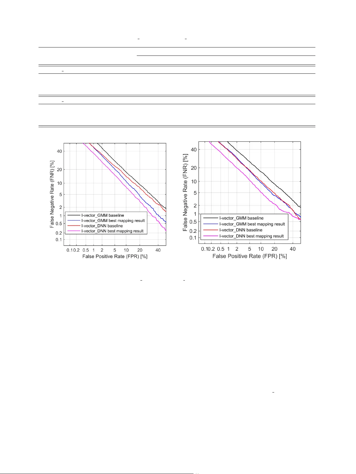
J. Guo et al. / 00 (2018) 1–14 1 Deep neural network based i-v ector mapping for speaker v erification using short utterances Jinxi Guo a, ∗ , Ning Xu b , Kailun Qian a , Y ang Shi a , Kaiyuan Xu a , Y ingnian W u c , Abeer Alwan a a Department of Electrical and Computer Engineering, University of California, Los Angeles, CA, United States, 90095. b Snap Inc, V enice, CA, United States, 90063. c Department of Statistics, University of California, Los Angeles, CA, United States, 90095. Abstract T ext-independent speaker recognition using short utterances is a highly challenging task due to the large variation and content mismatch between short utterances. I-vector and probabilistic linear discriminant analysis (PLD A) based systems ha ve become the standard in speaker v erification applications, b ut they are less e ff ecti ve with short utterances. In this paper , we first compare two state-of-the-art univ ersal background model (UBM) training methods for i-vector modeling using full-length and short utter- ance ev aluation tasks. The two methods are Gaussian mixture model (GMM) based (denoted I-v ector GMM) and deep neural network (DNN) based (denoted as I-vector DNN) methods. The results indicate that the I-vector DNN system outperforms the I-vector GMM system under various durations (from full length to 5 s). Howe ver , the performances of both systems de grade signif- icantly as the duration of the utterances decreases. T o address this issue, we propose two nov el nonlinear mapping methods which train DNN models to map the i-v ectors e xtracted from short utterances to their corresponding long-utterance i-vectors. The mapped i-vector can restore missing information and reduce the variance of the original short-utterance i-vectors. The proposed methods both model the joint representation of short and long utterance i-vectors: the first method trains an autoencoder first using con- catenated short and long utterance i-vectors and then uses the pre-trained weights to initialize a supervised re gression model from the short to long version; the second method jointly trains the supervised regression model with an autoencoder reconstructing the short utterance i-vector itself. Experimental results using the NIST SRE 2010 dataset sho w that both methods provide significant improv ement and result in a 24.51% relative improvement in Equal Error Rates (EERs) from a baseline system. In order to learn a better joint representation, we further in vestigate the e ff ect of a deep encoder with residual blocks, and the results indicate that the residual network can further improve the EERs of a baseline system by up to 26.47%. Moreover , in order to impro ve the short i-vector mapping to its long version, an additional v ector , which represents the a verage v alue of phoneme posteriors across frames, is also added to the input, and results in a 28.43% improv ement. When further testing the best-validated models of SRE10 on the Speaker In The Wild (SITW) dataset, the methods result in a 23.12% improv ement on arbitrary-duration (1-5 s) short-utterance conditions. K e ywor ds: speaker verification, short utterances, i-v ectors, DNNs, nonlinear mapping, joint modeling, autoencoder . 1. Introduction The i-vector based frame work has defined the state-of-the- art for text-independent speaker recognition. The i-vectors are extracted from either a Gaussian mixture model (GMM) based (Dehak et al., 2011) or a deep neural network (DNN) based system (Lei et al., 2011), and for the backend, probabilistic lin- ear discriminant analysis (PLD A) (Prince et al., 2007) has been ∗ Corresponding author Email Addr esses: lennyguo@g.ucla.edu (Jinxi Guo), ning.xu@snap.com (Ning Xu), kailunqian@ucla.edu (Kailun Qian), yangshi5@g.ucla.edu (Y ang Shi), kyxu@g.ucla.edu (Kaiyuan Xu), ywu@stat.ucla.edu (Y ingnian Wu), alwan@ee.ucla.edu (Abeer Alwan) widely used. The i-vector / PLD A system performs well if long (e.g. more than 30 s) enrollment and test utterances are avail- able, but the performance degrades rapidly when only limited data are av ailable (Kanagasundaram et al., 2011). T o address this issue, a range of techniques has been studied on di ff erent aspects of this problem (Poddar et al., 2017; Das and Prasanna, 2017). There has been a number of methods to model the v ariation of short utterance i-vectors. In Cumani (2014, 2015), a Full Posterior Distrib ution PLD A (FP-PLD A) is proposed to e xploit the cov ariance of the i-vector distribution, which improves the standard Gaussian PLDA (G-PLD A) model by accounting for the uncertainty of i-vector extraction. In Hasan et al. (2013), J. Guo et al. / 00 (2018) 1–14 2 the e ff ect of short utterance i-vectors on system performance was analyzed, and the duration v ariability was modeled as ad- ditiv e noise in the i-vector space. The work in Kanagasundaram et al. (2014) introduces a short utterance variance normalization technique and a short utterance variance modeling approach at the i-vector feature lev el; the technique makes use of the co- variance matrices of long and short i-vectors for normalization. Alternativ ely , se veral approaches hav e been proposed that lev erage phonetic information to perform content matching. The work in Li et al. (2016) proposes a GMM based subregion frame- work where speaker models are trained for each subregion de- fined by phonemes. T est utterances are then scored with sub- region models. In Chen et al. (2016), the authors use the lo- cal session variability v ectors estimated from certain phonetic components instead of computing the i-v ector from the whole utterance. Phonetic classes are obtained by clustering similar senones (group of triphones with similar acoustic properties) that are estimated from posterior probabilities of a DNN trained for phone state classification. Another approach was proposed in Sche ff er and Lei (2014) which matches the zero-order statis- tics of test and enrollment utterances using posteriors of each phone state before computing the i-vectors. In addition, a few studies ha ve focused on the role of feature extraction and score calibration. In Guo et al. (2016, 2017a), the authors proposed sev eral di ff erent methods (DNN and linear re- gression models) to estimate speaker-specific subglottal acous- tic features, which are more stationary compared to MFCCs, largely phoneme independent, and can alleviate the phoneme mismatch between training and testing utterances. In addition, Hasan et al. (2013) proposes a Quality Measure Function (QMF) which is a score-calibration mechanism that compensates for the duration mismatch in trial scores. Recently , several approaches have been proposed which use deep neural networks to learn speaker embedding from short- utterances. In Snyder et al. (2017), the authors use a neural network, which is trained to discriminate between a large num- ber of speakers, to generate fixed-dimensional speaker embed- ding, and the speaker embedding are used for PLDA scoring. In Zhang and K oishida (2017), the authors propose an end- to-end system which directly learns a speaker discriminative embedding using a triplet loss function and an Inception Net. Both methods show improvement o ver GMM-based i-vector systems. A few recent papers have focused on i-vector mapping, which maps the short utterance i-vector to its long version. In Kheder et al. (2016, 2018), the authors proposed a probabilistic ap- proach, in which a GMM-based joint model between long and short utterance i-vectors was trained, and a minimum mean square error (MMSE) estimator was applied to transform a short i-vector to its long v ersion. Since the GMM-based mapping function is actually a weighted sum of linear functions, our previous research (Guo et al., 2017b) demonstrates that a pro- posed non-linear mapping using con v olutional neural networks (CNNs) outperforms the GMM-based linear mapping methods across di ff erent conditions. The CNN-based mapping methods use unsupervised learning to re gularize the supervised regres- sion model, and result in significant performance improvement. This paper is an extension of our aforementioned work in Guo et al. (2017b) where we in vestigate neural network based non-linear mapping methods for i-vector mapping. Here, we first compare and analyze the performance of both GMM- and DNN- based i-vector systems with short-utterance ev aluation tasks. Based on the results which show that I-vector DNN sys- tems outperform I-vector GMM systems across durations, we first in vestigate our proposed non-linear i-vector mapping meth- ods using I-vector DNN systems. T wo nov el DNN-based i- vector mapping methods are proposed and compared. They both model the joint representation of short and long utterance i-vectors by making use of an autoencoder . The first method trains an autoencoder using concatenated short and long utterance i-vectors and then the pre-trained weights are used to perform fine-tuning for the supervised regression task which directly maps short to long utterances. By learn- ing a joint embedding of short and long utterances i-v ectors, the pre-trained autoencoder can help to initialize the weights at a desirable basin of the landscape of the loss function for the supervised training. Such pre-training prov es to be useful es- pecially when the training dataset is not large enough. Similar ideas of pre-training have been studied by Hinton et al. (2006) and Erhan et al. (2010). The second method jointly trains the supervised regression model with an autoencoder to reconstruct the short-utterance i-vector itself. The autoencoder here plays the role of a regu- larizer , which is important when the training dataset is not large enough and the dimensions of the input and output are relatively high. The fact that the autoencoder loss helps prev ent o verfit- ting has been observed in the machine learning literature. For example, in Rasmus et al. (2015); Zhang et al. (2016), a super- vised neural network is augmented with decoding pathw ays for reconstruction, and it is shown that the reconstruction loss helps improv e the performance of supervised tasks. More recently , a paper on CapNet (Sabour et al., 2017) introduces a decoder that plays a critical role in achie ving the state of the art performance on a classification task. W e further discuss several key factors of the proposed DNN mapping models in detail, including pre-training iteration, reg- ularization weights and encoder depth. The best model pro- vides more than 26.47% relative improv ement. W e also show that by adding additional phoneme information as input, we can achiev e further mapping improv ements (28.43%). W e apply the proposed mapping methods to di ff erent durations of e valuation utterances to represent real-life situations, and the results show their e ff ectiv eness across all conditions. The mapping results for both I-vector GMM and I-v ector DNN systems are com- pared, and show significant improvement for both systems. In the end, in order to sho w the generalization of the proposed methods, we apply the best-validated models of SRE10 (Mar - tin and Greenberg, 2010) dataset to the Speaker In The W ild (SITW) dataset (McLaren et al., 2015), which also sho w con- siderable improv ement (23.12%). This paper is structured as follo ws. Section 2 describes the state-of-the-art i-v ector / PLD A speaker verification systems. Section 3 analyzes the e ff ect of utterance duration on i-vectors and introduces the proposed DNN-based i-vector mapping meth- J. Guo et al. / 00 (2018) 1–14 3 ods in detail. Section 4 presents the experimental set-up. Ex- perimental results and analysis of the proposed techniques are presented in Section 5. Section 6 discusses mapping e ff ects, and finally , in Section 7, major conclusions are presented. 2. I-vector based speaker verification systems As mentioned earlier, the state-of-the-art te xt-independent speaker v erification system is based on the i-v ector framew ork. In these systems, a univ ersal background model (UBM) is used to collect su ffi cient statistics for i-vector extraction, and a PLD A backend is adopted to obtain the similarity scores between i- vectors. There are two di ff erent ways to model a UBM: us- ing unsupervised-trained GMMs or using a DNN trained as a senone classifier . Therefore, we will introduce both the I- vector GMM and I-vector DNN systems as well as PLD A mod- eling. 2.1. I-vector GMM system The i-vector representation is based on the total variability modeling concept which assumes that speaker- and channel- dependent v ariabilities reside in a low-dimensional subspace, represented by the total v ariability matrix T . Mathematically , the speaker - and channel-dependent GMM supervector s can be modeled as: s = s 0 + T w (1) where s 0 is the speaker - and channel-independent superv ector , T is a rectangular matrix of low rank and w is a random vec- tor called the i-vector which has a standard normal distribution N (0 , I ). In order to learn the total variability subspace, the Baum- W elch statistics need to be computed for a giv en utterance, which are defined as: N c = X t P ( c | y t , Ω ) (2) F c = X t P ( c | y t , Ω ) y t (3) where N c and F c represents the zeroth and first order statistics, y t is the feature sample at time inde x t , Ω represent the UBM of C mixture components, c = 1 , ..., C is the Gaussian index and P ( c | y t , Ω ) corresponds to the posterior of mixture component c generating the vector y t . 2.2. I-vector DNN system As mentioned in the pre vious section, for an I-v ector GMM system, the posterior of mixture component c generating the vector y t is computed with a GMM acoustic model trained in an unsupervised fashion (i.e. with no phonetic labels). P ( c | y t , Ω ) ⇒ P ( c | y t , Θ ) (4) Howe ver , recently , inspired by the success of DNN acoustic models in automatic speech recognition (ASR), Lei et al. (2011) proposed a method which uses DNN senone (cluster of context- dependent triphones) posteriors to replace the GMM posteriors as illustrated in Eq.4, which leads to significant improvement in speaker verification. Θ represents the trained DNN model for senone classfication. The senone posterior approach uses ASR features to com- pute the class soft alignment and the standard speaker verifica- tion features for su ffi cient statistic estimation. Once su ffi cient statistics are accumulated, the training procedure is the same as in the previous section. In this paper, we use a state-of-the-art time delay neural network (TDNN) as in Peddinti et al. (2015) to train the ASR acoustic model. 2.3. PLD A modeling PLD A is a generative model of i-vector distributions for speaker verification. In this paper , we use a simplified v ari- ant of PLDA, termed as G-PLD A (Kenny et al., 2013), which is widely used by researchers. A standard G-PLDA assumes that the i-vector w i is represented by: w i = r + U x +  i (5) where, r is the mean of i-vectors, U defines the between-speaker subspace, and the latent v ariable x represents the speaker iden- tity and is assumed to have standard normal distrib ution. The residual term  i represents the within-speaker v ariability , which is normally distributed with zero mean and full co variance Σ 0 . PLD A based i-v ector system scoring is calculated using the log likelihood ratio (LLR) between a target and test i-vectors, denoted as w tar get and w te st . The likelihood ratio can be calcu- lated as follows: L LR = log P ( w tar get , w te st | H 1 ) P ( w tar get | H 0 ) P ( w te st | H 0 ) (6) where H 1 and H 0 denote the hypothesis that two i-vectors rep- resent the same speaker , and di ff erent speakers, respectiv ely . 3. Short-utterance speaker verification 3.1. The e ff ect of utterance durations on i-vector s Full-length i-vectors have relatively smaller variations com- pared with i-vectors extracted from short utterances (Poddar et al., 2017), because i-vectors of short utterances can vary consid- erably with changes in phonetic content. In order to show the variation changes between long and short utterance i-vectors, we first calculate the av erage diagonal covariance (denoted as σ m ) of i-vectors across all utterances of a gi ven speaker m and then calculate the mean (denoted as σ mean ) of the cov ariances ov er all speakers. σ m and σ mean are defined in Eqs.7-8 as: σ m = 1 N Σ N n = 1 T r(( w mn − ¯ w m )( w mn − ¯ w m ) T ) (7) σ mean = 1 M Σ M m = 1 σ m (8) where ¯ w m corresponds to the mean of the i-vectors belonging to speaker m . N represents the total number of utterances for speaker m , T r( . ) represents the trace operation, and M is total number of speakers. J. Guo et al. / 00 (2018) 1–14 4 T able 1: Mean variance of long and short utterances (from SRE and Switchboard dataset) i-vectors long utterance short utterance mean variance( σ mean ) 283 493 Fig. 1. Distribution of activ e speech length of the selected 40000 long utterances. In order to compare the σ mean for long and short utterance i-vectors, we choose around 4000 speakers with multiple long utterances (more than 2 mins durations and 100 s acti ve speech) from the SRE and Switchboard (SWB) datasets (in total around 40000 long utterances) and truncate each long utterances into multiple 5-10 s short utterances. W e plot the distribution of activ e-speech length (utterance length after v oice acti vity de- tection) across these 40000 long utterances in Fig. 1. The i- vectors are e xtracted for each short and long utterance using the I-vector DNN system, and T able 1 sho ws the mean v ari- ance σ mean across all speakers calculated from long and short utterance i-v ectors indi vidually . The mean of variances in the T able 1 indicates that short-utterance i-v ectors ha ve lar ger v ari- ation compared to those of long-utterance i-vectors. 3.2. DNN-based i-vector mapping In order to alleviate possible phoneme mismatch in text- independent short utterances, we propose sev eral methods to map short-utterance i-v ectors to their long version. This map- ping is a many-to-one mapping, from which we want to restore the missing information from the short-utterance i-vectors and reduce their variance. In this section, we will introduce and compare se veral novel DNN-based i-vector mapping methods. Our pilot experiments indicate that, if we train a supervised DNN to learn this map- ping directly , which is similar to the approaches in Bousquet and Rouvier (2017) , the improvement is not significant, due to ov er-fitting to the training dataset. In order to solve this problem, we propose two di ff erent methods which both model the joint representation of short and long utterance i-vectors by using an autoencoder . The decoder reconstructs the origi- nal input representation and forces the encoded embedding to learn a hidden space which represents both short and long ut- terance i-v ectors and thus can lead to a better generalization. The first is a two-stage method: using an autoencoder to first train a bottleneck representation of both long and short utter - ance i-v ectors, and then uses the pre-trained weights to perform a supervised fine-tuning of the model, which maps the short- utterance i-vector to its long version directly . The second is a single-stage method: jointly train the supervised regression model with an autoencoder to reconstruct the short i-vector . The final loss to optimize is a weighted sum of the supervised regression loss and the reconstruction loss. In the following subsections, we will introduce these two methods in detail. 3.2.1. D N N 1 (two-stage method): pre-tr aining and fine-tunning In order to find a good initialization of the supervised DNN model, we first train a joint representation of both short and long utterance i-vectors using an autoencoder . W e first concatenate the short i-vector w s and its long version w l into z , then the concatenated vector z is used to train an autoencoder with some specific constraints. The autoencoder learns the joint hidden representation of both short and long i-vectors, which leads to good initialization of the second-stage supervised fine-tuning. The autoencoder consists of an encoder and a decoder as illus- trated in Fig. 2. The encoder function h = f ( z ) learns a hid- den representation of input vector z , and the decoder function ˆ z = g ( h ) produces a reconstruction. The learning process is de- scribed as minimizing the loss function L ( z , g ( f ( z ))). In order to learn a more useful representation, we add a restriction on the autoencoder: constrain the hidden representation h to have a relati vely small dimension in order to learn the most salient features of the training data. For the encoder function f ( . ), we adopt options from sev- eral fully-connected layers to stacked residual blocks (He et al., 2016), in order to in vestigate the e ff ect of encoder depth. Each residual block has two fully-connected layers with a short-cut connection as sho wn in Fig. 3. By using residual blocks, we are able to train a very deep neural network without adding extra parameters. A deep encoder may help learn better hidden rep- resentations. For a decoder function g ( . ), we use a single fully connected layer with a linear regression layer , since it is enough to approximate the mapping from the learned hidden represen- tation h to the output vector . For the loss function, we use the mean square error criterion, which is k g ( f ( z )) − z k 2 . Once the autoencoder is trained, we use the trained DNN- structure and weights to initialize the supervised mapping. W e optimize the loss between the predicted long i-vector and the real long i-vector 1 N P N n = 1 k ˆ w l − w l k 2 as sho wn in Fig. 2. W e J. Guo et al. / 00 (2018) 1–14 5 Fig. 2. D N N 1 : two-stage training of i-v ector mapping. Left schema corresponds to the first-stage pre-training. A short-utterance i-vector w s and a corresponding long-utterance i-vector w l are first concate- nated into z . Then z is fed into an encoder f ( . ) to generate the joint embedding h . h is passed to the decoder g ( . ) to generate the recon- structed ˆ z , which is expected to be a concatenation of a reconstructed ˆ w s and ˆ w l . Right schema corresponds to the second-stage fine-tuning. The pre-trained weights in the first stage is used to initialize the su- pervised regression model from w s to w l . After training, the estimated i-vector ˆ w l is used for ev aluation. Fig. 3. Residual block. An input x is first passed into tw o hidden layers to get F ( x ) and it also goes through a short-cut connection, which skips the hidden layers and directly comes to the output. The final output of the residual block is a summation of F ( x ) and x . Fig. 4. DN N 2 : single-stage training of i-vector mapping. A short- utterance i-vector w s is passed to an encoder and the output of the encoder is first used to generate the estimated long-utterance i-vector ˆ w l and it is also fed into a decoder to generate the reconstructed short- utterance i-vector ˆ w s . The two tasks are optimized jointly . denote this method as D N N 1 . 3.2.2. D N N 2 (single-stage method): semi-supervised training The tw o-stage method mentioned in the previous section, needs to first train a joint representation using the autoencoder and then perform a fine-tuning to train the supervised mapping. In this section, we introduce another unified semi-supervised framew ork based on our previous work (Guo et al., 2017b) which can jointly train the supervised mapping with an autoen- coder to minimize the reconstruction error . The joint frame- work is motiv ated by the fact that by sharing the hidden rep- resentations among supervised and unsupervised tasks, the net- work generalizes better and it can also av oid using the two-stage training procedures and speed up training. This method is de- noted as D N N 2 . W e adopt the same autoencoder framework as mentioned in the pre vious section, which has an encoder and a decoder , but the input to the encoder here is the short-utterance i-vector w s . The output from the encoder will be connected to a linear regression layer to predict the long-utterance i-vector w l , and it will also be used to reconstruct the short-utterance i-v ector w s itself by inputing it into a decoder, which gi ves rise to the autoencoder structure. The entire framework is sho wn in Fig. 4. W e define a new objecti ve function to jointly train the net- work. Let us use ˆ w l and ˆ w s to represent the output from the supervised regression model and autoencoder respectiv ely . W e can define the objective loss function L tot al which combines the loss from the regression model and the autoencoder in a weighted fashion as: L tot al = (1 − α ) L r + α L a (9) where L r is the loss of regression model defined as L r ( w s , w l ; θ r ) = 1 N N X n = 1 k ˆ w l − w l k 2 (10) and L a is the loss of an autoencoder defined as: L a ( w s , w s ; θ a ) = 1 N N X n = 1 k ˆ w s − w s k 2 . (11) Moreov er , θ r and θ a are parameters of the regression model and autoencoder respectively , which are jointly trained and share the weights of the encoder layer . α is a scalar weight, which determines how much the reconstruction error is used to re g- ularize the supervised learning. The reconstruction loss of the autoencoder L a forces the hidden vector generated from the en- coder to reconstruct the short-utterance i-v ector w s in addition to predicting the target long-utterance i-vector w l , and helps prev ent the hidden vector from ov er-fitting w l . For testing, we only use the output from the re gression model ˆ w l as the mapped i-vector . 3.2.3. Adding phoneme information The variance of short utterances is mainly due to phonetic di ff erences. In order to aid the neural network to train this non- linear mapping, for a giv en utterance, we e xtract the senone J. Guo et al. / 00 (2018) 1–14 6 T able 2: Datasets used for developing I-v ector GMM and I-vector DNN systems I-vector GMM I-vector DNN UBM (3472) Switchboard, NIST 04, 05, 06, 08 Fisher English T (600) Switchboard, NIST 04, 05, 06, 08 Switchboard, NIST 04, 05, 06, 08 PLD A NIST 04, 05, 06, 08 NIST 04, 05, 06, 08 Fig. 5. I-vector mapping with additional phoneme information. A short-utterance i-v ector w s is concatenated with a phoneme vector p to generate the estimated long-utterance i-vectors ˆ w l . posteriors for each frame and calculate the mean posterior across frames as a phoneme vector , which is then appended to a short utterance i-vector as input (Fig. 5). The training procedure still follows the proposed joint modeling methods ( DN N 1 or DN N 2 ). The phoneme vectors are e xpected to help normalize the short-utterance i-vector , and provide extra information for this mapping. The phoneme vector p is defined as: p = 1 N N X t = 1 P ( c | y t , Θ ) (12) The posterior P ( c | y t , Θ ) is generated from the TDNN-based senone classifier , which was defined in Section 2.2. 4. Experimental set-up 4.1. I-vector baseline systems W e ev aluate our techniques using the state-of-the-art GMM- and DNN-based i-vector / G-PLD A systems using the Kaldi toolkit (Pov ey et al., 2011). 4.1.1. Configurations of I-vector GMM system For the I-vector GMM system, the first 20 MFCC coe ffi - cients (discarding the zeroth coe ffi cient) and their first and sec- ond order deriv atives are extracted from the detected speech segments after an energy-based voice acti vity detection (V AD). A 20 ms Hamming windo w , a 10 ms frame shift, and a 23 chan- nels filterbank are used. Uni versal background models with 3472 Gaussian components are trained, in order to hav e a fair comparison with the I-vector DNN system, whose DNN has 3472 outputs. Initial training consists of four iterations of EM using a diagonal cov ariance matrix and then an additional four iterations with a full-cov ariance matrix. The total variability subspace with lo w rank (600) is trained for fi ve iterations of EM. The back end training consists of i-vector mean subtraction and length normalization, followed by PLD A scoring. The UBM and i-vector extractor training data consist of male and female utterances from the SWB and NIST SRE datasets. The SWB data contains 1000 speakers and 8905 utterances of SWB 2 Phases II. The SRE dataset consists of 3805 speak ers and 36614 utterances from SRE 04, 05, 06, 08. The PLD A backends are trained only on the SRE data. The dataset infor- mation is summarized in T able 2. 4.1.2. Configurations of I-vector DNN system For the I-vector DNN system, a TDNN is trained using about 1,800 hours of the English portion of Fisher (Cieri et al., 2004). In the TDNN acoustic modeling system, a narrow temporal context is provided to the first layer and context width increases for the subsequent hidden layers, which enables higher levels of the network to learn greater temporal relationships. The fea- tures are 40 mel-filterbank features with a frame-length of 25 ms. Cepstral mean subtraction is performed ov er a window of 6 s. The TDNN has six layers, and a splicing configuration similar to those described in Peddinti et al. (2015). In total, the DNN has a left-context of 13 and a right-context of 9. The hidden layers use the p-norm (where p = 2) acti vation function (Zhang et al., 2014), an input dimension of 350, and an output dimension of 3500. The softmax output layer computes posteri- ors for 3472 triphone states, which is the same as the number of components for I-v ector GMM system. No fMLLR or i-vectors are used for speaker adaptation. The trained TDNN is used to create a UBM which directly models phonetic content. A supervised-GMM with full-cov ariance is created first to initialize the i-vector extractor based on TDNN posteriors and speaker recognition features. T raining the T ma- trix also requires TDNN posteriors and speaker recognition fea- tures. During i-vector extraction, the only di ff erence between this and the standard GMM-based systems is the model used to compute posteriors. In the I-v ector GMM system, speaker recognition features are selected using a frame-lev el V AD, how- ev er , in order to maintain the correct temporal context, we can- not remove frames from the TDNN input features. Instead, the V AD results are used to filter out posteriors corresponding to non-speech frames. 4.1.3. Evaluation databases W e first ev aluate our systems on condition 5 (extended task) of SRE10 (Martin and Greenber g, 2010). The test consists of J. Guo et al. / 00 (2018) 1–14 7 T able 3: Baseline results for I-vector GMM and I-vector DNN systems under full-length and short-length utterances conditions reported in terms of EER, Relativ e Improv ement (Rel Imp), minDCF . Female Male EER (Rel Imp) DCF08 / DCF10 EER (Rel Imp) DCF08 / DCF10 Full-length condition I-vector GMM 2.2 0.011 / 0.043 1.7 0.008 / 0.036 I-vector DNN 1.4 (36.36%) 0.005 / 0.022 0.8 (52.94%) 0.003 / 0.017 10 s-10 s condition I-vector GMM 13.8 0.063 / 0.097 13.3 0.057 / 0.099 I-vector DNN 12.2 (11.59%) 0.054 / 0.093 10.2 (23.31%) 0.048 / 0.095 5 s-5 s condition I-vector GMM 21.7 0.083 / 0.099 20.4 0.080 / 0.100 I-vector DNN 19.9 (8.29%) 0.078 / 0.099 17.0 (16.67%) 0.072 / 0.100 con versational telephone speech in enrollment and test utter- ances. There are 416119 trials, over 98% of which are nontar- get comparisons. Among all trials, 236781 trials are for female speakers and 179338 trials are for male speakers. For short- utterance speaker verification tasks, we extracted short utter- ances which contain 10 s and 5 s speech (after V AD) from con- dition 5 (extended task). W e train the PLD A and ev aluate the trials in a gender-dependent w ay . Moreov er , in order to v alidate our proposed methods in real conditions and demonstrate the models’ generalization, we use SITW , a recently published speech database (McLaren et al., 2015). The SITW speech data was collected from open-source media channels with considerable mismatch in terms of au- dio conditions. W e designed an arbitrary-length short-utterance task using SITW dataset to represent real-life conditions. W e show the ev aluation results using the best-performed models validated on SRE10 dataset. 4.2. I-vector mapping training In order to train the i-vector mapping model, we selected 39754 long utterances, each ha ving more than 100 s of speech after V AD, from the de velopment dataset. For each long utter- ance, we used a 5 s or 10 s windo w to truncate the utterance, and the shift step is half of window size (2.5 s or 5 s). W e applied the aforementioned procedures to all long utterances, and in the end we got 1.2M 10 s utterances and 2.4M 5 s utter- ances. All short-utterance i-v ector together with its correspond- ing long-utterance i-vector are used as training pairs for DNN- based mapping models. W e train the mapping models for each gender separately and e valuate the model in a gender-dependent way . For the proposed two DNN-based mapping models, we use the same encoder and decoder configurations. For the encoder , we first use two fully-connected layers. The first layer has 1200 hidden nodes and the second layer has 600 hidden nodes which is a bottleneck layer (1.44M parameters in total). In order to in vestigate the depth of the encoder , we design a deep structure with two residual blocks and a bottleneck layer , in a total of 5 layers. Each residual block (as defined in Section 3.2.1) has two fully connected layers with 1200 hidden nodes and the bottle- neck layer has 600 hidden nodes (5.76M parameters in total). For the decoder , we always use one fully-connected layer (1200 hidden nodes) with a linear output layer (1.44M parameters in total). In order to add phoneme information for i-vector mapping, phoneme vectors are generated for each utterance by taking the av erage of the senone posteriors across frames. Since the phoneme v ectors ha ve a di ff erent v alue range compared with i-vectors, it will de-emphasize their e ff ect for training the map- ping. Therefore we scale up the phoneme vector values by a factor of 500, in order to match the range of i-vector values. The up-scaled phoneme v ector is then concatenated with short- utterance i-vector for i-v ector mapping. All neural networks are trained using the Adam optimiza- tion strategy (Kingma et al., 2014) with mean square error cri- terion and exponentially decaying learning rate starting from 0.001. The networks are initialized with the Xavier initializer (Glorot and Bengio, 2010), which is better than the Gaussian initializer as shown in Guo et al. (2017b). The relu activ ation function is used for all layers. For each layer , before passing the tensors to the nonlinearity function, a batch normalization layer (Io ff e and Sze gedy, 2015) is applied to normalize the ten- sors and speed up the conv ergence. For the combined loss of DN N 2 , we set equal weights ( α = 0.5) for both re gression and autoencoder loss for initial experiments. The shu ffl ing mecha- nism is applied on each epoch. The T ensorflow toolkit (Abadi et al., 2016) is used for neural network training. 5. Evaluation results and analysis 5.1. I-vector baseline systems In this section, we present and compare two baseline sys- tems: a I-vector GMM system and a I-vector DNN system, with standard NIST SRE 10 full-length condition and truncated 10 s-10 s and 5 s-5 s conditions. T able 3 shows the equal error rate (EER) and minimum de- tection cost function (minDCF) of the tw o baseline systems un- der full-length ev aluation condition and truncated short-length J. Guo et al. / 00 (2018) 1–14 8 T able 4: Results for baseline (I-v ector DNN), matched-length PLD A training, LDA dimension reduction, DNN direct mapping and proposed DNN mapping in the 10 s-10 s condition. Female Male EER (Rel Imp) DCF08 / DCF10 EER (Rel Imp) DCF08 / DCF10 baseline 12.2 0.054 / 0.093 10.2 0.048 / 0.095 matched length PLD A 11.3 (7.38%) 0.052 / 0.093 9.4 (7.84%) 0.043 / 0.095 LD A 150 11.6 (5.00%) 0.052 / 0.093 9.8 (3.92%) 0.047 / 0.093 DNN direct mapping 10.5 (13.93%) 0.054 / 0.096 9.7 (4.90%) 0.047 / 0.093 DNN1 mapping 9.5 (22.13%) 0.047 / 0.091 7.7 (24.51%) 0.039 / 0.090 DNN2 mapping 9.5 (22.13%) 0.047 / 0.091 7.7 (24.51%) 0.039 / 0.089 ev aluation conditions. Both DCF08 and DCF10 (defined in NIST 2008 and 2010 ev aluation plan) are shown in the table. From the table, we can observ e that the I-vector DNN system giv es significant improv ement under the full-length condition compared with I-vector GMM system and achieved a max of 52.94% relativ e improvement for the male condition, which is consistent with previous reported results (Snyder et al., 2015). This is mainly because the DNN model provides phonetically- aware class alignments, which can better model speakers. The good performance is also due to the strong TDNN-based senone classifier , which makes the alignments more accurate and ro- bust. When both systems were e valuated on the truncated 10 s-10 s, 5 s-5 s e valuation conditions, the performances degrade significantly compared with the full-length condition. The main reason is that when the length of the e v aluation utterance is shorter , there is significant phonetic mismatch between utter- ances. Ho wev er , the performance of the I-vector DNN system still outperforms the I-v ector GMM system by 8%-24%, ev en though the improvement is not as big as the full-length condi- tion. From the table, we can also observe that the improvement is more significant for male speakers across all conditions. It may be the fact that phoneme classification is more accurate for male speakers, which could lead to a better phoneme-aw are speaker modeling. 5.2. I-vector mapping r esults In this section, we show and discuss the performance of the proposed algorithms when only short utterances are av ailable for ev aluation. Since from T able 3 we can observe better per- formance using I-vector DNN systems, we will mainly use the I-vector DNN system to in vestigate the mapping methods. W e first show the results on the 10 s-10 s condition. Previous work (Kheder et al., 2016; Guo et al., 2017b) high- lights the importance of duration matching in PLD A model train- ing. For instance when the PLDA is trained using long utter- ances and ev aluated on short utterances, there is degradation in speaker v erification performance compared to PLD A trained using matched-length short utterances. Therefore, we not only show our baseline results for the PLDA trained using the reg- ular SRE de velopment utterances, but also show the results for the PLD A condition using truncated matched-length short ut- terances. For other baseline comparison, we first apply dimension- ality reduction on i-v ectors using linear discriminant analysis (LD A) and reduce the dimension of i-vectors from 600 to 150. This value has been selected according to the results of pre vi- ous research (Cumani, 2016). LD A can maximize inter-speaker variability and minimize intra-speaker variability . W e train the LD A transformation matrix using the SRE dev elopment dataset, and then, perform the dimension reduction for all development utterances and train a new PLD A model. For ev aluation, all i- vectors are subjected to dimensionality reduction first and then we use the new PLDA model to get similarity scores. T o com- pare with another short-utterance compensation technique, we ev aluate the i-vector mapping methods proposed in Bousquet and Rouvier (2017), which use DNNs to train a direct map- ping from short-utterance i-v ectors to the corresponding long version. Similar to Bousquet and Rouvier (2017), we also add some long-utterance i-v ectors as input for regularization pur - poses. For our proposed DNN mapping methods, we first sho w the mapping results for both DN N 1 and DN N 2 with three hid- den layers. Note that for mapped i-vectors, we use the same PLD A as the baseline system to get similarity scores. W e fur- ther in vestigate the e ff ect of pretraining iterations for DN N 1 , the weight α of the reconstruction loss for D N N 2 and the depth of encoder , compare the results for di ff erent durations, and in- vestigate the e ff ect of additional phoneme information. W e also compare with mapping results for both I-vector GMM and I- vector DNN systems. In the end, we test the generalization of the trained models on the SITW dataset. T able 4 presents the results for re gular PLD A training con- dition (baseline), matched-length PLD A condition, LD A dime- tionality reduction method, DNN-based direct mapping method, DNN-based tw o-stage method ( D N N 1 ) and DNN-based single- stage method ( D N N 2 , α = 0.5). W e observe that matched-length PLD A training gi ves considerable improv ement compared with non-matched PLD A training (baseline), which is consistent with previous work. When training the PLDA using short-utterance i-vectors, the system can capture the v ariance of short-utterance i-vectors. Using LDA to do dimentionality reduction also re- sults in some improv ement, since it reduces the variance of the i-vectors. DNN-based direct mapping giv es more improvement for female speakers (13.93%) compared with male speakers (5%) in terms of EERs, and it may be due to the fact that more J. Guo et al. / 00 (2018) 1–14 9 T able 5: DNN-based mapping results using DNNs with di ff erent depths in the 10 s-10 s condition. Female Male EER (Rel Imp) DCF08 / DCF10 EER (Rel Imp) DCF08 / DCF10 baseline 12.2 0.054 / 0.093 10.2 0.048 / 0.095 DNN1 mapping (3 layer) 9.5 (22.13%) 0.047 / 0.091 7.7 (24.51%) 0.039 / 0.090 DNN2 mapping (3 layer) 9.5 (22.13%) 0.047 / 0.091 7.7 (24.51%) 0.039 / 0.089 DNN1 mapping (6 layer + residual block) 9.1 (25.41%) 0.046 / 0.091 7.5 (26.47%) 0.038 / 0.089 DNN2 mapping (6 layer + residual block) 9.3 (23.77%) 0.047 / 0.091 7.6 (25.49%) 0.038 / 0.089 training data is a vailable for female speak ers and thus the ov er- fitting problem is less severe for females. In the last two rows, we show the performance of our proposed DNN-based mapping methods on short-utterance i-vectors. From the results, we can observe that they both result in significant improvements over the baseline for both the EER and minDCF metrics, and they also outperform the other short-utterance compensation meth- ods by a large mar gin. DN N 1 and D N N 2 methods ha ve compa- rable performance, which prove the importance of learning joint representation of both short and long utterance i-vectors. The proposed methods outperform the baseline system by 22.13% for female speakers and improve the male speaker baseline by 24.51%. One of the advantages using DN N 2 is that the uni- fied framework av oids using the two-stage training procedure, which speeds up the training. 5.2.1. E ff ect of pr e-training for D N N 1 In this section, we will sho w how first-stage pre-training in- fluences the second-stage mapping training for DN N 1 . W e hav e in vestigated the number of training iterations used for first-stage pre-training from 10000-50000. What we find interesting is that when the number of training iterations is small, the second stage fine-tuning will ov er-fit the data, but when the number of train- ing iterations is large, the fine-tuning results are not optimal. In the end, 25000 iterations was a roughly good initialization for second stage fine-tuning. This indicates that the number of iter - ations for unsupervised training does influence the second-stage supervised training. Fig. 6. EER as a function of reconstruction loss α for D N N 2 . 5.2.2. E ff ect of r econstruction loss for DN N 2 In this section, we in vestigate the impact of the weights for the reconstruction loss in D N N 2 . W e set α = { 0.1,0.2,0.5, 0.8,0.9 } . Since the weight of regression loss is 1 − α , the lar ger α is, the less weight will be assigned to regression loss. Fig. 6 shows the EER for female speakers as a function of the weights assigned to reconstruction loss. The reconstruction loss is clearly important for this joint learning framework. It forces the net- work to learn the original representations for short utterances, which can re gularize the regression task and generalize better . The optimal reconstruction weight is α = 0.8, which indicates that the reconstruction loss is ev en more important for this task. Hence, it appears that unsupervised learning is very crucial for a speaker recognition task. 5.2.3. E ff ect of encoder depth The depth of neural network has been proven to be impor - tant for network performance. Adding more layers will make the network more e ffi cient and powerful to model data. There- fore, as discussed in Section 4.2, we will compare a shallo w (2- layer) and a deep (5-layer) encoder for both DN N 1 and DN N 2 . It’ s well known that training a deep model su ff ers a lot from gradient v anishing / exploding problems and also it can be easily stuck into local minimum points. Therefore, we use two meth- ods to alleviate this problem. Firstly , as stated in Section 4.2, we use a normalized initialization (Xavier initialization) and a batch normalization layer to normalize the intermediate hidden output. Secondly , we apply residual learning, which uses se v- eral residual blocks (defined in Section 3.2.1) with no extra parameter compared with regular fully-connected layers. The residual blocks will make the information flow between layers easy and enable v ery smooth forward / backw ard propagation, which makes it feasible to train deep networks. T o our knowl- edge, this is one of the first studies to in vestig ate the e ff ect of residual networks for auto-encoder and unsupervised learning. Here, for the deep encoder , we use 2 residual blocks and 1 fully- connected bottleneck layer (in total 5 layers). For the decoder , we use a single hidden layer with a linear regression output layer . From T able 5, we can observe that a deep encoder does re- sult in improv ements compared with a shallo w encoder . Es- pecially for D N N 1 , the residual networks give a 25.41% rela- tiv e improvement for female speakers and 26.47% relativ e im- prov ement for male speakers. The results indicate that learning a good joint representation of both short and long utterance i- J. Guo et al. / 00 (2018) 1–14 10 T able 6: DNN-based mapping results with additional phoneme information in the 10 s-10 s condition. Female Male EER (Rel Imp) DCF08 / DCF10 EER (Rel Imp) DCF08 / DCF10 baseline 12.2 0.054 / 0.093 10.2 0.048 / 0.095 DNN mapping (best) 9.1 (25.41%) 0.046 / 0.091 7.5 (26.47%) 0.038 / 0.089 DNN mapping (best) + phoneme info 8.9 (27.05%) 0.046 / 0.090 7.3 (28.43%) 0.037 / 0.090 T able 7: DNN-based mapping results with di ff erent utterance durations. Female Male EER (Rel Imp) DCF08 / DCF10 EER (Rel Imp) DCF08 / DCF10 10 s-10 s baseline 12.2 0.054 / 0.093 10.2 0.048 / 0.095 DNN mapping (best) 9.1 (25.41%) 0.046 / 0.091 7.5 (26.47%) 0.038 / 0.089 5 s-5 s baseline 19.9 0.078 / 0.099 17.0 0.072 / 0.100 DNN mapping (best) 14.8 (25.62%) 0.067 / 0.099 13.5 (20.59%) 0.061 / 0.100 mix baseline 17.8 0.068 / 0.097 14.4 0.061 / 0.100 DNN mapping (best) 13.2 (25.84%) 0.061 / 0.097 11.8 (18.06%) 0.053 / 0.096 vectors is very beneficial for this supervised mapping task, and the deep encoder can help learn a better bottleneck joint em- bedding. The deep encoder can also decrease the amount of training data needed to model the non-linear function, which can also alle viate the over -fitting problem. In order to show the e ff ect of residual short-cuts, we performed experiments using a deep encoder without short-cut connections, and the system resulted in e ven w orse performance compared with the shallow encoder . Therefore, residual blocks with short-cut connections are very crucial for deep neural network training, since it alle- viates the hard optimization problems of deep networks. 5.2.4. E ff ect of adding phoneme information In this section, we show the results when adding phoneme vector (mean of phoneme posteriors across frames) with short- utterance i-v ectors to learn the mapping. W e will inv estigate the e ff ect of adding phoneme information based on the best performed DNN-mapping structures. From T able 6, we can observe that when adding phoneme vector , the EER further im- prov es to 8.9% for female speakers and 7.3% for male speakers from the previous best DNN-mapping results. It achiev es the best results for this task. The results prove the hypothesis that adding a phoneme vector can help the neural network reduce the v ariance of short-utterance i-vectors, which will lead to bet- ter and more generalizable mapping results. In Section 5.4, we will also show the e ff ect of adding phoneme vectors to GMM- i-vectors. 5.3. Results with di ff er ent durations In this section, the results for di ff erent durations of ev alu- ation utterances are listed. T able 7 shows the baseline and the best mapping results for 10 s-10 s, 5 s-5 s and mixed duration conditions. From the table, we can observe that the proposed methods gi ve significant improv ements for both 10 s-10 s and 5 s-5 s conditions, which indicates that the proposed method gen- eralizes to di ff erent durations. In real applications, ho wev er , the duration of short utterances can not be controlled, therefore we train the mapping using the i-vectors generated from mix ed 10 s and 5 s utterances and show the results also on a mix ed-duration ev aluation task (mixed of 5 s and 10 s). From T able 7, we can see that the baseline results for the mixed condition range be- tween the EER results of 10 s-10 s and the 5 s-5 s e v aluation tasks. The proposed mapping algorithms can model i-vectors extracted from v arious durations, and thus gi ve consistent im- prov ement as shown in the table. 5.4. Comparison of mapping r esults for both I-vector GMM and I-vector DNN systems In the previous sections, we only show the mapping exper- iments for I-vector DNN system, therefore, in this section, we will show the mapping results for the I-vector GMM system. In Section 5.1, we show that for the baseline results, I-vector DNN system outperforms the I-v ector GMM system, b ut it is also in- teresting to compare the results after mapping. From T able 8 we observe that the proposed mapping methods gi ve significant im- prov ement for both systems. After mapping, the I-vector DNN systems still outperform the I-vector GMM systems and the superiority of I-vector DNN systems is even more significant. W e also compare the mapping results when adding phoneme vectors. The table sho ws that the e ff ect of adding phoneme information is more significant for GMM-i-vectors and it can achiev e as much as a 10% relati ve improv ement on the best DNN mapping baseline. The reason is that DNN-i-vectors al- ready contain some phoneme information, while GMM-i-vectors J. Guo et al. / 00 (2018) 1–14 11 T able 8: Results for I-vector GMM and I-vector DNN systems in the 10 s-10 s conditions. Female Male EER (Rel Imp) DCF08 / DCF10 EER (Rel Imp) DCF08 / DCF10 I-vector GMM baseline 13.8 0.063 / 0.097 13.3 0.057 / 0.099 DNN mapping (best) 11.0 (20.29%) 0.054 / 0.095 10.6 (20.30%) 0.051 / 0.096 DNN mapping (best) + phoneme info 10.4 (24.64%) 0.053 / 0.094 9.6 (27.82%) 0.048 / 0.096 I-vector DNN baseline 12.2 0.054 / 0.093 10.2 0.048 / 0.095 DNN mapping (best) 9.1 (25.41%) 0.046 / 0.091 7.5 (26.47%) 0.038 / 0.089 DNN mapping (best) + phoneme info 8.9 (27.05%) 0.046 / 0.090 7.3 (28.43%) 0.037 / 0.090 (a) female speakers (b) male speakers Fig. 7. DET curves for the mapping results of I-vector GMM and I-vector DNN systems under 10 s-10 s conditions. Left figure corresponds to female speakers and right one corresponds to male speakers. do not hav e clear phoneme representation. Therefore GMM-i- vectors can benefit more from adding phoneme vectors. In the end, we summarize the baseline and the best mapping results for both systems in Fig. 7. The DET (Detection Error Trade- o ff ) curves are presented for both female and male speakers. The figures indicate that the proposed mapping algorithms gi ve significant improv ement from the baseline across all operation points. 5.5. P erformance on the SITW database In the previous experiments, we sho w the performance of our proposed DNN-mapping methods on NIST data. In this subsection, we apply our technique on the recently published database SITW which contains real-world audio files collected from open-source media channels with considerable mismatch conditions. In order to generate a large number of random- duration short utterances, we first combined the de v and ev al datasets and then selected 207 utterances from relatively clean condition. W e truncated each of 207 utterances into se veral non-ov erlapped short utterances with duration 5 s, 3.5 s, 2.5 s (including both speech and non-speech portions). In the end, a total number of 1836 utterances was generated. W e plot the distribution of active speech length across these 1836 utter- ances in Fig. 8. From the figure, we can observe that activ e speech length varies between 1 s-5 s across those short utter - ances. Therefore, we can use these short utterances to design trials, which represent real-w orld conditions (arbitrary-length short utterances). In total, we designed 664672 trials for our arbitrary-length short-utterance speaker verification task. For each short utterance, we first do wn-sampled the audio files to 8 kHz sampling rate, and then e xtracted the i-vectors using the pre viously trained I-vector DNN system introduced in Section 4.1. For PLDA scoring, we use the same PLDA in Section 4.1, which is trained using the SRE dataset. For i-vector mapping, we use the best-validated models on SRE10 dataset (5 s condition) to apply to the SITW dataset. Ev aluation results of EERs and minDCFs are show in T able 9. From the table, we can observe that the best models v alidated on SRE10 dataset gen- J. Guo et al. / 00 (2018) 1–14 12 T able 9: DNN-based mapping results on SITW using arbitrary durations of short utterances. Female Male EER (Rel Imp) DCF08 / DCF10 EER (Rel Imp) DCF08 / DCF10 Arbitrary durations baseline 17.3 0.061 / 0.089 12.0 0.046 / 0.083 DNN mapping (best models from SRE10) 13.3 (23.12%) 0.050 / 0.086 9.4 (21.67%) 0.039 / 0.078 Fig. 8. Distribution of activ e speech length of truncated short utter - ances in the SITW database. eralize well to the SITW dataset, which gi ve a 23.12% relative improv ement of EERs for female speakers and a 21.67% rela- tiv e improvement for male speakers. The results also indicate that the proposed methods can be used in real-life conditions, such as smart home and forensic related applications. 6. Mapping e ff ects In order to in vestigate the e ff ect of the proposed i-vector mapping algorithms, we first calculate the av erage square Eu- clidean distance between short and long utterance i-vector pairs on the SRE10 ev aluation dataset before and after mapping. The av erage mean square Euclidean distance D sl between short and long utterance i-vector is defined as follo w: D sl = 1 N Σ N s = 1 ( Σ L i = 1 ( w s ( i ) − w l ( i )) 2 ) (13) where w s and w l represent the short-utterance and long-utterance i-vector respecti vely , L is the length of i-vectors and N is num- ber of short and long i-vector pairs. W e compare the D sl values for 10 s and 5 s short-utterance i-vectors and also the mapped 10 s and 5 s short-utterance i- vectors for female and male speakers in T able 10. From the ta- ble, we observ e that, after mapping, the mapped short-utterance i-vectors hav e considerably smaller D sl compared to the ones before mapping. After mapping, the D sl in the 10 s condition is smaller compared with the 5 s condition. Moreov er , we calculate and compare the J-ratio (Fukunaga , 1990) of the short-utterance i-vectors from SRE10 before and after mapping in T able 11, which measures the ability of speaker separation. Given i-vectors for M speakers, the J-ratio can be computed using Eqs.14-16: S w = 1 M Σ M s = 1 R i (14) S b = 1 M Σ M s = 1 ( w i − w o )( w i − w o ) T (15) J = T r(( S b + S w ) − 1 S b ) (16) where S w is the within-class scatter matrix, S b is the between- class scatter matrix, w i is the mean i-vector for the i th speaker , w o is the mean of all w i s, and R i is the co variance matrix for the i th speaker (note that a higher J-Ratio means better separation). From T able 11, we can observe that the mapped i-vectors hav e considerably higher J-ratios compared with original short- utterance i-vectors for both 5 s and 10 s conditions. These results indicate that the proposed DNN-based map- ping methods can generalize well to unseen speakers and utter - ances, and improv e the speaker separation ability of i-vectors. 7. Conclusions In this paper , we show how the performance of both GMM and DNN-based i-vector speaker verification systems degrade rapidly as the duration of the ev aluation utterances decreases. This paper explains and analyzes the reasons of the degrada- tion and proposes se veral DNN-based techniques to train a non- linear mapping from short-utterance i-vectors to their long ver- sion, in order to improv e the short-utterance e valuation perfor- mance. T wo DNN-based mapping methods ( D N N 1 and D N N 2 ) are proposed and the y both model the joint representations of short- utterance and long-utterance i-vectors. For D N N 1 , an auto- encoder is trained first using concatenated short- and long- ut- terance i-vectors in order to learn a joint hidden representation, and then the pre-trained DNN is fine tuned by a supervised map- ping from short to long i-vectors. DN N 2 adopts a unified struc- ture, which jointly trains the supervised regression task with an auto-encoder since auto-encoders can directly re gularize the non-linear mapping between short and long utterances. The unified structure simplifies the training procedure and can also learn a generalized non-linear function. Both D N N 1 and D N N 2 result in significant improv ement ov er the short-utterance e valuation baseline for both male and female speakers, and they also outperform other short-utterance J. Guo et al. / 00 (2018) 1–14 13 T able 10: Square Euclidean distance ( D sl ) between short and long utterance i-vector pairs from SRE10 before and after mapping. D sl 10 s 5 s original mapped original mapped female 558.3 306.8 618.8 352.1 male 493.2 308.8 556.1 346.5 T able 11: J-ratio for short-utterance i-vectors from SRE10 before and after mapping. J-ratio 10 s 5 s original mapped original mapped female 87.96 92.97 82.73 85.18 male 85.23 90.25 80.41 84.39 compensation techniques by a large margin. After performing a t-test (p < 0.001), the results indicate that all the improv ements are statistically significant. W e study several key factors of DNN models and conclude the follo wing: 1) for the two-stage trained DNN model ( DN N 1 ), the number of iterations for un- supervised training in the first stage is important for second- stage supervised training; 2) for the semi-supervised trained DNN model ( D N N 2 ), unsupervised training plays a more im- portant role than supervised training in a speaker verification task; 3) by increasing the depth of the neural networks using residual blocks, we can alleviate the hard optimization prob- lem of deep neural networks and obtain an improv ement com- pared with a shallow network, especially for D N N 1 ; 4) adding phoneme information can aid in learning the non-linear map- ping and provide further performance improvement, and the ef- fect is more significant for GMM i-vectors; 5) the proposed DNN-based mapping methods work well for short utterances with di ff erent and mixed durations; 6) the proposed models can also impro ve both I-vector GMM and I-vector DNN systems and after mapping, a I-v ector DNN system still performs better than a I-vector GMM system; and 7) the best-validated models of SRE10 generalize well to the SITW dataset and give signifi- cant improv ement for arbitrary-length short utterances. References Dehak, N., K enny , P . J., Dehak, R., Dumouchel, P ., Ouellet, P . 2011. Front- end factor analysis for speaker verification, IEEE Transactions on Audio, Speech, and Language Processing, 19(4), pp. 788–798. Lei, Y ., Sche ff er , N., Ferrer, L., McLaren, M. 2014. A nov el scheme for speaker recognition using a phonetically-aware deep neural network, ICASSP 2014, pp. 1695–1699. Kanagasundaram, A., V ogt, R., Dean, D., et al, 2011. I-vector based speaker recognition on short utterances, in Proc. of Interspeech 2011, pp. 2341– 2344. Poddar , A., Sahidullah, M., Saha, G., 2017. Speaker v erification with short utterances: a re view of challenges, trends and opportunities, in IET Biomet- rics, 2018, vol. 7, no. 2, pp. 91–101. Das, R. K., Prasanna, S. M., 2017. Speaker verification from short utterance perspectiv e: a revie w , IETE T echnical Review , 2017, pp. 1–19. Prince, S. J., Elder, J. H., 2007. Probabilistic linear discriminant analysis for inferences about identity , ICCV 2007, pp. 1–8. Cumani, S., PIchot, O, Laface, P , 2015. On the use of i-vector posterior distri- butions in probabilistic linear discriminant analysis, IEEE T ransactions on Audio, Speech and Language Processing, 22(4), pp. 846–857. Cumani, S., 2015. Fast scoring of full posterior PLD A models, IEEE Transac- tions on Audio, Speech and Language Processing, 23(11), pp. 2036–2045. Cumani, S., Laface, P , 2016. I-vector transformation and scaling for PLDA based speaker recognition, In Proc. of Odyssey 2016, pp. 39–46. Hasan, T ., Saeidi, R., Hansen, J. H., et al, 2013. Duration mismatch com- pensation for i-vector based speaker recognition systems, ICASSP 2016, pp. 7663–7667. Kanagasundaram, A., Dean, D., Sridharan, S., et al, 2014. Impro ving short ut- terance i-vector speak er v erification using utterance v ariance modeling and compensation techniques, Speech Communication, 59:69–82. Li, L., W ang, D., Zhang, C., Zheng, T . Z., 2016. Improving short utterance speaker recognition by modeling speech unit classes, IEEE Transactions on Audio, Speech, and Language Processing, 24(6), pp. 1129–1139. Chen, L., Lee,K. A., Chng, E. S., Ma, B., Li, H, Dai, L. R., 2016. Content- aware local v ariability vector for speaker verification with short utterance, ICASSP 2016, pp. 5485–5489. Sche ff er , N. and Lei, Y ., 2014. Content matching for short duration speaker recognition, in Proc. of Interspeech 2014, pp. 1317–1321. Snyder , D., Garcia-Romero, D., Povey , D., Khudanpur , S. 2017. Deep neural network embeddings for text-independent speaker verification, in Proc. of Interspeech 2017, pp. 999–1003. Zhang, C., Koishida, K., 2017. End-to-end text-independent speaker verifi- cation with triplet loss on short utterances, in Proc. of Interspeech 2017, pp. 1487–1491 Guo, J., Y eung, G., Muralidharan, D., Arsikere, H., Afshan, A., Alwan, A., 2016. Speak er verification using short utterances with DNN-Based estima- tion of subglottal acoustic features, in Proc. of Interspeech 2016, pp. 2219– 2222. Guo, J., Y ang, R., Arsikere, H., Alwan, A., 2017. Robust speak er identification via fusion of subglottal resonances and cepstral features, the Journal of the Acoustical Society of America, 141(4), EL, pp. 420–426. Kheder , W . B., Matrouf, D., Ajili, M., Bonastre, J. F . , 2016. Probabilis- tic approach using joint long and short session i-V ectors modeling to deal with short utterances for speaker recognition, in Proc. of Interspeech 2016, pp. 1830–1834. Kheder , W . B., Matrouf, D., Ajili, M., Bonastre, J. F . , 2018. A unified joint model to deal with nuisance variabilities in the i-V ector space, IEEE / A CM T ransactions on Audio, Speech, and Language Processing, 26(3), pp. 633– 645. Ma, J., Sethu, V ., Ambikairajah, E., Lee, K. A. 2017. Incorporating local acous- tic variability information into short duration speaker verification, in Proc. of Interspeech 2017, pp. 1502–1506. J. Guo et al. / 00 (2018) 1–14 14 Bhattacharya, G., Alam, J., Kenny , P . 2017. Deep Speaker embeddings for short-Duration speaker verification, in Proc. of Interspeech 2017, pp. 1517– 1521. He, K., Zhang, X., Ren, S., Sun, J. 2016. Deep residual learning for image recognition, in Proc. of the IEEE conference on computer vision and pattern recognition 2016, pp. 770–778. Guo, J., Nookala, U. A., Alwan, A. 2017. CNN-based joint mapping of short and long utterance i-vectors for speaker v erification using short utterances, in Proc. of Interspeech 2017, pp. 3712–3716. Hinton, G. E., Osindero, S., T eh, Y . W . 2006. A fast learning algorithm for deep belief nets, Neural computation 2006, 18(7), pp 1527–1554. Erhan, D., Bengio, Y ., Courville, A., Manzagol, P . A., V incent, P ., Bengio, S. 2010. Why does unsupervised pre-training help deep learning? Journal of Machine Learning Research 2010, 11(Feb), pp. 625–660. Rasmus, A., Berglund, M., Honkala, M., V alpola, H., Raiko, T . 2015 Semi- supervised learning with ladder networks, Adv ances in Neural Information Processing Systems 2015, pp. 3546-3554. Zhang, Y ., Lee, K., Lee, H. 2016 Augmenting supervised neural netw orks with unsupervised objecti ves for large-scale image classification, International Conference on Machine Learning 2016, pp 612–621. Sabour , S., Frosst, N., Hinton, G. E. 2017. Dynamic routing between capsules, Advances in Neural Information Processing Systems 2017, pp 3859–3869. Bousquet, P . M., Rouvier , M. 2017. Duration mismatch compensation using four-co variance model and deep neural netw ork for speaker verification., in Proc. of Interspeech 2017, pp. 1547–1551. Kenn y , P ., Stafylakis, T ., Ouellet, P ., Alam, M. J., Dumouchel, P . 2013. PLD A for speaker v erification with utterances of arbitrary duration, ICASSP 2013, pp. 7649–7653 Cieri, C., Miller , D., W alker , K. 2004 The Fisher Corpus: a resource for the next generations of speech-to-T ext, in LREC V ol. 4, pp. 69–71 . Peddinti, V ., Pov ey , D., Khudanpur , S. 2015. A time delay neural network ar- chitecture for e ffi cient modeling of long temporal contexts, in Proc. of Inter- speech 2015, pp. 3214–3218. Pove y , D., Ghoshal, A., Boulianne, G., Burget, L., Glembek, O., Goel, N., Silovsky , J. 2011. The Kaldi speech recognition toolkit, in IEEE workshop on automatic speech recognition and understanding 2011. Zhang, X., T rmal, J., Pove y , D., Khudanpur , S. 2014. Impro ving deep neu- ral network acoustic models using generalized maxout networks, ICASSP 2014, pp. 215–219. Martin, A. F ., Greenberg, C. S. 2010. The NIST 2010 speaker recognition e val- uation, in Proc. of Interspeech 2010. McLaren, M., Lawson, A., Ferrer, .L, Castan, D., Graciarena, M. 2015 The speakers in the wild speaker recognition challenge plan. Kingma, D., Ba, J. 2014. Adam: A method for stochastic optimization. arXi v preprint Glorot, X., Bengio, Y . 2010. Understanding the di ffi culty of training deep feed- forward neural netw orks, in Proc. of the Thirteenth International Conference on Artificial Intelligence and Statistics. pp. 249–256. Io ff e, S., Szegedy , C. 2015. Batch normalization: Accelerating deep network training by reducing internal covariate shift, in International Conference on Machine Learning. pp. 448–456. Abadi, M., Agarwal, A., Barham, P ., Brevdo, E., Chen, Z., Citro, C., ... Ghe- mawat, S. 2016. T ensorflow: Large-scale machine learning on heteroge- neous distributed systems. arXi v preprint Snyder , D., Garcia-Romero, D., Povey , D. 2015. Time delay deep neural network-based uni versal background models for speaker recognition, in IEEE workshop on automatic speech recognition and understanding 2015, pp. 92–97. Fukunaga, K. 1990. Introduction to statistical pattern recognition. Academic Press, 1990