Generalized Multichannel Variational Autoencoder for Underdetermined Source Separation

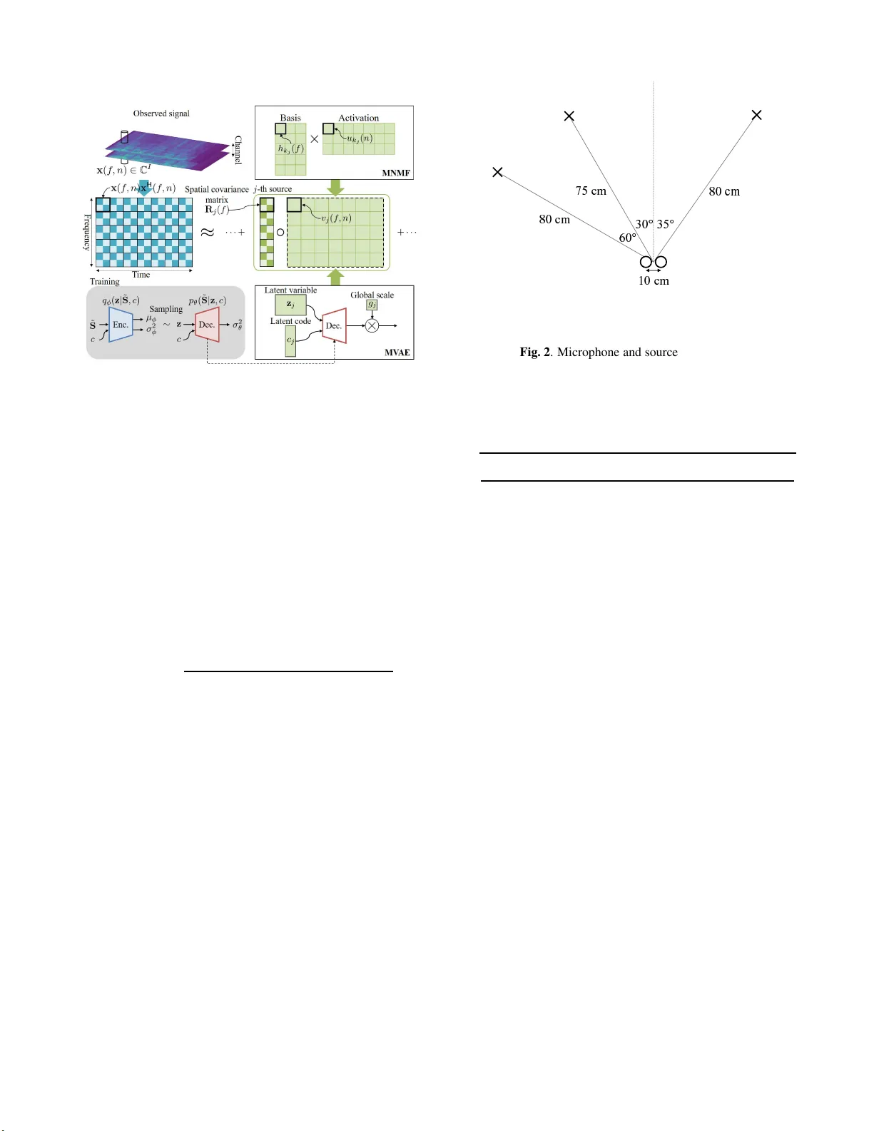
GENERALIZED MUL TICHANNEL V ARIA TIONAL A UT OENCODER FOR UNDERDETERMINED SOURCE SEP ARA TION Shogo Seki 1) , Hir okazu Kameoka 2) , Li Li 3) , T omoki T oda 4) , Kazuya T akeda 5) 1) Graduate School of Informati cs, Nagoya University , Japan 2) NTT Comm unication Science Laboratori es, Nippo n T elegraph and T elepho n e Corporatio n, Japan 3) Graduate School of Systems and Information E ngineering, Univ ersity of Tsukub a, Japan 4) Information T echnology Center , Nagoya University , Japan 5) Institutes o f Inn ovation for Future Society , Nagoya University , Japan ABSTRA CT This pa per deals with a multi channel audio source separation prob- lem under underdetermine d conditions. Multichannel Non-neg ativ e Matrix Factorization (MNMF) is one of powerful approache s, which adopts the NMF concep t for source power spectrogram modeling. This concept is also employed in Independen t Low-Rank Matrix Analysis (ILRMA), a special class of the MNMF f r amework for- mulated under determined conditions. While these methods work reasonably well for particular types of sound sources, one limitation is that they can fail t o work for sources with spectrograms that do not comply with the NMF model. T o address this limit ation, an ex- tension of ILRMA called the Multichannel V ariational Autoencode r (MV AE) method was recently proposed, where a Conditional V AE (CV AE) is used instead of the NMF model for source power spectro- gram modeling. This approach has shown to perform impressiv ely in determined source separation tasks thanks to the representation po wer of DNNs. While the original MV AE method was formu- lated under determined mixing conditions, this paper generalizes it so t hat it can also deal with underdetermined cases. W e call the pro- posed framew ork the Generalized MV AE ( G MV AE). The proposed method was ev aluated on a underdetermined source separation task of separating out three sources fr om two microphone inputs. Ex- perimental results revealed that the GMV AE method achie ved better performance than the MNMF method. Index T erms — Underdetermined source separation, Multichan- nel non-neg ativ e matrix factorization, Multichannel audoenc oder 1. INTRODUCTION Blind source separation (BS S) refers to a problem of separating out individ ual source signals from microphone array i nputs where the transfer functions between the sources and microphone s are un- kno wn. The fr equency-domain BS S approach allows the utilization of various models for the time-fr equency representations of source signals and/or arr ay responses. For example, Independent V ector Analysis (IV A) [1, 2] of fers a way of jointly solving frequenc y-wise source separation and permutation al i gnment under the assumption that the magnitudes of the frequency components originating f r om the same source are li kely to v ary coherently ov er time. Other appro aches in vo lve multichannel extensions of Non- negati v e Matrix Factorization (NMF) [3, 4, 5 , 6 , 7 ]. NMF was origi- nally applied to music transcription and monaural source separation tasks [8 , 9] where the idea i s to i nterpret the po wer spectrogram of a mixture signal and approximate it as the product of two non-ne gati ve matrices. This can be vie wed as approximating the power spectrum of a mixture signal observed at each time f rame by the sum of basis spectra scaled by time-varying magnitudes. Multichannel NMF (MNMF) is an extension of this approach to a multichannel case that al l o ws f or the use of spatial information. It can also be seen as an approach to frequency-do main BSS using spectral templates as a clue for jointly solving fr equenc y-wise source separation and permutation alignment. The original MNMF [3] was formulated under a general prob- lem setting where sources can outnumber microphones and a deter- mined version of MNMF was subsequently proposed i n [4]. While the determined version is applicable only to determined cases, it al- lo ws an implementation of a significantly faster algorithm t han the general version. The determined MNMF framewo rk was later called Independe nt Low-Rank Matrix Analysis ( I L RMA) [7]. The MNMF frame work including ILRMA is notable in t hat the optimization al- gorithm is guaranteed to con ver ge, ho we ver , one limit ation is that it can fail to work for sources wi th spectrograms that do not comply with the NMF model. T o address this limitation, a technique called the Multichan- nel V ariati onal Autoencoder (MV AE) method was recently proposed in [10]. I t is an extension of ILRMA in which a Conditional V AE (CV AE) [11] is used instead of the NMF model to esti mate the po wer spectrograms of the sources in a mixture. Specifically , MV AE al- lo ws the estimation of the separation matrices by employing a sin- gle CV AE, trained using the spectrograms of speech samples with speak er ID labels, as a generati ve model of the speech spectrograms of multiple speakers. This approach i s note worthy in that it can ex- ploit the benefits of the representation power of DNNs for source po wer spectrogram modeling and has shown t o outperform IL RMA on a determined source separation task. While t he original MV AE method was formulated under deter- mined mixing conditions, this paper generalizes it so that it can also deal wi th underdetermined cases. W e call the proposed framework Generalized MV AE (GMV AE) to distinguish it from the original de- termined version. 2. PROBLEM FORMULA TION W e consider a situation where J source signals are observed by I microphones. Let s j ( f , n ) and x i ( f , n ) be the Short-T ime Fourier T ransform (STFT) co efficient of the j -th source si gnal and the i -th observed signal, where f and n are the frequency and time indices, respecti vely . W e denote the vectors containing s 1 ( f , n ) , · · · , s J ( f , n ) and x 1 ( f , n ) , · · · , x I ( f , n ) by s ( f , n ) = [ s 1 ( f , n ) , · · · , s J ( f , n )] T ∈ C J , (1) x ( f , n ) = [ x 1 ( f , n ) , · · · , x I ( f , n )] T ∈ C I , (2) where ( · ) T denotes transpose. Now , we use a mixing system of the form x ( f , n ) = A ( f ) s ( f , n ) , (3) A ( f ) = [ a 1 ( f ) , · · · , a J ( f )] ∈ C I × J , (4) to describe the relationship between s ( f , n ) and x ( f , n ) where A ( f ) is called the mixing matrix. Here, we assume that s j ( f , n ) independently follows a zero- mean complex Gaussian distribution with variance v j ( f , n ) = E  | s j ( f , n ) | 2  s j ( f , n ) ∼ N C ( s j ( f , n ) | 0 , v j ( f , n )) . (5) Eq. (5) is called the Local Gaussian Model (LGM). When s j ( f , n ) and s j ′ ( f , n ) are independen t for j 6 = j ′ , s ( f , n ) follows s ( f , n ) ∼ N C ( s ( f , n ) | 0 , V ( f , n )) , (6) where V ( f , n ) is a diagonal matrix with diagonal entries v 1 ( f , n ) , · · · , v J ( f , n ) . From Eq. (3) and Eq. (6), x ( f , n ) is shown to follow x ( f , n ) ∼ N C ( x ( f , n ) | 0 , A ( f ) V ( f , n ) A H ( f )) , (7) where ( · ) H denotes conjugate tr anspose. Thus, the log-likelihood of the mixing matrices A = { A ( f ) } f and the va riances of source signals V = { v j ( f , n ) } f , n gi ven the observed mixture signals X = { x ( f , n ) } f , n is giv en by log p ( X |A , V ) c = − X f , n h tr ( x H ( f , n )( A ( f ) V ( f , n ) A H ( f )) − 1 x ( f , n )) + logdet ( A ( f ) V ( f , n ) A H ( f )) i , (8) where c = denotes equality up to constant terms. If there is no con- straint imposed on v j ( f , n ) , Eq. (8) will be split into frequenc y-wi se source separation problems. This indicates that there is a permu- tation ambiguity in the separated components for each fr equenc y since permutation of j does not affect the value of the log-likelihood. Thus, we usually need to perform permutation alignment after A is obtained. 3. RELA TED WORK 3.1. MNMF The spatial cov ariance of t he observed mixture signal A ( f ) V ( f , n ) A H ( f , n ) can be re wr i tten as the linear sum of the outer products of a j ( f ) multiplied by v j ( f , n ) : A ( f ) V ( f , n ) A H ( f ) = X j a j ( f ) v j ( f , n ) a H j ( f ) = X j v j ( f , n ) R j ( f ) , (9) where R j ( f ) represents the spatial cova riance of source j . As with IV A, MNMF makes it possible to jointly solve frequency-wise source separation and permutation alignment by imposing a con- straint on v j ( f , n ) . Specifically , v j ( f , n ) is modeled as the linear sum of K j spectral templates h j, 1 ( f ) , · · · , h j,K j ( f ) ≥ 0 scaled by time-v arying activ ati ons u j, 1 ( n ) , · · · , u j,K j ( n ) ≥ 0 : v j ( f , n ) = K j X k =1 h j,k ( f ) u j,k ( n ) . (10) It is also possible t o allo w all t he spectral templates to be shared by e very source and let the contribution of the k -th spectral template to source j be determined in a data-dri ven manner . Thus, v j ( f , n ) can also be expressed as v j ( f , n ) = K X k =1 b j,k h k ( f ) u k ( n ) , (11) where b j,k ∈ [0 , 1] is a continuous indicator va riable that satisfies P k b j,k = 1 . Here, b j,k can be interpreted as the expectation of a binary indicator v ariable that describes the index of the source to which the k -th template is assigned. The optimization algorithm of MNMF consists of iterativ ely up- dating the spatial cov ariance matrices R = { R j ( f ) } j,f , and the source models H 1 = { h j,k ( f ) } j,k,f , U 1 = { u j,k ( n ) } j,k,n or B = { b j,k } j,k , H 2 = { h k ( f ) } k,f , U 2 = { u k ( n ) } k,n . W e can deri ve up- date equations using the principle of the Majorization-Minimization (MM) algorithm. For the update of R , we can use the solution to Algebraic Ricatti equation R j ( f ) Ψ j ( f ) R j ( f ) = Ω j ( f ) , (12) where Ψ j ( f ) = X n v j ( f , n ) ˆ X − 1 ( f , n ) , (13) Ω j ( f ) = R j ( f ) X n v j ( f , n ) ˆ X − 1 ( f , n ) X ( f , n ) ˆ X − 1 ( f , n ) ! R j ( f ) . (14) Note that we have used X ( f , n ) and ˆ X ( f , n ) to represent X ( f , n ) = x ( f , n ) x H ( f , n ) , (15) ˆ X ( f , n ) = A j ( f ) V ( f , n ) A j ( f ) . (16) Performing R j ( f ) ←  R j ( f ) + R H j ( f )  / 2 and R j ( f ) ← R j ( f ) + ǫ I after solving Eq. (12) is empirically sho wn to help av oid computational instability . As in [5], update rules for H 1 and U 1 can be derived as h j,k ( f ) ← h j,k ( f ) × v u u t P n u j,k ( n ) tr ( ˆ X − 1 ( f , n ) X ( f , n ) ˆ X − 1 ( f , n ) R j ( f )) P n u j,k ( n ) tr ( ˆ X − 1 ( f , n ) R j ( f )) , (17) u j,k ( n ) ← u j,k ( n ) × v u u u t P f h j,k ( f ) tr ( ˆ X − 1 ( f , n ) X ( f , n ) ˆ X − 1 ( f , n ) R j ( f )) P f h j,k ( f ) tr ( ˆ X − 1 ( f , n ) R j ( f )) . (18) When v j ( f , n ) is giv en in the f orm of Eq. (11 ) , update rules for B , H 2 , and U 2 can be derived as b j,k ← b j,k × v u u u t P f , n h k ( f ) u k ( n ) tr ( ˆ X − 1 ( f , n ) X ( f , n ) ˆ X − 1 ( f , n ) R j ( f )) P f , n h k ( f ) u k ( n ) tr ( ˆ X − 1 ( f , n ) R j ( f )) , (19) h k ( f ) ← h k ( f ) × v u u u t P j,n b j,k u k ( n ) tr ( ˆ X − 1 ( f , n ) X ( f , n ) ˆ X − 1 ( f , n ) R j ( f )) P j,n b j,k u k ( n ) tr ( ˆ X − 1 ( f , n ) R j ( f )) , (20) u k ( n ) ← u k ( n ) × v u u u t P j,f b j,k h k ( f ) tr ( ˆ X − 1 ( f , n ) X ( f , n ) ˆ X − 1 ( f , n ) R j ( f )) P j,f b j,k h k ( f ) tr ( ˆ X − 1 ( f , n ) R j ( f )) . (21) T o ensure that B satisfies t he sum-to-one constraint, we normalize B after performing Eq. (19) by b j,k ← b j,k / P k b j,k and rescale H 2 and U 2 accordingly . 3.2. ILRMA ILRMA is a special class of MNMF designed to solve determined source separation problems. Unlike MNMF , which uses the mixing system (Eq. (3)), ILRMA uses a separation system of the form s ( f , n ) = W H ( f ) x ( f , n ) , (22) W ( f ) = [ w 1 ( f ) , · · · , w I ( f )] ∈ C I × J , (23) assuming the mixing matrix is inv erti ble. The in verse matrix W H ( f ) is called the separation matrix. F rom Eq. (6) and Eq. (22), x ( f , n ) is sho wn to follo w x ( f , n ) ∼ N C ( x ( f , n ) | 0 , ( W H ( f )) − 1 V ( f , n )( W ( f )) − 1 ) . (24) The log-likelihood of the separation matrices W = { W ( f ) } f and V given the observed signals X is giv en by log p ( X |W , V ) c = 2 N X f log | det W H ( f ) | − X f , n,j " log v j ( f , n ) + | w H j ( f ) x ( f , n ) | 2 v j ( f , n ) # , (25) where v j ( f , n ) i s modeled as Eq. (10) or Eq. (11) as with MNMF . As wi th MNMF , we can deriv e MM-based update equations for H 1 , U 1 or B , H 2 , U 2 . Since ILRMA is a natural extension of IV A, we can use a fast update rule called the Iterativ e Projection (IP) [12] for the separation matrices, originally dev eloped for IV A. 3.3. DNN Approach There has been some studies attempting to integrate deep neural net- works (DNNs) with the LGM-based multichannel source separation frame work [13]. [13] proposes an algorithm that consists of updat- ing v j ( f , n ) for each j via the f orward computation of a pretrained DNN. Here, each DNN is trained so that it produces a denoised ver- sion of the input spectra. Hence, v j ( f , n ) is forced to get close to the spectra of clean speech at each iterati on. Howe ver , updating v j ( f , n ) in this way does not guarantee an increase in the log-likelihood, which does not ensure the con vergence of the devised algorithm. 3.4. M V AE One li mitation of t he MNMF framewo rk including ILRMA is that since v j ( f , n ) is restricted to Eq. (10), it can fail to work for sources with spectrograms that do not actually follow this form. The MV AE method is an extension of ILRMA that replaces E q. (10) with a pre- trained CV AE. Let ˜ S = { s ( f , n ) } f , n be the complex spectrogram of a particular sound source. MV AE models the generati ve model of ˜ S using a Conditional V AE (C V AE) with an auxiliary input c . Here, we assume that c is represented as a one-hot vector , indicating the class of a source. Thus, the elements of c must sum to unity . For examp le, if we consider speaker identities as the source class, each element of c wi ll be associated wit h a differe nt speaker . The CV AE consists of an encode r network and a decoder net- work, w hich are assumed to be tr ained using labeled training ex- amples { ˜ S m , c m } M m =1 prior to separation. The encoder distribution q φ ( z | ˜ s , c ) is expressed as a Gaussian distribution: q φ ( z | ˜ S , c ) = Y k N ( z ( k ) | µ φ ( k ; ˜ S , σ 2 φ ( k ; ˜ S , c )) , (26) where z denotes a latent space v ariable and z ( k ) , µ φ ( k ; ˜ S ) , and σ 2 φ ( k ; ˜ S , c ) represent the k –th elements of z , µ φ ( ˜ S , c ) , and σ 2 φ ( ˜ S , c ) , respecti vely . The decoder distribution p θ ( ˜ S | z , c, g ) is expressed as a zero-mean complex Gaussian distribution (LGM): p θ ( ˜ S | z , c, g ) = Y f , n N C ( s ( f , n ) | 0 , v ( f , n )) , (27) v ( f , n ) = g · σ 2 θ ( f , n ; z , c ) , (28) where σ 2 θ ( f , n ; z , c ) r epresents the ( f , n ) –th elements of the decoder output σ 2 θ ( z , c ) and g i s the global scale of the generated spectro- gram. Both the encoder and decoder network parameters φ , θ are trained using the follo wing objectiv e fucntion J ( φ, θ ) = E ( ˜ S ,c ) ∼ p D ( ˜ S ,c ) h E z ∼ q ( z | ˜ S ,c ) [log p ( ˜ S | z , c )] − KL [ q ( z | ˜ S , c ) || p ( z )] i , (29) where E ( ˜ S ,c ) ∼ p D ( ˜ S ,c ) [ · ] denotes the sample mean over the training examp les and KL [ ·||· ] is the Kullback -Leibler dive rgence. The t rained decoder distri bution p θ ( ˜ S | z , c, g ) is considered as a universa l generativ e model that is capable of generating spectro- grams of all the sources inv olved in the training examples. MV AE employ s the decoder part of the CV AE as the source model v j ( f , n ) in Eq. (25) and treats the input z and c to the decoder as the model parameters to be estimated. The optimization algorithm of MV AE consists of updating the separation matrices using IP , the global scale and t he input to the pretrained decoder using backpropagation. The adv antage of the MV AE is that it can lev erage the strong representa- tion powe r of V AE f or source power spectrogram modeling. Fig. 1 . Illustration of Generalized MV AE 4. GENERALIZED MV AE While the MV AE method is applicable only to determined mixtures, we propose generalizing i t to so that it can also deal with underde- termined mixtures. As with the original MV AE method, we use the decoder network of the pretrained CV AE as the generativ e model of source po wer spectrograms. Fi g. 1 shows an illustration of GMV AE and MNMF with the source model giv en by E q. (10 ). Since the decoder distri bution is giv en in the same form as the LGM, we can use p θ ( ˜ S j | z j , c j , g j ) to dev elop the log-likelihood of the form Eq. (8). Hence, we can derive an iterativ e algorithm for estimating R , G = { g j } j , and Ψ = { z j , c j } j in the same way as the deri v ation of t he MM-based algorithm for MNMF . According to [14], we can show that L = − log p ( X |A , V ) c ≤ X j X f , n  tr ( X ( f , n ) P j ( f , n ) R − 1 j ( f , n ) P j ( f , n )) v j ( f , n ) + v j ( f , n ) tr ( K − 1 ( f , n ) R j ( f , n ))  , (3 0) where the equality holds when P j ( f , n ) = v j ( f , n ) R j ( f , n ) X j v j ( f , n ) R j ( f , n ) ! − 1 , (31) K ( f , n ) = X ( f , n ) . (32) Thus, we can use the right-hand side of this inequality as a majorizer of L where P = { P j ( f , n ) } j,f,n and K = { K ( f , n ) } f , n are aux- iliary variab les. An iterative algorithm that consists of minimizing this majorizer wit h respect to R , G , and Ψ and updating P and K at Eq. (31) and E q. (32) is guaranteed to conv erge to a st at i onary point of L . The optimal update of R is gi ven as t he solution to Eq. (12). Since the majorizer is split into source-wise terms, Ψ can be updated parallelly using backpropagation. Note that we must take account of the sum-to-one constraints when updating c j . This can be easily im- plemented by inserting an appropriately designed softmax l ayer that outputs c j c j = softmax ( d j ) , (33)                          Fig. 2 . Microphone and source positions and treating d j as the parameter to be estimated instead. The optimal update of G is obtained as g j ← g j × v u u u t P f , n σ 2 θ ( f , n ; z j , c j ) tr ( ˆ X − 1 ( f , n ) X ( f , n ) ˆ X − 1 ( f , n ) R j ( f )) P f , n σ 2 θ ( f , n ; z j , c j ) tr ( ˆ X − 1 ( f , n ) R j ( f )) . (34) The source separation algorithm of GMV AE i s summarized as fol- lo ws: 1. Train φ and θ using Eq. (29). 2. I nit i alize R , G , and Ψ = { z j , c j } . 3. I t erate the following steps for each j : (a) Up date R using Eq. (12), Eq. (13), and Eq. (14). (b) Update ψ j = { z j , c j } using backpropagation . (c) Up date g j using Eq. (34). 5. EXPERIMENT AL EV ALU A TIONS The proposed method was ev aluated on an underdetermined source separation task of separating out three sources from two microphone inputs. As the experimen tal data, we used speech samples of the V oice Con version Challenge (VCC) 2018 dataset [15 ] , which con- tains recordings of six female and six male US English speakers. Specifically , we used a set of the utterances of two female and two male speakers, ’SF1’, ’S F2’, ’ S M1’, and ’S M2’. In this experiment, speak er identities are considered as t he source class category: c is represented as a four-dimension al one-hot vector . 81 sentences and 35 sentences of each speaker were used for training and ev aluation, respecti vely . Fig. 2 sho ws the position of microphones and sources. ❞ and × show the microphones and sources, respective ly . 10 speech mixtures are generated for four speak er patterns: SF 1+SF2+SM2, SF1+SM1+SF2, SF1+SM1+SM2, and S M1+SF2+SM2. All the speech signals were resampled at 16 [kHz] and STFT analysis was conducted with 256 [ms] frame length and 128 [ms] hop length. W e designed the encoder and decoder networks of the CV AE as a three-layer fully-con volutiona l network with gated lin- ear units and a three-layer fully-decon volutional network with gated linear units as in [10 ]. The Adam [16] algorithm with learning rate SF1+SF2+SM2 SF1+SM1+SF2 SF1+SM1+SM2 SM1+SF2+SM2 0.0 1.0 2.0 3.0 4.0 SDR [dB] MNMF1 MVAE1 MNMF2 MVAE2 SF1+SF2+SM2 SF1+SM1+SF2 SF1+SM1+SM2 SM1+SF2+SM2 0.0 2.0 4.0 6.0 8.0 ISR [dB] MNMF1 MVAE1 MNMF2 MVAE2 SF1+SF2+SM2 SF1+SM1+SF2 SF1+SM1+SM2 SM1+SF2+SM2 0.0 1.0 2.0 3.0 4.0 5.0 6.0 SIR [dB] MNMF1 MVAE1 MNMF2 MVAE2 SF1+SF2+SM2 SF1+SM1+SF2 SF1+SM1+SM2 SM1+SF2+SM2 0.0 2.0 4.0 6.0 8.0 SAR [dB] MNMF1 MVAE1 MNMF2 MVAE2 Fig. 3 . A veraged separation performances for T 60 = 78 [ ms ] SF1+SF2+SM2 SF1+SM1+SF2 SF1+SM1+SM2 SM1+SF2+SM2 0.0 1.0 2.0 3.0 4.0 5.0 SDR [dB] MNMF1 MVAE1 MNMF2 MVAE2 SF1+SF2+SM2 SF1+SM1+SF2 SF1+SM1+SM2 SM1+SF2+SM2 0.0 2.0 4.0 6.0 8.0 10.0 ISR [dB] MNMF1 MVAE1 MNMF2 MVAE2 SF1+SF2+SM2 SF1+SM1+SF2 SF1+SM1+SM2 SM1+SF2+SM2 0.0 2.0 4.0 6.0 8.0 SIR [dB] MNMF1 MVAE1 MNMF2 MVAE2 SF1+SF2+SM2 SF1+SM1+SF2 SF1+SM1+SM2 SM1+SF2+SM2 0.0 2.0 4.0 6.0 8.0 SAR [dB] MNMF1 MVAE1 MNMF2 MVAE2 Fig. 4 . A veraged separation performances for T 60 = 351 [ ms ] 0.0002 was used to train the CV AE and the Stochastic Gradient De- scent (S GD) algorithm with learning rate 0.0005 was used to update the V AE source model Ψ . W e chose the MNMF algorithm with the source model given by E q. (10) or E q. (11) as baseline methods (MNMF1, MNMF2) for comparison. The separation algorithm was run for 300 iterations for the con ventional methods and 100 itera- tions for the proposed. The parameters of the proposed method were initialized using t he baseline method run for 200 iterations. There- fore, we tested the proposed method with two different initial set- tings (MV AE1, MV AE2). As the e v aluation metrics, the Signal-to- Distortion R atio (SDR), the source Image-to-Spatial distortion ra- tio (ISR), the Signal-to-Inference Ratio (SIR), and the S ignal-to- Artifact Ratio (SA R ) [17] between the reference signals and the sep- arated signals were calculated for each mixture and averag ed over 10 samples i n each speaker pattern. Separation performance was in vestigated with two different rev erberant conditions where the re- verberation times T 60 were set to 78 [ms] and 351 [ms], respecti vely . The separation performance under each rev erberant condition is sho wn i n Fig. 3 and 4. W e can see that the proposed method obtained better separation performance than the baseline methods. The results imply that the use of V AE source model has successfully contributed to improvin g the separation performance. 6. CONCLUSION This paper proposed the GMV AE method, which generalizes t he MV AE method so that i t can also be applied to multichannel source separation method under underdetermined conditions. Experimen- tal results revea led that the GMV AE method achiev ed better perfor- mance than the baseline method. 7. REFERENCES [1] T aesu Kim, T orbjørn El t oft, and T e-W on Lee, “Indep endent vector analysis: An extension of ica to multiv ariate compo- nents, ” in International Confer ence on Independen t Compo- nent Analysis and Signal Separa tion . S pringer , 2006, pp. 165– 172. [2] Atsuo Hi roe, “Solution of permutation problem in frequency domain ica, using multiv ariate probability density functions, ” in International Conferen ce on Independent Component Anal- ysis and Signal Separ ation . Springer, 2006, pp. 601–608. [3] Alex ey Ozerov and C ´ edric F ´ evotte, “Multichannel nonne gati ve matrix factorization in con voluti ve mixtures for audio source separation, ” IEEE T ransac tions on Audio, Speech, and Lan- guag e Processin g , vol. 18, no. 3, pp. 550–563 , 2010. [4] Hirokazu Kameoka, T akuya Y oshioka, Marik o Hamamura, Jonathan Le Roux, and Kunio Kashino, “Statistical model of speech signals based on composite autoregressi ve system with application to blind source separation, ” in International Confer ence on Latent V ariable Analysis and Signal S epara tion . Springer , 2010, pp. 245–253. [5] Hiroshi Sawada, Hirokazu Kameoka, Shoko Araki, and Naonori Ueda, “Multichann el extensions of non-ne gati ve ma- trix factorization wi th complex-v alued data, ” IEEE T ransac - tions on Au dio, Speec h, and Languag e Processing , vol. 21, no. 5, pp. 971–982, 2013. [6] Daichi Ki tamura, Nobutaka Ono, Hiroshi Sawada, Hirokazu Kameoka, and Hi r oshi S aruwatari, “Determined blind source separation unifying independent vector analysis and nonne ga- tiv e matrix factorization, ” IEEE/ACM T ransactions on Audio, Speec h and Languag e Processin g (T ASLP) , vol. 24, no. 9, pp. 1622–1 637, 2016. [7] Daichi Ki tamura, Nobutaka Ono, Hiroshi Sawada, Hirokazu Kameoka, and Hi r oshi S aruwatari, “Determined blind source separation with i ndepend ent low-rank matrix analysis, ” in Au- dio Sour ce Separation , pp. 125–15 5. S pringer , 2018. [8] Paris Smaragdis and Judith C Brown, “Non-n egati ve matrix factorization for polypho nic music transcription, ” in IE EE workshop on applications of signal pr ocessing to audio and acoustics . New Y ork, 2003, vol. 3, pp. 177–18 0. [9] C ´ edric F ´ evotte, N ancy Bertin, and Jean-Louis Durrieu, “Non- negati ve matri x factorization wit h the i takura-saito dive rgence: W ith application to music analysis, ” Neural computation , vol. 21, no. 3, pp. 793–830 , 2009. [10] Hirokazu Kameoka, Li Li, Shota Inoue, and Shoji Makino, “Semi-blind source separation with multichannel variational autoencod er , ” arXiv pr eprint arXiv:1808.0089 2 , 2018. [11] Diederik P Kingma, Shakir Mohamed, Danilo Jimenez Rezende, and Max W elling, “Semi-supervised learning with deep generati ve models, ” in Advances in Neural Information Pr ocessing Systems , 2014, pp. 3581–358 9. [12] Nob utaka Ono, “S t able and fast update rules for i ndepend ent vector analysis based on auxiliary function technique, ” in Ap- plications of Signal Proc essing to Audio and Acoustics (W AS- P AA), 2011 IEEE W orkshop on . IEEE, 2011, pp. 189–192 . [13] Aditya Arie Nugraha, Antoine Liutkus, and Emmanuel Vin - cent, “Multichannel audio source separation with deep neu- ral network s., ” IEEE/ACM T rans. Audio, Speech & L angua ge Pr ocessing , vol. 24, no. 9, pp. 1652–1664 , 2016. [14] Hirokazu Kameoka, Hiroshi Sawad a, and T akuya Higuchi, “General formulation of multichannel extensions of nmf va ri- ants, ” in Audio Sour ce Separ ation , pp. 95–124. Springer , 2018. [15] Jaime Lorenzo-Tru eba, Junich i Y amagishi, T omoki T oda, Daisuke Saito, Fernando V illavicencio, T omi Ki nnunen, and Zhenhua Li ng, “The voice con version challenge 2018: Pr o- moting de velopme nt of parallel and nonp arallel metho ds, ” arXiv pr eprint arXiv:1804.04262 , 2018. [16] Diederik P Kingma and Jimmy Lei Ba, “ Adam: Amethod for stochastic optimization, ” in Pr oceedings of the 3r d Interna- tional Confer ence on Learning Represe ntations (ICLR) , 2015. [17] Emmanu el V incent, R ´ emi Gribon val, and C ´ edric F ´ evotte, “Performance measurement in blind audio source separation, ” IEEE tr ansactions on audio, speec h, and lang uag e pr ocessing , vol. 14, no. 4, pp. 1462–1469, 2006.