Diffraction-Aware Sound Localization for a Non-Line-of-Sight Source

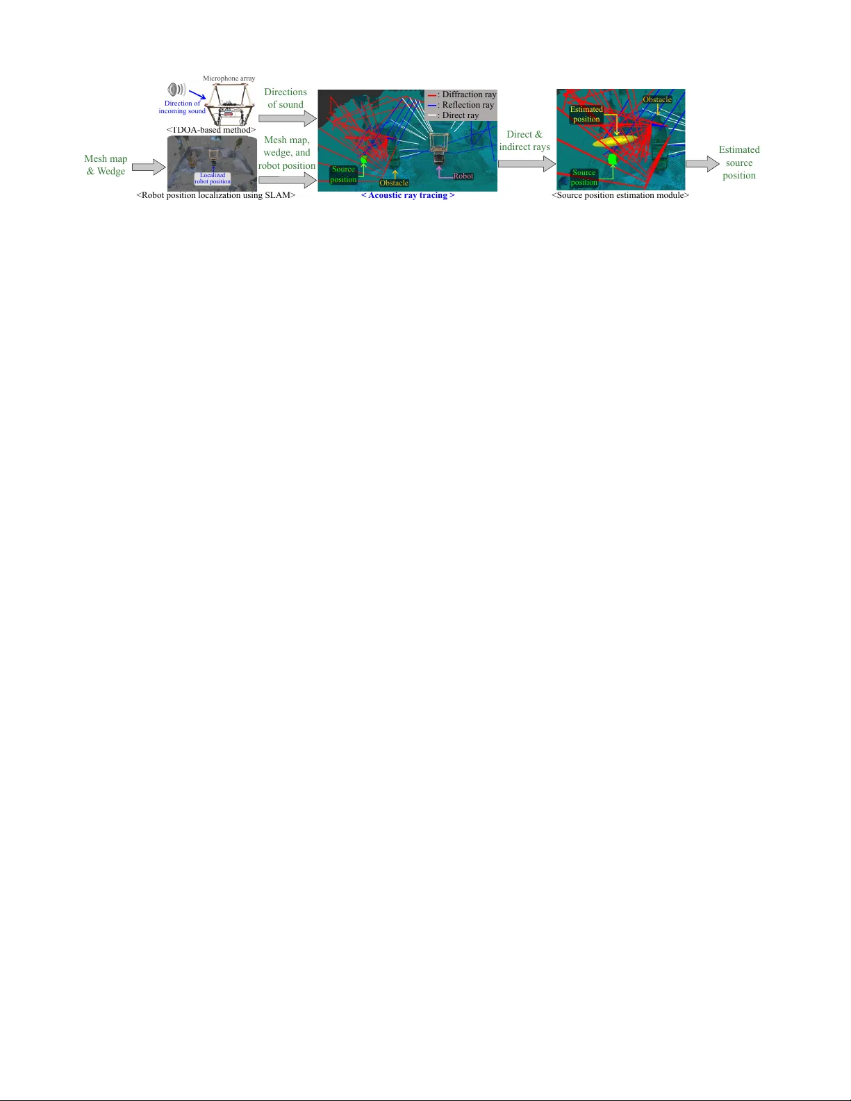
Diffraction-A war e Sound Localization f or a Non-Line-of-Sight Sour ce Inkyu An 1 , Doheon Lee 2 , Jung-woo Choi 3 , Dinesh Manocha 4 , and Sung-eui Y oon 5 Abstract — W e present a nov el sound localization algorithm for a non-line-of-sight (NLOS) sound source in indoor en vi- ronments. Our approach exploits the diffraction properties of sound waves as they bend around a barrier or an obstacle in the scene. W e combine a ray tracing based sound propagation algorithm with a Uniform Theory of Diffraction (UTD) model, which simulate bending effects by placing a virtual sound sour ce on a wedge in the en vironment. W e precompute the wedges of a reconstructed mesh of an indoor scene and use them to generate diffraction acoustic rays to localize the 3D position of the source. Our method identifies the conv ergence region of those generated acoustic rays as the estimated source position based on a particle filter . W e hav e evaluated our algorithm in multiple scenarios consisting of a static and dynamic NLOS sound source. In our tested cases, our approach can localize a source position with an average accuracy error , 0.7m, measured by the L2 distance between estimated and actual source locations in a 7m × 7m × 3m room. Furthermore, we observe 37% to 130% impro vement in accuracy over a state-of-the-art localization method that does not model diffraction effects, especially when a sound sour ce is not visible to the robot. I . I N T RO D U C T I O N As mobile robots are increasingly used for different ap- plications, there is considerable interest in developing new and improved methods for localization. The main goal is to compute the current location of the robot with respect to its en vironment. Localization is a fundamental capability required by an autonomous robot, as the current location is used to guide the future movement or actions. W e assume that a map of the environment is giv en and different sensors on the robot are used to estimate its position and orientation in the environment. Some of the commonly used sensors include GPS, CCD or depth cameras, acoustics, etc. In particular , there is considerable work on using acoustic sensors for localization, including sonar signal processing for underwater localization and microphone arrays for indoor and outdoor scenes. In particular , the recent use of smart microphones in commodity or IoT devices (e.g., Amazon Alexa) has triggered interest in better acoustic localization methods [1], [2], The acoustic sensors use the properties of sound wa ves to compute the source location. As the sound waves are emitted from a source, they transmit through the media and either reach the listener or microphone locations as direct paths, or after undergoing different wav e ef fects including reflections, 1 I. An, 2 D. Lee, and 5 S. Y oon (Corresponding author) are with the School of Computing, KAIST , Daejeon, South K orea; 3 J. Choi is with the School of Electrical Engineering, KAIST; 4 D. Manocha is with the Dept. of CS & ECE, Univ . of Maryland at College Park, USA; { inkyu.an, doheonlee, jwoo } @kaist.ac.kr, dmanocha@gmail.com, sungeui@kaist.edu Invisible area T raj ectory Starting point Goal Robot (listener) Obstacle Sound source (a) A Non-Line-of-Sight (NLOS) moving source scene around an obstacle. Our method can localize its position using acoustic sensors and our diffraction-a ware ray tracing. (b) Accuracy errors, measured as the L2 distance between the estimated and actual 3D locations of a sound source, for the dynamic source. Our method models dif fraction effects and improves the localization accuracy as compared to only modeling indirect reflections [8] Fig. 1. These figures show the testing en vironment (7m by 7m with 3m height) (a) and the accuracy error of our method with the dynamically moving sound source (b). The source mov es along the red trajectory , and the obstacle causes the in visible area for the dynamic source. Invisibility of the source occurs from 27s to 48s, where our method maintains a high accuracy , while the prior method deteriorates due to the diffraction: the av erage distance errors of our and the prior method are 0.95m and 1.83m. interference, dif fraction, scattering, etc. Some of the earliest work on sound source localization (SSL) makes use of the time difference of arriv al (TDO A) at the receiv er [3], [4]. These methods only exploit the direct sound and its direction at the receiv er, and do not take into account of reflections or other wav e ef fects. As a result, it does not provide sufficient accuracy for man y applications. Other techniques hav e been proposed to localize the position under different constraints or sensors [5], [6], [7], [8]. This includes modeling of higher order specular reflections [8] based on ray tracing and can model indirect sound effects. In many scenarios, the sound source is not directly in line of sight of the listener (i.e. NLOS) and is occluded by obstacles. In such cases, there may not be much contribution in terms of direct sound, and simple methods based on Point cloud <3D reconstruction> Mesh map Mesh map & W edge Fig. 2. This figure shows our precomputation phase. W e use SLAM to generate a point cloud of an indoor environment from the laser scanner and Kinect. The point cloud is used to construct the mesh map via 3D reconstruction techniques. W edges whose two neighboring triangles have angles larger than θ W and their edges are extracted from the mesh map to consider diffraction effects at runtime for sound localization. TDO A may not work well. W e need to model indirect sound ef fects and the most common methods are based on using ray-based geometric propagation paths. They assume the rectilinear propagation of sound wa ves and use ray tracing to compute higher order reflections. While they work well for high frequency sounds, but do not model many low-frequenc y phenomena like diffraction that is a type of scattering that occurs from obstacles whose size is of the same order of magnitude as the wav elength. In practice, diffraction is a fundamental mode of sound wa ve propagation and occurs frequently in building interior (e.g. source is behind an obstacle or hidden by w alls). These effects are more prominent for lo w-frequency sources, such as vo wel sounds in human speech, industrial machinery , ventilation, air-conditioned units. Main Results. W e present a nov el sound localization algorithm that takes into diffraction ef fects, especially from non-light-of-sight or occluded sources. Our approach is built on a ray tracing framework and models diffraction using the Uniform Theory of Diffraction (UTD) [9] along the wedges. During the precomputation phase, we use SLAM and recon- struct a 3D triangular mesh for an indoor en vironment. At runtime, we generate direct acoustic rays tow ards incoming sound directions as computed by TDOA. Once the acoustic ray hits the reconstructed mesh, we generate reflection rays. Furthermore, when acoustic rays pass close enough to the edges of mesh wedges according to our diffraction-criterion, we also generate diffraction acoustic rays to model non- visible paths to include an incident sound direction that can be actually traveled (Sec. III). Finally , we estimate the source position by performing generated acoustic rays using ray con vergence. W e have ev aluated our method in an indoor environment with three different scenarios, which include a stationary and a dynamically moving source along an obstacle that blocks the direct line-of-sight from the listener . In these cases, the diffracted acoustic wav es are used to localize the position. W e combine our diffraction method with reflection-aware SSL algorithm [8] and observe improvements from 1 . 22m to 0 . 7m on av erage and from 1 . 45m to 0 . 79m for the NLOS source. Our algorithm can localize a source generating the clapping sound within 1 . 38m as the worse error bound in a room of dimension 7 m × 7 m and 3m height. I I . R E L A T E D W O R K In this section, we gi ve a brief overvie w of prior work on sound source localization and sound propagation. Sound source localization (SSL). Ov er the past two decades, many approaches ha ve used time dif ference of arriv al (TDO A) to localize sound sources. Knapp et al. presented a good estimation of the time difference using a generalized correlation between a pair of microphone signals [3]. He et al. [4] suggested a deep neural network- based source localization algorithm in the azimuth direction for multiple sources. This approach focused on estimating an incoming direction of a sound and did not localize the actual position of the source. Recently , many techniques have been proposed to estimate the location of a sound source [5], [6], [7]. Sasaki et al. [5] and Su et al. [6] presented 3D sound source localization algorithms using a disk-shaped sound detector and a linear microphone array such as Kinect and PS3 Eye. Misra et al. [7] suggested a robust localization method in noisy en vironments using a drone. This approach requires the accumulation of steady acoustic signals at dif ferent positions, and thus cannot be applied to a transient sound ev ent or to stationary sound detectors. An et al. [8] presented a reflection-a ware sound source localization algorithm that used direct and reflected acoustic rays to estimate a 3D source position in indoor en vironments. Our approach is based on this work and takes into account diffraction effects to considerably improve the accuracy . Interactive sound propagation. There is considerable work in acoustics and physically-based modeling to dev elop fast and accurate sound simulators that can generate realistic sounds for computer-aided design and virtual en vironments. Geometry acoustic (GA) techniques have been widely uti- lized to simulate sound propagations ef ficiently using ray tracing techniques. Because ray tracing algorithms are based on the sound propagation model at high frequencies, low- frequency wa ve effects like diffraction are modeled sepa- rately . In addition, an estimation of the acoustic impulse response between the source and the listener was performed using Monte Carlo path tracing [10] or a hybrid combination of geometric and numeric methods techniques [11]. Exact methods to model diffraction are based on directly solving the acoustic wave equation using numeric methods like boundary or finite element methods [12], [13] or the BTM model [14] and its extension to higher order diffraction models [15]. Commonly used techniques to model diffraction with geometric acoustic methods are based on two models: the Uniform Theory of Diffraction (UTD) [16] and the Biot- T olstoy-Medwin (BTM) model [14]. The BTM model is an accurate diffraction formulation that computes an integral Mesh map & W edge Mesh map, wedge, and robot position Directions of sound < Acoustic ray tracing > Direct & indirect ray s Estimated source position Localized robot position Source position Obstacle Robot Obstacle Source position Estimated position Microphone array Direction of incoming sound : Dif fraction ray : Reflect ion ray : Direct ray Fig. 3. W e show run-time computations using acoustic ray tracing with diffraction rays for sound source localization. The diffraction-aware acoustic ray tracing is highlighted in blue and our main contribution in this paper. The source position estimation is performed by identifying ray conv ergence. of the dif fracted sound along the finite edges in the time domain [15], [13], [17]. In practice, the BTM model is more accurate, but is limited to non-interactiv e applications. The UTD model approximates an infinite wedge as a secondary source of diffracted sounds, which can be reflected and diffracted again before reaching the listener . UTD based approaches hav e been effecti ve for many real-time sound generation applications, especially in complex en vironments with occluding objects [18], [10]. Our approach is motiv ated by these real-time simulation and proposes a real-time source localization algorithm using UTD. I I I . D I FF R A C T I O N - A W A R E S S L W e present our diffraction-aw are SSL based on acoustic ray tracing, starting with giving its ov erview . A. Overview Precomputation. Given an indoor scene, we reconstruct a 3D model as part of the precomputation. W e use a Kinect and a laser scanner to capture a 3D point cloud representation of the indoor scene. As sho wn in Fig. 2, the point cloud capturing the indoor geometry information is generated by the SLAM module from raw depth data and an RGB-D stream collected by the laser scanner and Kinect. Next, we reconstruct a 3D mesh map via the generated point cloud. W e also extract wedges from the mesh that hav e angle, between two neighboring triangles, smaller than the threshold, Θ W . The reconstructed 3D mesh map and the wedges on it are used for our diffraction method at runtime. Runtime Algorithm. W e provide an ov erview of our runtime algorithm as it performs acoustic ray tracing and sound source localization in Fig. 3. Inputs to our runtime algorithm are the audio stream collected by the microphone array , the mesh map reconstructed in the precomputation, and the robot position localized by the SLAM algorithm. Our goal is find the 3D position of the sound source in the en vironment. Based on those inputs, we perform acoustic ray tracing supporting direct, reflection, and dif fraction effects by generating various acoustic rays (III-B). The source position is computed by estimating the conv ergence region of the acoustic rays (III-D). Our novel component, acoustic ray tracing with diffraction rays, is highlighted by the blue font in Fig. 3. B. Acoustic Ray T racing In this section, we explain how our acoustic ray tracing technique generates direct, reflection, and diffraction rays. At runtime, we first collect the directions of the incoming sound signals from the TDOA algorithm [19]. For each incoming direction, we generate a primary acoustic ray in the backward direction; as a result, we perform acoustic ray tracing in a backward manner . At this stage, we cannot determine whether the incoming signal is generated by one of the states: direct propagation, reflection, or dif fraction. W e can determine the actual states of these primary acous- tic rays while performing backward acoustic ray tracing. Nonetheless, we denote this primary ray as the direct acoustic ray since the primary ray is a direct ray from the listener’ s perspectiv e. W e represent a primary acoustic ray as r 0 n for the n -th incoming sound direction. Its superscript denotes the order of the acoustic path, where the 0-th order denotes the direct path from the listener . W e also generate a (backward) reflection ray once an acoustic ray intersects with the scene information under the assumption that the intersected material mainly consists of specular materials [8]. The main difference from the prior method [8] is that we use a mesh-based repre- sentation, while the prior method used a vox el-based octree representation for intersection tests. This mesh is computed during precomputation and we use the triangle normals to perform the reflections. As a result, for the n -th incoming sound direction, we recursi vely generate reflection rays with increasing orders, encoded by a ray path that is defined by R n = [ r 0 n , r 1 n , ... ] . The order of rays increases as we perform more reflection and diffraction. C. Handling Diffr action with Ray T racing W e now explain our algorithm to model the diffraction effects ef ficiently within acoustic ray tracing to localize the sound source. Since our goal is to achiev e fast performance in localizing the sound source, we use the formulation based on Uniform Theory of Diffraction (UTD) [16]. The incoming sounds collected by the microphone array consist of contrib utions from different ef fects in the en vironment, including reflections and diffractions. Edge diffraction occurs when an acoustic w av e hits the edge of a wedge. In the context of acoustic ray tracing, when an acoustic ray hits an edge of a wedge between two neighboring triangles, the diffracted signal propagates into all possible directions from that edge. The UTD model assumes that the point on the edge causing the diffraction effect is an imaginary source generating the spherical wav e [16]. In order to solve the problem of localizing the sound source, we simulate the process of backward ray tracing. Cone for UT D W edge Illuminated region Shadow region (a) Generating diffraction rays Shadow region Cone for UT D (b) Computing outgoing directions of diffraction rays. Fig. 4. This figure illustrates our acoustic ray tracing method for handling the diffraction ef fect. (a) Suppose that we have an acoustic ray r j − 1 n satisfying the diffraction condition, hitting or passing near the edge of a wedge. W e then generate N d diffraction rays cov ering the possible incoming directions (especially , in the shadow region) of rays that cause the diffraction. (b) An outgoing unit vector , ˆ d ( j , p ) n , of a p -th diffraction ray is computed on local coordinates ( ˆ e x , ˆ e y , ˆ e z ), and used after the transformation to the en vironment in runtime, where ˆ e z fits on the edge of the wedge and ˆ e x is set half-way between two triangles of the wedge. Suppose that an n -th incoming sound direction denoted by the ray r j − 1 n is generated by the diffraction effect at an edge. In an ideal case, the incoming ray will hit the edge of a wedge and generate the diffraction acoustic ray r j n , as shown in Fig. 4a; in the figure of (a), r ( j , · ) n is shown. It is important to note that there can be an infinite number of incident rays generating diffractions at the edge. Unfortunately , it is not easy to link the incident direction exactly to the edge generating the diffraction. Therefore, we generate a set of N d different diffraction rays in a backward manner that cov ers the possible incident directions to the edge based on the UTD model. This set is generated based on an assumption that one of those generated rays might ha ve the actual incident direction causing the diffraction. When there are sufficient acoustic rays, including the primary , reflection, and diffraction rays, it is highly likely that those rays will pass through or near to the sound source location; we choose a proper value of N d by analyzing diffraction rays (Sec. IV). This explanation begins with the ideal case, where the acoustic ray r j − 1 n hits the edge of a wedge. Because our algorithm works on the real en vironment containing various types of errors from sensor noises and resolution errors from the TDOA method, it is rare that an acoustic ray intersects an edge exactly . In order to support various cases that arise in real environ- ments, we propose using the notion of diffraction-condition between a ray and a wedge. The diffraction-condition simply measures how close the ray r j − 1 n passes to an edge of the wedge. Specifically , we define the dif fractability v d according to the angle θ D between the acoustic ray and its ideally generated ray for the diffraction with the wedge: i.e. v d = cos ( θ D ) , where the cos function is used to normalize the angle θ D (Fig. 5). Giv en an acoustic ray r j − 1 n , we define its ideally generated ray r 0 j − 1 n as the projected ray of r j − 1 n on the edge of the wedge where the end point m d of r 0 j − 1 n is on that edge (refer to the geometric illustration on Fig. 5). The point m d is located at the position closest to the point m j − 1 n of the input ray r j − 1 n ; due to the page limit, we do not sho w its detailed deri vation, b ut it can be defined based on our high- lev el description. If the diffractabilty v d is larger than a threshold value, e.g., 0 . 95 in our tests, our algorithm determines that the acoustic ray is generated from the diffraction at the wedge, and we thus generate the secondary , diffraction ray at the wedge in the backward manner . W e now present how to generate the dif fraction rays when the acoustic ray satisfies the diffraction-condition. The diffraction rays are generated along the surface of the cone (Fig. 4a) because the UTD model is based on the principle of Fermat [9]: the ray follo ws the shortest path from the source to the listener . The surface of the cone for the UTD model contains every set of the shortest paths. When the acoustic ray r j − 1 n satisfies the diffraction-condition, we compute outgoing directions for those diffraction rays. Those directions are the unit vectors generated on that cone and can be computed on a local domain as shown in Fig. 4b: ˆ d ( j , p ) n =   cos ( θ w / 2 + p · θ o f f ) sin θ d sin ( θ w / 2 + p · θ o f f ) sin θ d − cos θ d   , (1) where ˆ d ( j , p ) n denotes the outgoing unit vector of a p -th diffraction ray among N d different dif fraction rays, θ w is the angle between two triangles of the wedge, θ d is the angle of the cone that is same as the angle between the outgoing diffraction rays and the edge on the wedge, and θ o f f is the offset angle between two sequential diffraction rays, i.e. ˆ d ( j , p ) n and ˆ d ( j , p + 1 ) n , on the bottom circle of the cone. Giv en a hit point m d by an acoustic ray r j − 1 n on the wedge, we transform the outgoing directions in the local space to the world space by aligning their coordinates ( ˆ e x , ˆ e y , ˆ e z ). Based on those transformed outgoing directions, we then compute the outgoing diffraction rays, ¯ r ( j ) n = { r ( j , 1 ) n , ..., r ( j , N d ) n } , start- ing from the hit point m d . In order to accelerate the process, we only generate the diffraction rays in the shadow region, which is defined by the wedge; the rest of the shadow re gion is called the illuminated region. W e use this process because covering only the Initial ray : Ideally generated ray : Microphone array W edge Material 1 Fig. 5. This figure shows the diffraction condition. When a ray r j − 1 n passes close to an edge of a wedge, we consider the ray to be generated by the edge diffraction. W e measure the angle θ D between the ray and its ideal generated ray that hits the edge exactly , for checking our diffraction condition. shadow region b ut not the illuminated region generates minor errors for a simulation of the sound propagation [18]. Giv en the new diffraction rays, we apply our algorithm recursiv ely and generate another order of reflection and diffraction rays. Gi ven the n -th incoming direction signal, we generate acoustic rays, including direct, reflection, and diffraction rays and maintain the ray paths R n in a tree data structure. The root of this tree represents the direct acoustic ray , starting from the microphones. The depth of the tree denotes the order of its associated ray . Note that we generate one child and N d children for handling reflection and diffraction ef fects, respectiv ely . D. Estimating the Sour ce P osition W e explain our method used to localize the sound source position using acoustic rays. Our estimation is based on Monte-Carlo localization (MCL), also known as the particle filter [8]. Our estimation process assumes that there is a single sound source in the environment, which causes a high probability that all those acoustic ray paths pass near that source; Handling multiple targets using a particle filter has been also studied [20]. In other words, the acoustic rays con verge in a re gion located close to the source, and our estimation aims to identify such a con vergence region out of all the generated rays. The MCL approach generates initial particles in the space as an approximation to the source locations. It allocates higher weights to particles that are closer to acoustic rays and re-samples the particles to get more particles in re- gions with higher weights [8]. Specifically , we adopt the generalized v ariance, which is a one-dimensional measure for multi-dimensional scatter data, to see whether particles hav e conv erged. When the generalized variance is less than a threshold (e.g., σ c = 0 . 5), we treat that a sound occurs and the mean position of those particles as the estimated sound source position. I V . R E S U LT S A N D D I S C U S S I O N In this section, we describe our setup consisting of a robot with microphones and testing en vironments, and highlight the performance of our approach. The hardware platform is based on T urtlebot2 with a 2D laser scanner , Kinect, a computer with an Intel i7 process, and a microphone array , which is an embedded system for streaming multi- channel audios [21], consisting of eight microphones. For all the computations, we use a single core, and perform our estimation every 200ms, supporting five dif ferent estimations in one second. Benchmarks. W e hav e ev aluated our method in indoor en vironments containing a box-shaped object that blocks direct paths from the sound to the listener . W e use two scenarios: a stationary sound source and a moving source. As shown in Fig. 6, we place an obstacle between the robot and the stationary sound source, such that the source is not in the direct line-of-sight of the robot (i.e. NLOS source). W e use another testing en vironment with a source moving along the red trajectory , as shown in Fig. 1a. These two scenarios are tested on the same room that size is 7 m × 7 m and 3m height. During the precomputation phase, we perform SLAM and reconstruct a mesh of the testing en vironment. W e ensure that the resulting mesh has no holes using the MeshLab package. Stationary sound source with an obstacle. W e ev aluate the accuracy by computing the L2 distance errors between the positions estimated by our method and the ground-truth positions. W e use two types of sound signals: the clapping sound and male speech, where male speech has more low- frequency components than the clapping sound (dominant frequency range of the clapping sound: 2k ∼ 2.5kHz, and of male speech: 0.1k ∼ 0.7kHz). W e compare the accuracy of our approach with that of Reflection-A ware SSL (RA-SSL) [8], which models direct sound and indirect reflections, but no diffraction. For the stationary source producing clapping sound (Fig. 7a), the av erage distance errors of the RA-SSL and our method are 1 . 4m and 0 . 6m, respectiv ely . There are configurations of the sound source that are not visible to the microphone (NLOS). In this case, we observe 130% accuracy by modeling these diffraction rays. Fig. 7b sho ws the localization accuracy for the male speech signal, which has more low-frequency components. The measured distance errors are, on av erage, 1 . 12m for RA- Obstacle Robot 3 m Sound source Fig. 6. The e valuation environment for the static sound source. Direct paths from the sound source to the listener are blocked by the obstacle. W e use our diffraction-based algorithm for localization. (a) Stationary source (clapping). (b) Stationary source (male speech). Fig. 7. These graphs compare the localization distance errors of our method with the prior, reflection-aware SSL method [8] with the clapping sound source (a) and male speech signal source (b); green regions indicate no sound in that period. The av erage distance errors of RA-SSL and our method are 1.4m and 0.6m in (a), and 1.12m and 0.82m in (b), respectiv ely . The use of diffraction considerably reduces the localizatoin errors. SSL and 0 . 82m for our approach. While we also observe meaningful improv ement, it is less than we see with the clapping sound. Our method supports diffraction, b ut dif- fuse reflection is not yet supported. Given the man y low- frequency components of male speech, we observe that it is important to support diffuse reflection in addition to diffraction. Nonetheless, by modeling dif fraction for the male speech, we observe meaningful improv ement (37% on av erage) in localization accuracy . Moving sound source around an obstacle. W e also ev aluated our algorithm on a more challenging en vironment that contains a sound source (clapping sound) moving along the red trajectory shown in Fig 1a. Its accuracy graphs are presented in Fig. 1b; the a verage distance errors of the RA- SSL and ours are 1 . 15m and 0 . 7m, respectiv ely , indicating a 64% improvement in accuracy using our localization algorithm. It is interesting that, when the dynamic source is in the area corresponding to these time values (27s ∼ 48s), which are NLOS with respect to the robot, the av erage distance errors of the RA-SSL and our method are 1 . 83m and 0 . 95m, respecti vely , indicating a 92% improvement. This clearly demonstrates the benefits of our method in terms of localization. Overall, we achieved 130%, 37%, and 64% improvement, resulting in 77% average improv ement, on the stationary source with a clapping sound, the stationary source with male speech, and the dynamic source, respectiv ely , compared with the prior method RA-SSL [8]. The summary of the accuracy of our method compared with RA-SSL is in T able I. Analysis of diffraction rays. By modeling the diffraction effects, we increase the number of generated rays, resulting T ABLE I S U MM A RY O F T H E A CC U R AC Y O F T H E D I FF ER E N T M E TH O D S ( ∗ : O N L Y N L OS S O U RC E ) Scenario Stationary ∗ Stationary ∗ Dynamic Dynamic ∗ Sound Clapping Male voice Clapping Clapping RA-SSL 1.4m 1.12m 1.15m 1.83m Ours 0.6m (130%) 0.82m(37%) 0.7m(64%) 0.95m(92%) in a computational o verhead. As a result, we measure the av erage accuracy error and computation time as a function of N d the number of diffraction ray for simulating each edge dif fraction. As sho wn in Fig. 8, the average accuracy error gradually decreases, but we found that when N d is in a range of 2 to 5, the accuracy is rather saturated. Since we can accommodate to use up to N d = 5 given our runtime computation budget (0.2 s), we use N d = 5 across all the experiments. In this case, the av erage numbers of direct, reflection, and dif fraction rays are 18, 26, and 184, respectiv ely , in the case of the static source with clapping sound. Also, the av erage running times for acoustic ray tracing and particle filter are 0.09 ms and 72 ms ; our un- optimized particle filter uses 100 particles and computes weights of them against all the other rays. When we are done on estimating the location within the time budget, we let our process to be in the idle state. V . C O N C L U S I O N S & F U T U R E W O R K W e ha ve presented a novel diffraction-aw are source local- ization algorithm. Our approach can be used for localizing a NLOS source and models the diffraction ef fects using the uniform theory of diffraction. W e have combined our method with indirect reflections and ha ve tested our method in various scenarios with static and moving sound sources with different sound signals. While we hav e demonstrated benefits of our approach, it some limitations. The UTD model is an approximate model and mainly designed for infinite wedges. As a result, its accu- racy may v ary in different environment. W e observed lo wer accuracy for low-frequency sounds (male voice), mainly due to the diffuse effect. Our implemented approach is limited to a single sound source in the en vironment and does not model all the scattering effects. As part of future work, we would like to address these problems. Fig. 8. This figure sho ws the av erage accuracy error and computation time for our method on an Intel i7 processor 6700, as a function of N d the number of diffraction rays generated for simulating the edge diffraction. R E F E R E N C E S [1] Craig C Douglas and Robert A Lodder, “Human identification and localization by robots in collaborative en vironments”, Procedia Computer Science , vol. 108, pp. 1602–1611, 2017. [2] Muhammad Imran, Akhtar Hussain, Nasir M Qazi, and Muhammad Sadiq, “ A methodology for sound source localization and tracking: Dev elopment of 3d microphone array for near-field and far -field applications”, in Applied Sciences and T echnolo gy (IBCAST), 2016 13th International Bhurban Conference on . IEEE, 2016, pp. 586–591. [3] C. Knapp and G. Carter, “The generalized correlation method for estimation of time delay”, IEEE T rans. Acoust., Speech, Signal Pr ocess. , vol. 24, no. 4, pp. 320–327. [4] Petr Motlicek W eipeng He and Jean-Marc Odobez, “Deep neural networks for multiple speaker detection and localization”, in ICRA , 2018. [5] Y . Sasaki, R. T anabe, and H. T akemura, “Probabilistic 3d sound source mapping using moving microphone array”, in IROS , 2016. [6] D. Su, T . V idal-Calleja, and J. V . Miro, “T owards real-time 3d sound sources mapping with linear microphone arrays”, in ICRA , 2017. [7] Pragyan Mohapatra Prasant Misra, A. Anil Kumar and Balamuralidhar P ., “Droneears: Robust acoustic sound localization with aerial drones”, in ICRA , 2018. [8] Inkyu An, Myungbae Son, Dinesh Manocha, and Sung-eui Y oon, “Reflection-aware sound source localization”, in ICRA , 2018. [9] Joseph B Keller , “Geometrical theory of diffraction”, JOSA , vol. 52, no. 2, pp. 116–130, 1962. [10] Carl Schissler , Ravish Mehra, and Dinesh Manocha, “High-order diffraction and diffuse reflections for interactive sound propagation in large environments”, ACM Tr ansactions on Graphics (TOG) , vol. 33, no. 4, pp. 39, 2014. [11] Hengchin Y eh, Ravish Mehra, Zhimin Ren, Lakulish Antani, Dinesh Manocha, and Ming Lin, “W ave-ray coupling for interactive sound propagation in large complex scenes”, ACM Tr ansactions on Graphics (TOG) , vol. 32, no. 6, pp. 165, 2013. [12] B T eng and R Eatock T aylor , “New higher-order boundary element methods for wav e diffraction/radiation”, Applied Ocean Researc h , vol. 17, no. 2, pp. 71–77, 1995. [13] Sara R Martin, U Peter Svensson, Jan Slechta, and Julius O Smith, “ A hybrid method combining the edge source integral equation and the boundary element method for scattering problems”, in Pr oceedings of Meetings on Acoustics 171ASA . ASA, 2016, vol. 26, p. 015001. [14] U Peter Svensson, Roger I Fred, and John V anderkooy , “ An analytic secondary source model of edge diffraction impulse responses”, The Journal of the Acoustical Society of America , vol. 106, no. 5, pp. 2331–2344, 1999. [15] Andreas Asheim and U Peter Svensson, “ An integral equation formulation for the dif fraction from conv ex plates and polyhedra”, The Journal of the Acoustical Society of America , vol. 133, no. 6, pp. 3681–3691, 2013. [16] Robert G Kouyoumjian and Prabhakar H Pathak, “ A uniform geo- metrical theory of diffraction for an edge in a perfectly conducting surface”, November , vol. 88, pp. 1448–1461, 1974. [17] Lakulish Antani, Anish Chandak, Micah T aylor , and Dinesh Manocha, “Efficient finite-edge diffraction using conservati ve from-region visi- bility”, Applied Acoustics , vol. 73, no. 3, pp. 218–233, 2012. [18] Nicolas Tsingos, Thomas Funkhouser , Addy Ngan, and Ingrid Carl- bom, “Modeling acoustics in virtual environments using the uniform theory of diffraction”, in Pr oceedings of the 28th annual conference on Computer graphics and interactive techniques . ACM, 2001, pp. 545–552. [19] J.-M. V alin, F . Michaud, and J. Rouat, “Robust localization and tracking of simultaneous moving sound sources using beamforming and particle filtering”, Robot. Auton. Syst. , vol. 55, no. 3. [20] K. Okuma, A. T aleghani, N. d. Freitas, J. J. Little, and D. G. Lowe, “ A boosted particle filter: Multitarget detection and tracking”, in ECCV , 2004. [21] S. Briere, J.-M. V alin, F . Michaud, and D. L ´ etourneau, “Embedded auditory system for small mobile robots”, in ICRA , 2008.