Online Nonlinear Estimation via Iterative L2-Space Projections: Reproducing Kernel of Subspace

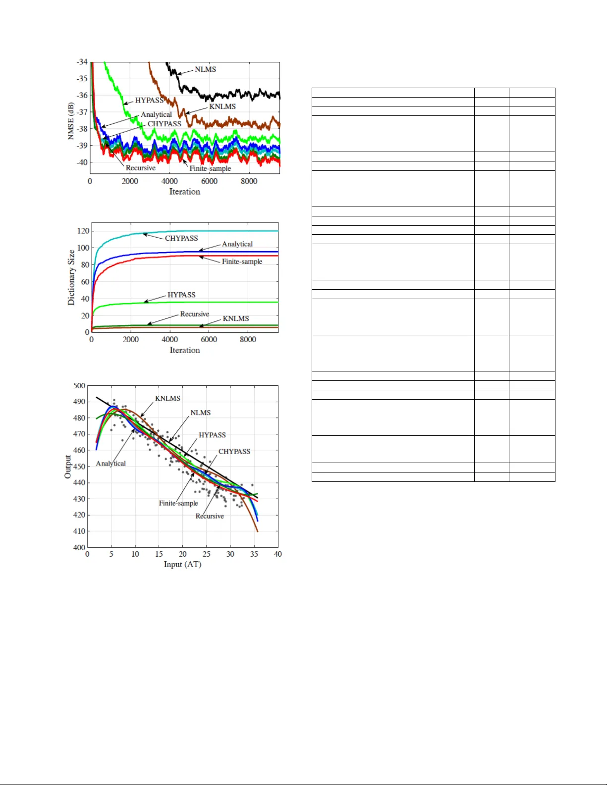
1 Online Nonlinear Estimation via Iterati v e L 2 -Space Projections: Reproducing K ernel of Subspace Motoya Ohnishi, Student Member , IEEE , and Masahiro Y uka wa, Member , IEEE Abstract — W e propose a novel online learning paradigm for nonlinear -function estimation tasks based on the iterative pro- jections in the L 2 space with probability measur e reflecting the stochastic property of input signals. The proposed learning algorithm exploits the reproducing kernel of the so-called dic- tionary subspace, based on the fact that any finite-dimensional space of functions has a repr oducing kernel characterized by the Gram matrix. The L 2 -space geometry pr ovides the best decorrelation property in principle. The proposed learning paradigm is significantly different fr om the con ventional ker nel- based learning paradigm in two senses: (i) the whole space is not a reproducing kernel Hilbert space and (ii) the minimum mean squared error estimator gives the best approximation of the desired nonlinear function in the dictionary subspace. It preser ves efficiency in computing the inner product as well as in updating the Gram matrix when the dictionary grows. Monotone approximation, asymptotic optimality , and con vergence of the proposed algorithm are analyzed based on the variable-metric version of adaptive projected subgradient method. Numerical examples show the efficacy of the proposed algorithm for real data over a variety of methods including the extended Kalman filter and many batch machine-lear ning methods such as the multilayer perceptron. Index T erms — online lear ning, metric projection, kernel adap- tive filter , L 2 space, recursive least squares I . I N T RO D U C T I O N A. Bac kgr ound Metric is a dominant factor in controlling con ver gence behaviors of online learning algorithms, as witnessed by the extensi ve studies on adaptiv e filtering [2]–[8] as well as the recent advances in stochastic optimization [9]–[12] (see also [13, Chapter 3] for a related idea called space dilation for accelerating the con ver gence of the subgradient method for minimization of nondifferentiable functions). Metric projec- tion has been used e xtensiv ely in adapti ve/online learning algorithms [14]–[21] (see also the tutorial paper [22]). The main subject of the present study is the metric of online learning algorithms for nonlinear -function estimation tasks. Kernel adaptiv e filtering is a po werful approach to the non- linear estimation tasks [23]–[42], being an adaptive extension of the kernel ridge regression [43], [44] or Gaussian process This work was partially presented at EUSIPCO 2017 [1]. This work was supported by JSPS Grants-in-Aid (15K06081, 15K13986, 15H02757) and Scandinavia-Japan Sasakawa Foundation. The real GPS data used in the numerical experiment is recorded by Isaac Skog at KTH Royal Institute of T echnology . M. Ohnishi is with the Department of Electronics and Electrical Engineer- ing, Keio University , Japan (e-mail: ohnishi@ykw .elec.keio.ac.jp). M. Y ukawa is with the Department of Electronics and Electrical Engineer- ing, Keio University , Japan (email: yukawa@elec.keio.ac.jp), and with the Center for Advanced Intelligence Project, RIKEN, Japan. [45]. Projection-based k ernel adapti ve filtering algorithms hav e been studied mainly by casting the nonlinear estimation as a minimization problem either (i) in the Euclidean space of coefficient vectors [30], or (ii) in the reproducing kernel Hilbert space (RKHS) [29], [31], [34], [35]. The two types of formulation induce two dif ferent geometries. The latter type is referred to as the functional approach, and its geometry in the dictionary subspace (i.e., the subspace spanned by the dictionary) can be expressed in the Euclidean space equiv a- lently with a metric characterized by the kernel matrix [35]. The functional approach tends to exhibit better con ver gence behaviors (see, e.g., [34], [35], [46]) than the former approach. This has been supported theoretically in [47]. Specifically , provided that the dictionary can be considered as a set of realizations of the input vectors, the autocorrelation matrix can be approximated by a squared kernel matrix essentially , which indicates that its eigen value spread for the functional approach is reduced to a square root compared to the former approach in principle. The con ventional kernel adaptive filtering methods employ a single kernel, thereby working efficiently only when all the three conditions are satisfied: (i) the target nonlinear function is sufficiently simple , (ii) its scale is kno wn prior to adaptation so that one can design a Gaussian kernel with appropriate scale, and (iii) the scale is time-inv ariant. Multikernel adaptiv e filtering [46], [48]–[50] is an efficient solution to the case in which some of the above conditions are violated, such as the case of multi-component/partially- linear functions (see [46]). A remarkable feature of multikernel adaptiv e filtering is that finding a well-fitting kernel and ob- taining a compact representation (i.e., dictionary sparsification and parameter estimation) are simultaneously achieved within a con vex analytic frame work. The existing functional approach for multikernel adaptiv e filtering is called the Cartesian hyper- plane projection along affine subspace (CHYP ASS) algorithm [46], formulated in the Cartesian product of the RKHSs associated with the multiple kernels employed. Here, CHY - P ASS is a multikernel extension of the hyperplane projection along affine subspace (HYP ASS) algorithm [34], [51], which is an ef ficient functional approach derived by formulating the normalized least mean square (NLMS) algorithm in the functional subspace. The decorrelation property of CHYP ASS is howe ver suboptimal since it counts no correlations among different kernels. B. Motivation and Contributions Suppose that the input (sample) is a real random vector . Our first primitiv e question is the following: what metric induces 2 the best geometry having a perfect decorrelation pr operty for online nonlinear-function estimation over a (possibly e xpand- ing) finite-dimensional subspace in general? An immediate answer to this question is the L 2 space (the set of square- integrable functions) under the probability measure determined by the probability density function of the input vector (see Sections II-A and III-A). Henceforth, we simply call it the L 2 space. In addition to its nice geometric property , the L 2 space is sufficiently large to accomodate the subspace ev en if it expands as time goes by (see Section II-A). The L 2 space, howe ver , is not an RKHS because the function value at some specific point is not well-defined due to the presence of equiv alence class. No w arises the central question penetrating this paper . Should the learning space be an RKHS to achieve efficient online nonlinear estimation? In this paper , we propose an efficient online nonlinear- function learning paradigm based on iterative projections in the L 2 space. In the proposed learning paradigm, the mini- mum mean squared error (MMSE) estimator giv es the best approximation (in the L 2 -metric sense) of the target nonlinear function in the dictionary subspace (Proposition 1 in Section III-A). W e highlight the fact that the HYP ASS algorithm implicitly e xploits the reproducing kernel of the dictionary subspace for updating the estimates (see Section II-D). W e then sho w the way of constructing the reproducing kernel of a finite-dimensional subspace in terms of the Gram matrix of its basis (Proposition 2 in Section III-A). W e can thus extend the strategy of HYP ASS to any space (which possibly has no reproducing kernel) in principle as long as the Gram matrix is computable at least approximately . The key idea is the following: (i) we make the function values well-defined in the dictionary subspace by not con- sidering the equiv alence class, and (ii) we then define the reproducing kernel of the dictionary subspace of the L 2 space. For implementing the proposed method efficiently , we present three practical examples of computing the Gram matrix. 1) When the basis contains multiple Gaussian functions with different centers and scale parameters, the inner product can analytically be computed by assuming that the input vec- tor obeys the normal distribution, or perhaps the improper constant distribution in analogy with a conjugate prior and a noninformative prior in Bayesian statistics. 2) The Gram matrix can be approximated with the atoms of the dictionary under a certain condition. 3) The Gram matrix can recursi vely be updated by using the matrix in version lemma for rank- 2 update. W e show that the approximate linear dependency (ALD) condition [25] ensures a lower bound of the amount of the MMSE reduction due to the newly entering dictionary- element, keeping in mind the link between ALD and the co- herence condition [30] (which we shall use for computational efficienc y). See Lemma 1 and Proposition 4 in Section III- C. The computational complexity of the proposed algorithm has the same order as that of the Euclidean approach when the selectiv e-update strategy is employed (see Section III- D). Monotone approximation, asymptotic optimization, and con vergence of the proposed algorithm are proved for the full-updating case within the framework of the variable-metric T ABLE I C O M PA R I S O N S O F T H E P R O J E C T I O N - B A S E D M E T H O D S T O B A Y E S I A N A N D S T O C H A S T I C G R A D I E N T D E S C E N T A P P RO AC H E S Algorithm Con ver gence T racking Complexity V ariance speed information Online GPs very fast slow high yes KRLS-T fast fast high yes NORMA moderate moderate low unin vestigated Projection fast very fast low unin vestigated adaptiv e projected subgradient method (APSM) [4], [52] (The- orem 2 in Section IV). Numerical examples show that (i) the proposed algorithm enjoys a better decorrelation property than CHYP ASS [46] and the multikernel NLMS (MKNLMS) algorithm [48], and (ii) it outperforms, under the use of the selectiv e-update strategy , the extended Kalman filter (EKF) for real data as well as 13 (out of 15 ) batch learning methods that hav e been compared in the literature [53], [54]. C. Relations to Bayesian and Stochastic Gradient Descent Appr oaches The projection-based methods tend to show better track- ing/con vergence with lo w computational complexity compared to the Bayesian and stochastic gradient descent approaches. By using the well-kno wn kernel trick , the rigorous frame work of the projection-based linear adapti ve filtering has been e xtended to kernel adaptiv e filtering [22], [34], [35], [48]. Monotone approximation is one of the most significant properties of the projection-based methods, ensuring stable tracking when the target function keeps changing. Con ver gence is also guar- anteed when the target function is time-independent (see Theorem 2 in Section IV and its corresponding remark). More- ov er , by virtue of the well-established algebraic properties of nonexpansi ve mappings [55, Chapter 17], the projection-based methods hav e high flexibility of the algorithm design, from the parallel-projection [34] and the multi-domain adapti ve learning [21] to the sparsity-aware algorithms [35], [48]. Those variants of the projection-based methods also lead to conv ergence speed comparable to the Bayesian approaches despite their low computational complexities. Compared to the stochastic gradient descent algorithms such as NORMA [24], (i) the projection-based methods offer tracking/con vergence guarantees without elaborate step-size tuning, and (ii) can effi- ciently update the estimate ev en when the dictionary does not grow [51] (see Section II-D). In addition to the practical adv an- tages, stable tracking capabilities and conv ergence guarantees for the variants can immediately be analyzed, as witnessed by the present work itself. Comparisons of the projection-based methods to Bayesian approaches (online Gaussian processes (GPs) [23] and the kernel recursive least squares tracker (KRLS-T) [32]) and a stochastic gradient descent algorithm (NORMA) are summarized in T able I. I I . P R E L I M I NA R I E S W e first present the nonlinear system model under study together with notation. W e then present our nonlinear estima- tor and its particular example, multikernel adaptiv e filtering 3 model. W e finally review the HYP ASS algorithm from another angle based on a theorem on the reproducing kernel of a closed subspace. A. Nonlinear System Model Throughout, R , N , and N ∗ are the sets of real numbers, nonnegati ve integers, and positiv e integers, respectively . W e consider the following nonlinear system model: d n := ψ ( u n ) + ν n . (1) Here, the input (sample) vector u n ∈ R L is assumed to be a random v ector with probability density function p ( u ) , ν n is the additiv e noise at time n ∈ N , and the nonlinear function ψ is assumed to lie in the real Hilbert space H := L 2 ( R L , d µ ) := { f | k f k H < ∞} equipped with the inner product h f , g i H := E [ f ( u ) g ( u )] := Z R L f ( u ) g ( u )d µ ( u ) , f , g ∈ H , (2) and its induced norm k f k H := p h f , f i H , where d µ ( u ) := p ( u )d u is the probability measure. Assuming that there exists M ∈ (0 , ∞ ) such that p ( u ) < M for all u ∈ R L , we hav e Z | f ( u ) | 2 p ( u )d u ≤ M Z | f ( u ) | 2 d u , (3) which implies that L 2 ( R L , d u ) ⊂ L 2 ( R L , d µ ) = H . It is known that the space L 2 ( R L , d u ) contains any Gaussian RKHS as its subset [56]. Hence, our assumption ψ ∈ H is weaker than usually supposed in the literature of kernel adaptiv e filtering. Notation: W e denote by θ the null vector of H . The metric projection of a point f ∈ H onto a giv en closed con vex set C ⊂ H is defined by P C ( f ) := argmin g ∈ C k f − g k H . (4) If, in particular, C is a linear variety (a translation of a linear subspace), P C ( f ) is said to be the orthogonal projec- tion. Given m -dimensional real vectors x , y ∈ R m , define h x , y i R m := x T y and k x k R m := p h x , x i R m , where ( · ) T stands for transposition. Giv en any pair of integers m, n ∈ N such that m ≤ n , we denote by m, n the set of integers between m and n ; i.e., m, n := { m, m + 1 , · · · , n } . W e denote the identity matrix by I . B. Nonlinear Estimator Our nonlinear estimator takes the following form: ϕ n := r n X i =1 h i,n f ( n ) i ∈ M n := span D n , n ∈ N , (5) where D n := { f ( n ) 1 , f ( n ) 2 , · · · , f ( n ) r n } ⊂ H is the dictionary at time n . W e assume that the value f ( n ) i ( x ) of each f ( n ) i , i ∈ 1 , r n , at an arbitrary point x ∈ R L is predefined, i.e, f ( n ) i is a representativ e of an equiv alence class of functions in H . As will be seen in Section III, any set of functions in H can be used as a dictionary in the proposed learning paradigm, as long as D f ( n ) i , f ( n ) j E H , i, j ∈ 1 , r n , can be computed (or approximated) efficiently . The e valuation of ϕ n at the current input u n can be expressed as ϕ n ( u n ) = f n ( u n ) T h n , (6) where h n := [ h 1 ,n , h 2 ,n , · · · , h r n ,n ] T ∈ R r n , and f n ( u ) := h f ( n ) 1 ( u ) , f ( n ) 2 ( u ) , · · · , f ( n ) r n ( u ) i T ∈ R r n for any u ∈ R L . C. Multikernel Adaptive F iltering Model W e present a specific example of the dictionary D n . Let H 1 , H 2 , · · · , H Q be RKHSs equipped with the inner product h· , ·i H q and its induced norm k·k H q , q ∈ 1 , Q . Let κ q : R L × R L → R , q ∈ 1 , Q , be the reproducing kernel of H q . One of the celebrated examples is the Gaussian kernel κ q ( u , v ) := 1 (2 π σ 2 q ) L/ 2 exp − k u − v k 2 R L 2 σ 2 q ! , u , v ∈ R L , where σ q > 0 is the scale parameter with σ 1 > σ 2 > · · · > σ Q . The existing kernel/multikernel adaptive filtering approaches exploit the properties of reproducing kernels: (i) κ q ( · , u ) ∈ H q and (ii) f ( u ) = h f , κ q ( · , u ) i H q f ∈ H q , u ∈ R L . W e emphasize here that, gi ven a space, dif ferent inner products give different reproducing kernels. This is important to follow the discussions presented in Section III. W e assume that H q ⊂ H ; e.g., this assumption holds in the case of Gaussian kernels (see Section II-A). For each q ∈ 1 , Q and each time instant n ∈ N , let D ( q ) n := { κ q ( · , u j ) } j ∈J ( q ) n , J ( q ) n := n j ( q ) 1 ,n , j ( q ) 2 ,n , ..., j ( q ) r ( q ) n ,n o ⊂ 0 , n be the q th dictionary of size r ( q ) n ∈ N ∗ , q ∈ 1 , Q . The whole dictionary D n := S q ∈ 1 ,Q D ( q ) n at time n is of size r n := P q ∈ 1 ,Q r ( q ) n . D. HYP ASS Algorithm Revisited: A F r esh V ie w W e start with the following theorem to find the reproducing kernel of a closed subspace of RKHS. Theorem 1 ( [57, Theorem 11]) . Let M be a closed subspace of an RKHS ( X , h· , ·i X ) associated with the repr oducing kernel κ . Then, ( M , h· , ·i X ) is an RKHS associated with the r eproducing kernel κ M given by κ M ( u , v ) = P X M ( κ ( · , v ))( u ) , (7) wher e P X M denotes the pr ojection operator defined with r espect to the metric of X . (Note that κ is not necessarily the r eproducing kernel of ( M , h· , ·i X ) , because κ ( · , u ) 6∈ M in general.) W e consider the monokernel case of Q = 1 . T aking a fresh look at the update equation of the HYP ASS algorithm [34], [51] under the light of Theorem 1, we obtain ϕ n +1 := ϕ n + λ n ( P Π n ( ϕ n ) − ϕ n ) (8) = ϕ n + λ n d n − h ϕ n , κ 1 , M n ( · , u n ) i H 1 k κ 1 , M n ( · , u n ) k 2 H 1 κ 1 , M n ( · , u n ) , (9) 4 where λ n ∈ (0 , 2) is the step size, κ 1 , M n is the reproducing kernel of ( M n , h· , ·i H 1 ) , and Π n := n f ∈ M n | f ( u n ) = h f , κ 1 , M n ( · , u n ) i H 1 = d n o . (10) Here, the orthogonal decomposition [58] indicates that f ( u ) = h f , κ 1 ( · , u ) i H 1 = h f , κ 1 , M n ( · , u ) i H 1 for any f ∈ M n , and HYP ASS can be re garded as projecting the current estimate ϕ n onto the hyperplane Π n in the RKHS ( M n , h· , ·i H 1 ) of which the reproducing kernel is κ 1 , M n . Note here that, if κ 1 ( · , u n ) ∈ M n , then it holds that κ 1 ( · , u n ) = κ 1 , M n ( · , u n ) . I I I . P RO P O S E D O N L I N E L E A R N I N G M E T H O D W e first clarify why to use the L 2 metric for online learning, and how to implement it. W e then present how to compute/approximate the autocorrelation matrix ef ficiently , and explain the online dictionary-construction technique. W e finally discuss the complexity issue together with the selecti ve- update strategy for complexity reduction. A. Online Nonlinear Estimation with L 2 Metric: Why & How? Giv en a dictionary , the MSE of a coefficient vector h ∈ R r n is giv en as E  ( d n − f n ( u n ) T h ) 2  = h T Rh − 2 h T p + E  d 2 n  , (11) where R := E  f n ( u n ) f n ( u n ) T  ∈ R r n × r n is the autocor- relation matrix of f n ( u n ) , p := E [ f n ( u n ) d n ] ∈ R r n is the cross-correlation vector between f n ( u n ) and d n , and E [ · ] is the expectation taken over the input u as defined in (2). The following fact holds by definition of the inner product in (2). Fact 1. The autocorrelation matrix R is the Gram ma- trix of the dictionary D n in the real Hilbert space H (:= L 2 ( R L , d µ )) ; i.e., the ( i, j ) entry of R is given by r i,j := E h f ( n ) i ( u ) f ( n ) j ( u ) i = D f ( n ) i , f ( n ) j E H . W e can then show the following proposition. Proposition 1. Assume that E [ f n ( u n ) ν n ] = 0 . Then, the MMSE estimator ψ ∗ M n := argmin f ∈M n E [ d n − f ( u n )] 2 coincides with the best appr oximation of ψ in M n in the H - norm sense; i.e., ψ ∗ M n = P M n ( ψ ) . Pr oof. See Appendix A. Proposition 1 states that, in the proposed L 2 learning paradigm, the MMSE estimator (what online algorithms tend to seek for) is the best point in our actual search space M n . This is in contrast to the existing kernel adapti ve filtering paradigm [47] (see Figure 1). When we consider online learning in the functional space H , the MSE surface viewed in the Euclidean space (which is isomorphic to the dictionary subspace [59]) is determined by the following function of the modified coefficient vector ˆ h := R 1 2 h [35]: E h ( d n − ˆ f T n ˆ h ) 2 i = ˆ h T ˆ R ˆ h − 2 ˆ h T ˆ p + E  d 2 n  , (12) where ˆ f n := R − 1 2 f n ( u n ) , ˆ p := R − 1 2 p , and ˆ R := R − 1 2 RR − 1 2 = I . This means that perfect decorrelation is (a) Proposed online learning paradigm (b) Con ventional kernel adaptiv e filtering paradigm Fig. 1. The MMSE estimator ψ ∗ M n giv es the best approximation of the unknown function ψ in the dictionary subspace M n in the Hilbert space ( H , h· , ·i H ) (see Proposition 1). This is not generally true in an RKHS [47]. achiev ed by adopting the L 2 metric h· , ·i H , i.e, ˆ R is the identity matrix in theory . In other words, H possesses the best geometry for online nonlinear estimation in the sense of decor- relation under the possibly expanding dictionary subspace. This is the core motiv ation of the present study . Note that it is well known that a better-conditioned correlation matrix leads to faster con vergence for linear adapti ve filter (see [16], for example). The question no w is ho w to formulate a projection-based on- line learning algorithm working in H . W e hav e seen in Section II-D that the normal vector κ M n ( · , u n ) of the hyperplane Π n giv es the direction of update in (9), and it is readily av ailable if the reproducing kernel κ M n is kno wn. As widely known, the L 2 space H has no reproducing kernel because the value f ( u ) of f ∈ H at a giv en point u ∈ R L is not well defined due to the presence of equiv alence classes (i.e., those functions which coincide except for a measure-zero set are regarded to be the same point). Fortunately , ho we ver , what we need is the reproducing kernel of the dictionary subspace M n , as already mentioned. In fact, if one regards ϕ n as an element of H , its value ϕ n ( u ) at some specific point u ∈ R L is not well defined. Nev ertheless, we define it by ϕ n ( u ) := P r n i =1 h i,n f ( n ) i ( u ) as the value f ( n ) i ( u ) is assumed to be predefined. By doing so, ( M n , h· , ·i H ) becomes a finite-dimensional real Hilbert space in which the v alue of each function at each point is well defined. In this case, there is a systematic way to construct the reproducing kernel of the space, as shown below . Proposition 2. Let D := { f 1 , f 2 , ..., f r } ⊂ H , r ∈ N ∗ , be an independent set, and G the Gram matrix with its ( k , l ) entry g k,l := h f k , f l i H . Define f ( u ) := 5 [ f 1 ( u ) , f 2 ( u ) , · · · , f r ( u )] T , u ∈ R L . Then, κ ( u , v ) := f ( u ) T G − 1 f ( v ) , u , v ∈ R L , (13) is the r eproducing k ernel of the Hilbert space (span D , h· , ·i H ) . Pr oof. See Appendix B. (The case when D is an orthonormal set can be found in [57, page 7 - Example 1].) The reproducing kernel of the RKHS ( M n , h· , ·i H ) is then giv en by κ M n ( u , v ) := f T n ( u ) R − 1 f n ( v ) , u , v ∈ R L . (14) W e mention for clarity that f ( u ) = h f , κ 1 , M n ( · , u ) i H 1 = h f , κ M n ( · , u ) i H . (15) Let us remind here that the reproducing kernel depends on the inner product, and κ 1 , M n is the reproducing kernel of ( M n , h· , ·i H 1 ) while κ M n is the reproducing kernel of ( M n , h· , ·i H ). W e are now ready to present the proposed algorithm. Define the bounded-instantaneous-error hyperslab C n := { f ∈ M n | | f ( u n ) − d n | ≤ ρ } , (16) where ρ ≥ 0 . For the initial estimate ϕ 0 := θ , generate the sequence ( ϕ n ) n ∈ N of nonlinear estimators by ϕ n +1 := ϕ n + λ n ( P C n ( ϕ n ) − ϕ n ) = ϕ n + λ n sgn( e n ( u n )) max {| e n ( u n ) | − ρ, 0 } k κ M n ( · , u n ) k 2 H κ M n ( · , u n ) , (17) where sgn( · ) is the sign function, e n ( u n ) := d n − ϕ n ( u n ) , and λ n ∈ (0 , 2) is the step size. W e hav e sho wn ho w to update our nonlinear estimator ϕ n , giv en a dictionary D n . The remaining issues to be discussed are how to compute R in (14) efficiently (Section III-B) and how to construct the dictionary D n (Section III-C). W e shall also present the selectiv e-update strategy to reduce the computational complexity in Section III-D. B. Pr actical examples of computing R efficiently W e present three options to estimate/approximate R effi- ciently . The first option assumes the use of multiple Gaussian functions with different scales (see SectionII-C), while the other two options can be applied to the general case. 1) Analytical appr oach: W e present two examples in which analytical e xpressions of inner product can be obtained by using the analogy to a conjugate prior and a noninformativ e prior [60]. Proposition 3. Let κ p ( · , u ) , p ∈ 1 , Q, u ∈ R L , and κ q ( · , v ) , q ∈ 1 , Q, v ∈ R L , be two Gaussian functions with scale parameters σ p , σ q > 0 , r espectively . (a) Case of Gaussian input: Assume that the input vector u ∈ R L follows the normal distribution with variance σ 2 , i.e., the pr obability density function for the input vector is given by p ( u ) := 1 (2 π σ 2 ) L/ 2 exp − k u k 2 R L 2 σ 2 ! , σ > 0 . (18) Then, the inner pr oduct can be given analytically by h κ p ( · , u ) , κ q ( · , v ) i H = 1 (2 π ) L υ L/ 2 exp − σ 2 k u − v k 2 R L + σ 2 q k u k 2 R L + σ 2 p k v k 2 R L 2 υ ! , (19) wher e υ := σ 2 σ 2 p + σ 2 σ 2 q + σ 2 p σ 2 q . (b) Case of unknown input distribution: Suppose that ther e is no available information about the input distribution. In this case, by using the analo gy to a noninformative prior which is impr oper , let d µ ( u ) := d u , i.e, the input is assumed to distribute uniformly over the infinite interval. The inner pr oduct is then given by h κ p ( · , u ) , κ q ( · , v ) i H = 1 (2 π ( σ 2 p + σ 2 q )) L/ 2 exp − k u − v k 2 R L 2( σ 2 p + σ 2 q ) ! . (20) Pr oof. See Appendix C. 2) F inite-sample appr oach — use of sample avera ge: It is also possible to approximate R by a sample average. Let ( u j ) j ∈J n , where J n := { j 1 , j 2 , ..., j l n } ⊂ 0 , n , be a fixed set of realizations of the input vectors u n . Then, at time n , the matrix R is approximated by R ≈ 1 l n F n F T n , (21) where l n ∈ N ∗ is the size of J n , and F n :=  f n ( u j 1 ) f n ( u j 2 ) · · · f n ( u j l n )  . When the dictionary el- ements are associated with input vectors, the set ( u j ) j ∈J n might be giv en as the set of dictionary data (e.g. J n = S q ∈ 1 ,Q J ( q ) n for the case of multik ernel adapti ve filtering). Suppose that H is an RKHS with f ( n ) i := κ ( · , u j i ) , j i ∈ J n ( l n = r n ) , where κ is supposed to be the reproducing kernel of H . Then, F n is the Gram matrix of the dictionary D n . Hence, the approximation in (21) is a natural extension of the G 2 -metric studied in [61]. 3) Recursive appr oach: The inv erse autocorrelation matrix R − 1 appearing in (14) can be approximated, recursively , by using a similar trick to the kernel recursiv e least squares (KRLS) algorithm [25]. W e assume that the dictionary may only change in an incremental w ay; i.e., D n − 1 ⊆ D n and r n ∈ { r n − 1 , r n − 1 + 1 } . (It is straightforward to scale down the size of the autocorrelation matrix when some elements are excluded from the dictionary .) When the dictionary is unchanged, the estimate of the autocorrelation matrix can be updated as R n := R n − 1 + f n f T n , and its inv erse R − 1 n can be updated recursiv ely as R − 1 n = R − 1 n − 1 − R − 1 n − 1 f n f T n R − 1 n − 1 1 + f T n R − 1 n − 1 f n . (22) 6 When a new basis function is added and the dictionary is changed, we define the estimate of the augmented autocorre- lation matrix as R n :=  R n − 1 0 0 T 0  + f n ( u n ) f n ( u n ) T = A + B C , (23) where A :=  R n − 1 0 0 T 1  , B :=  f n e r n  , C :=  f n − e r n  T , and e r n := [0 , 0 , · · · , 0 , 1] T ∈ R r n . As- suming that f ( n ) r n ( u n ) 6 = 0 to ensure the nonsingularity of I + C A − 1 B = " ∗ f ( n ) r n ( u n ) − f ( n ) r n ( u n ) 0 # , one can apply the matrix in version lemma to compute the in verse of the rank-2 update (23), obtaining the following recursion: R − 1 n = A − 1 − A − 1 B ( I + C A − 1 B ) − 1 C A − 1 . (24) The idea of this “Recursiv e approach” comes certainly from the recursi ve least squares (RLS) algorithm, which iteratively minimizes the sum of the squared errors. In fact, RLS can be viewed as a variable-metric projection algorithm with nearly- unity step size [62] (see Appendix E). C. Dictionary Construction with Novelty Criterion The dictionary is constructed based on some nov elty crite- rion as follo ws: a function f u n ∈ H depending on the new measurement u n is added into the dictionary if it satisfies some prespecified nov elty criterion. In the particular case of multiple Gaussian functions (see SectionII-C), a possible option is the following. 1) The coarsest Gaussian function κ 1 ( · , u n ) is added into the dictionary when it satisfies the novelty criterion. 2) A finer Gaussian κ i ( · , u n ) , i ≥ 2 , is added into the dictionary if it satisfies the novelty criterion but all the coarser Gaussians κ 1 ( · , u n ) , κ 2 ( · , u n ) , · · · , κ i − 1 ( · , u n ) , do not. In analogy with Platt’ s criterion [63], we consider two nov elty conditions both of which need to be satisfied: (i) the coherence condition (elaborated below) and (ii) the large- normalized-error (LNE) condition | d n − ϕ n ( u n ) | 2 = | e n ( u n ) | 2 >  | ϕ n ( u n ) | 2 ,  ≥ 0 . (25) Giv en a threshold δ ∈ [0 , 1] , the coherence condition is gi ven as follows: max f ∈D n c ( f , f u n ) ≤ δ, (26) where c ( f , g ) := | h f ,g i H | k f k H k g k H , f , g ∈ H . Note here that, by definition, those factors h f , f u n i H , k f k H , and k f u n k H in volve expectation, which brings the same issue as for the computation of R discussed in Section III-B. When Analytical approach is employed for the computation of R , Proposition 3 can be applied. When Finite-sample/Recursiv e approach is employed, one may use sample averages with the s n ∈ N ∗ most-recent measurements, for instance, as h f , f u n i H ≈ 1 s n n X i = n − s n +1 f ( u i ) f u n ( u i ) . (27) The following lemma links the coherence condition to the ALD condition. Lemma 1. Assume that ( r n − 1) δ < 1 . Then, the coher ence condition (26) ensur es the following ALD condition: k f u n − P M n ( f u n ) k 2 H k f u n k 2 H ≥ 1 − ( r n − 1) δ 2 1 − ( r n − 2) δ . (28) Pr oof. The assertion can be verified by [30, Equation (16)] with the simple observion that the left-hand side of (28) equals to    f u n k f u n k H − P M  f u n k f u n k H     2 H . Due to the property ψ ∗ M n = P M n ( ψ ) presented in Propo- sition 1, the proposed online learning algorithm with the L 2 metric takes a particular benefit from ALD, as indicated by the following proposition. Proposition 4. Suppose that f u n ∈ D n +1 , i.e ., f ( n +1) r n +1 := f u n , and dim M n +1 = r n +1 . Assume that E  f n +1 ν n  = 0 , and E [ ψ ( u n ) ν n ] = 0 . Assume also that the ALD condition k f u n − P M n ( f u n ) k 2 H k f u n k 2 H ≥ η (29) is satisfied for a given thr eshold η ∈ [0 , 1] . Then, for the MMSE estimators ψ ∗ M n (:= argmin f ∈M n E [ d n − f ( u n )] 2 ) and ψ ∗ M n +1 , it holds that E  d n − ψ ∗ M n ( u n )  2 − E h d n − ψ ∗ M n +1 ( u n ) i 2 ≥ ( h ∗ u n ) 2 k f u n k 2 H η , (30) wher e h ∗ u n ∈ R is the coefficient of f u n in the expansion of ψ ∗ M n +1 . Pr oof. See Appendix D. Proposition 4 states that the amount of MMSE reduction is at least ( h ∗ u n ) 2 k f u n k 2 H η under the ALD condition in the space H . The coherence condition actually ensures the ALD condition for η = 1 − ( r n − 1) δ 2 1 − ( r n − 2) δ as long as ( r n − 1) δ < 1 (see Lemma 1), thereby yielding efficient MMSE reduction. When the condition ( r n − 1) δ < 1 is violated, an alternativ e option that could have a better performance-complexity tradeoff is to select s n ∈ N ∗ elements from D n that are maximally coherent to the f u n [34] and check the ALD condition with respect to the selected elements. D. Comple xity Reduction by Selective Update Although matrix inv ersion requires cubic complexity in general, the complexity is O ( r 2 n ) when Analytical approach (Section III-B.1) or Recursi ve approach (Section III-B.3) are adopted. Howe ver , it is still computationally expensi ve when the dictionary size becomes large. Therefore, in practice, one may use the selectiv e-update strategy , i.e., select a subset ˜ D n ( ⊂ D n ) of cardinality    ˜ D n    = s n ∈ 1 , r n , such that c ( f , κ M n ( · , u n )) ≥ c ( g , κ M n ( · , u n )) for any f ∈ ˜ D n and for any g ∈ D n \ ˜ D n , where c ( f , κ M n ( · , u n )) = | f ( u n ) | k f k H p κ M n ( u n , u n ) . (31) 7 Algorithm 1 Online Nonlinear Estimation via Iterative L 2 - Space Projections Requirement: ( λ n ) n ∈ N ⊂ [  1 , 2 −  2 ] ⊂ (0 , 2) , ∃  1 ,  2 > 0 , ρ ≥ 0 (hyperslab), γ ∈ (0 , 1) (regularization for R n ), γ update ≥ 0 (regularization for coef ficient updates), δ ∈ [0 , 1] (coherence),  ≥ 0 (LNE), and s n ∈ 1 , r n (efficienc y factor) Initialization: ϕ 0 := θ , D − 1 = ∅ Output: ϕ n ( u n ) := P r n i =1 h i,n f ( n ) i ( u n ) for n ∈ N do - Receiv e u n ∈ R L and d n ∈ R - Check if the novelty criterion is satisfied for a candidate function f u n  (25), (26) Coherence computation  Proposition 3 or (27) if Nov elty criterion is satisfied then Dictionary increment: D n = D n − 1 ∪ { f u n } , h r n ,n = 0 end if - Select s n coefficients to update  (31) - Compute ˜ R n  Proposition 3, (33), or (34) - Update ˜ h n  (32) end for Let ˜ D n := { f ( n ) 1 , f ( n ) 2 , · · · , f ( n ) s n } without loss of generality . The update equation is then giv en in a parametric form as ˜ h n +1 = ˜ h n + λ n sgn( e n ( u n )) max {| e n ( u n ) | − ρ, 0 } ˜ f T n ˜ R − 1 n ˜ f n + γ update ˜ R − 1 n ˜ f n , (32) where γ update ≥ 0 is the regularization parameter , ˜ h n := [ h 1 ,n , h 2 ,n , · · · , h s n ,n ] T ∈ R s n is the coefficient vector corre- sponding to the selected basis functions, ˜ f n := ˜ f n ( u n ) := [ f ( n ) 1 ( u n ) , f ( n ) 2 ( u n ) , · · · , f ( n ) s n ( u n )] T ∈ R s n , and ˜ R n is the submatrix of R n corresponding to the selected dictionary ˜ D n . It is straightforward to obtain ˜ R n by applying Proposition 3 when Analytical approach is employed. Otherwise, only the submatrix ˜ R n of R n is updated at time n as ˜ R n := ˜ R n − 1 + ˜ f n ˜ f T n , (33) or , it is approximated by using Finite-sample approach as ˜ R n ≈ 1 l n ˜ F n ˜ F T n , (34) where ˜ F n :=  ˜ f n ( u j 1 ) ˜ f n ( u j 2 ) · · · ˜ f n ( u j l n )  . The pro- posed online learning algorithm, including the selecti ve-update strategy and dictionary constructions, is summarized in Algo- rithm 1. Complexity: W e discuss the computational complexity in terms of the number of multiplications required at each iter- ation when the normalized Gaussian functions are used. Sup- pose that the coherence condition is employed. The coherence condition only requires O ( r n ) complexity whereas the ALD condition requires O ( r 2 n ) complexity . Suppose also that we employ the selective-update strategy with the efficienc y factor s n , and that (27) and (34) are used for l n := s n . T able II sum- marizes the overall per-iteration complexity of the proposed algorithm, NLMS [14], KNLMS [30], KRLS-T [32], HYP ASS T ABLE II C O M P U TA T I O N A L C O M P L E X I T I E S O F T H E A L G O R I T H M S NLMS 3 L + 2 KNLMS ( L + 6) r n + 2 KRLS-T 5 r 2 n + ( L − 5) r n + 1 HYP ASS ( L + 4) r n + L +5 2 s 2 n − L − 1 2 s n + 2 + v inv ( s n ) MKNLMS ( L + 6) r n + 2 CHYP ASS ( L + 5) r n + L +5 2 s 2 n − L − 1 2 s n + 2 + v inv ( s n ) Analytical ( L + 5) r n + L +5 2 s 2 n − L − 1 2 s n + 2 + v inv ( s n ) Finite-sample { L + 10 + ( L + 5) s n + ( L + 4) s 2 n − s n 2 } r n + s 2 n + 2 s n + 2 + v inv ( s n ) Recursiv e { L + 11 + ( L + 5) s n } r n + L +6 2 s 2 n − L 2 s n +2 + v inv ( s n ) Fig. 2. Evolutions of computational complexities of the algorithms for L = 2 and s n = 7 . The proposed algorithm is of linear order to the dictionary size as implied in T able II [34], MKNLMS, and CHYP ASS. Here, Analytical, Finite- sample, and Recursi ve in the table correspond respectiv ely to Analytical, Finite-sample, and Recursiv e approaches presented in Section III-B. The complexity required for the in verse of an s n × s n matrix is denoted by v inv ( s n ) in T able II. Figure 2 shows the ev olutions of computational complexities of the algorithms for L = 2 , s n = 7 , n ∈ N (we let v inv ( s n ) := s 3 n ). I V . C O N V E R G E N C E A N A L Y S I S In this section, con ver gence analysis (together with mono- tone approximation) of the proposed algorithm is presented for the full-updating case; i.e., the case of s n = r n . (Note here that the analysis for s n < r n is intractable [34]). Before presenting the analysis, we sho w ho w the proposed algorithm can be deriv ed from APSM [52]. Let Θ n : H → [0 , ∞ ) , n ∈ N , be continuous con vex functions and K ⊂ H a nonempty closed con vex subset. For an arbitrary φ 0 ∈ H , APSM [52] generates the sequence ( φ n ) n ∈ N ⊂ K as φ n +1 :=        P K  φ n − λ n Θ n ( φ n ) k Θ 0 n ( φ n ) k 2 H Θ 0 n ( φ n )  , if Θ 0 n ( φ n ) 6 = θ , φ n , if Θ 0 n ( φ n ) = θ , (35) where λ n ∈ [0 , 2] , n ∈ N , and Θ 0 n ( φ n ) is a subgradient of Θ n at φ n . Letting Θ n ( ϕ ) := k ϕ − P C n ( ϕ ) k H (36) 8 and K := H in APSM reproduces the proposed algorithm. More precisely , the metric of H is characterized by the auto- correlation matrix R in the dictionary subspace (cf. Fact 1), and the proposed algorithm exploits the efficiently computable R n in lieu of R (which is unavailable in practice). This means that the metric used is fairly close to that of H but it inv olves time variations. W e therefore present our analysis based on the variable-metric version of APSM [4]. W e first present a set of assumptions (see [34, Assumption 1] and [4, Assumption 2]). Assumption 1. 1) Step-size condition: ther e exist  1 ,  2 > 0 such that ( λ n ) n ∈ N ⊂ [  1 , 2 −  2 ] ⊂ (0 , 2) . 2) Boundedness of dictionary size: ther e exists some N 0 ∈ N such that M n = M N 0 for all n ≥ N 0 . 3) Data consistency: ther e exists some N 1 ≥ N 0 such that Ω := T n>N 1 ϕ n / ∈ C n C n has an interior point in the Hilbert space ( M N 0 , h· , ·i H ) , wher e C n is the bounded- instantaneous-err or hyperslab defined in (16). 4) Boundedness of the eigen values of R n : ther e exist δ min , δ max ∈ (0 , ∞ ) s.t. δ min < σ min R n ≤ σ max R n < δ max for all n ∈ N , where σ min R n and σ max R n ar e the minimal and maximal eigen values of R n , r espectively . 5) Small metric-fluctuations: Ther e exist some constant positive-definite matrix P ∈ R r N 0 × r N 0 , nonempty subset Γ ⊂ Ω , integ er N 2 ( ≥ N 1 ) , and positive constant τ > 0 s.t. E n := R n − P ∈ R r N 0 × r N 0 satisfies k h n +1 + h n − 2 h ∗ k R r N 0 k E n k 2 k h n +1 − h n k R r N 0 <  1  2 σ min P δ 2 min (2 −  2 ) 2 σ max P δ max − τ ( ∀ n ≥ N 2 s.t. ϕ n / ∈ C n ) , ∀ h ∗ ∈ ( h ∈ R r n | r n X i =1 h i f ( n ) i ∈ Γ ) . (37) Her e, k E n k 2 := sup x 6 = 0 k E n x k R r N 0 k x k R r N 0 . Note that the length r n is fixed for n ≥ N 2 ( ≥ N 1 ≥ N 0 ) . Remark 1 (On Assumption 1.2) . Assumption 1.2 is reason- able, because it is almost impossible to guarantee con ver gence in case the dictionary subspace keeps changing indefinitely . When the input space is compact and the coher ence condition is used to construct the dictionary , for instance, the dictionary size r emains finite as the time index goes to infinity [30]. Remark 2 (On Assumption 1.3) . The assumption r equir es that there exists a small open ball in T n>N 1 ϕ n / ∈ C n C n with respect to M N 0 . In an ideal case where the noise ν n is zer o and ψ ∈ M N 0 , it is clear that ψ ∈ C n for all n ≥ N 0 , because | ψ ( u n ) − d n | = | ψ ( u n ) − ψ ( u n ) | = 0 ≤ ρ in (16) for any ρ ≥ 0 . Since the evaluation functional over an RKHS is linear , continuous, and hence bounded [57, page 9 - Theor em 1], ther e exists a constant M 1 > 0 such that | ˆ f ( u n ) | ≤ M 1    ˆ f    H , ∀ ˆ f ∈ M N 0 . Therefor e, it follows that | f ( u n ) − ψ ( u n ) | ≤ M 1 k f − ψ k H . Then, for any ρ > 0 , B  3 := n ˆ f ∈ M N 0 |    ˆ f − ψ    H <  3 o ⊂ C n for all n ≥ N 0 ,  3 := ρ M 1 , because k f − ψ k H <  3 implies | f ( u n ) − ψ ( u n ) | ≤ M 1 k f − ψ k H < ρ . The assumption is thus valid in this case. In the general case where ν n 6 = 0 and/or ψ / ∈ M N 0 , it is necessary that | ν n | ≤ M 2 ,    ψ M ⊥ N 0 ( u n )    ≤ M 3 for some constants M 2 , M 3 ∈ (0 , ∞ ) , wher e ψ M ⊥ N 0 ( u n ) := ψ ( u n ) − ψ M N 0 ( u n ) with ψ M N 0 := P M N 0 ( ψ ) . Then, for any ρ > M 2 + M 3 , B  4 := n ˆ f ∈ M N 0 |    ˆ f − ψ M N 0    H <  4 o ⊂ C n for  4 := ρ − ( M 2 + M 3 ) 2 M 1 , because   f − ψ M N 0   H <  4 implies | f ( u n ) − d n | ≤ | f ( u n ) − ψ M N 0 ( u n ) | + | ν n | +    ψ M ⊥ N 0 ( u n )    < M 1  4 + M 2 + M 3 < ρ . Ther efore , the assumption is still valid in this case. Remark 3 (On Assumption 1.5) . F or Analytical appr oach, the metric is fixed (i.e., E n = O ) after the time instant n = N 0 due to Assumption 1.2, and hence the assumption is valid. F or Finite-sample appr oach, one can fix the samples to use for taking sample avera ges to make E n = O after n = N 2 . When Recursive appr oach is employed, the appr oximation becomes tight as n increases under Assumption 1.2, and thus the assumption is r easonable. Now we are ready to prove the follo wing theorem. Theorem 2. The sequence ( ϕ n ) n ∈ N , or ( h n ) n ∈ N , generated by Algorithm 1 satisfies the following pr operties. (a) Monotone appr oximation: F or any h ∗ n ∈ { h ∈ R r n | P r n i =1 h i f ( n ) i ∈ C n } , it holds that k h n − h ∗ n k 2 R n − k h n +1 − h ∗ n k 2 R n ≥ 0 , ∀ n ∈ N . (38) (b) Con vergence and asymptotic optimality: The sequence ( ϕ n ) n ∈ N con verg es to some point ˆ ϕ ∈ H , and lim n →∞ Θ n ( ϕ n ) = lim n →∞ Θ n ( ˆ ϕ ) = 0 , if Analytical ap- pr oach is employed under Assumptions 1.1 – 1.3, or if F inite- sample/Recursive appr oach is employed under Assumptions 1.1 – 1.5. Pr oof. (a) The claim is verified by [52, Theorem 2(a)]. Note that the analysis of APSM is directly applied to the dictionary subspace because Algorithm 1 updates the current estimate within the dictionary subspace at each time instant. (b) F or Analytical approach, the argument in [34, Theo- rem 2(a)] can be applied by considering the L 2 space H instead of an RKHS. For Finite-sample/Recursive ap- proach, the same argument of the variable-metric APSM [4, Theorem 1(c)] can be applied by considering the fixed dictionary subspace after the dictionary has been well constructed. Specifically , [4, Assumption 1] is validated by Assumptions 1.1, 1.2, and 1.3, and [4, Assumption 2] is validated by Assumptions 1.4 and 1.5 to apply [4, Theorem 1(c)]. Remark 4 (On Theorem 2) . Monotone approximation is significant in the sense that the proposed algorithm can even trac k the time-varying target function, while con vergence is also guaranteed deterministically for the time-independent 9 tar get functions. Since the primary focus of the present study is an online learning for possibly time-varying tar get functions, analyzing the conver gence rate is out of the scope. The inter ested reader s are r eferr ed to the detailed analysis of APSM [52], which gives the bound of how close the estimate will get to an optimal point at each iteration. V . N U M E R I C A L E X A M P L E S W e first show the decorrelation property of the proposed al- gorithm. W e then show the efficac y of the proposed algorithm in applications to online predictions of two real datasets. The kernel adapti ve filtering toolbox [64] is used in the experiment. Throughout the experiments, the set of dictionary data is used to compute the sample av erage for Finite-sample approach. A. Decorr elation Pr operty W e compare the eigen value spreads of the modified autocor- relation matrices of the proposed algorithm and the existing multikernel adapti ve filtering algorithms, namely MKNLMS and CHYP ASS. Input vectors are drawn from the i.i.d. uniform distribution within [ − 1 , 1] ⊂ R , and Gaussian functions with scale parameters σ 1 := 1 . 0 , σ 2 := 0 . 5 , and σ 3 := 0 . 05 are employed (see Section II-C). Dictionary is constructed by the sole use of the coherence condition (i.e,  = 0 ) with the threshold δ = 0 . 8 . For meaningful comparison, all the algorithms share the same dictionary which is constructed based on the coherence condition defined in the Cartesian product of Gaussian RKHSs (see [46]). T o avoid numeri- cal errors in computing matrix inv erses, the metric matrix G n is modified to ˜ G n := γ G n + (1 − γ ) I , γ := 0 . 99 . The modified autocorrelation matrix ˆ R is then computed as ˆ R n := ˜ G − 1 2 n R ˜ G − 1 2 n , where R is approximated as R ≈ 1 N P N n =1 f n f T n , N := 10000 at every iteration (see the arguments below Fact 1 in Section III-A). Figure 3 plots the ev olutions of the eigen value spreads of ˆ R for each algorithm. One can see that the proposed algorithm attains a smaller eigen value spread of ˆ R , having a better decorrelation property . For Analytical approach, it works relati vely well despite the use of (possibly inappropriate) noninformative distribution for the input vector . Although Recursiv e approach shows degradations during the initial phase when the dictionary size increases rapidly , the eigen value spread tends to decrease successfully as the iteration number increases. Finite-sample approach sho ws stable performance at the expense of high computational complexity of O ( r 3 n ) . In practice, one may use the selectiv e-update strategy to reduce the complexity (see Section III-D). For further clarification, ˆ R n s for MKNLMS, CHYP ASS, and the proposed algorithm (Analytical approach) are illustrated in Figure 4. Here, “jet colormap array” in MA TLAB R2017b is used for the illustrations. In particular , we can observe that the off-diagonal elements of ˆ R n for the proposed algorithm are suppressed better than the other algorithms, as supported quantitativ ely by Figure 3. B. Online prediction of electrical power output W e consider the online prediction of electrical power output analyzed in [53], [54]. The tar get v ariable, namely the full Fig. 3. Evolutions of the eigenv alue spreads of the modified autocorrelation matrices ˆ R n . The proposed algorithm shows better decorrelation properties. (a) MKNLMS (b) CHYP ASS (c) Proposed Fig. 4. Illustrations of the modified autocorrelation matrices ˆ R n . The off- diagonal elements of ˆ R n for the proposed algorithm are suppressed better than the other algorithms. load electrical po wer output, depends highly on ambient temperature (A T). Because A T is strongly correlated with the target variable and can individually predict the target variable [53], [54], A T is employed as a sole input variable in the present experiment for the comparison purpose. In [53], [54], different machine learning regression methods are compared to each other in terms of the root mean squared error (RMSE). The same dataset and problem settings are used to compare the RMSE performance of the proposed algorithm with linear NLMS, KNLMS, HYP ASS, CHYP ASS, and the machine learning regression methods analyzed in [53], [54]. Note here that the proposed algorithm is designed for online learning, while those analyzed in [53], [54] are batch methods. It is observed in [53], [54], that A T affects the target variable more than the other v ariables, and that the model trees rules (M5R) achieves the lowest RMSE 5 . 085 among 15 machine learning regression methods. Follo wing [53], [54], 5 × 2 cross-v alidation is employed, i.e., datasets are equally partitioned into tw o sets with the same size and each of the sets is trained to v alidate the other (2-fold cross-validation), and it is repeated fiv e times by shuffling the datasets. For the comparison purposes, the same five shuffled data as those in [53], [54] are used. The RMSEs over the test set for 5 × 2 = 10 runs are then averaged to obtain the final results. Note that the estimator is trained in an online fashion with the first half of the dataset, and the trained estimator is applied to the other half. T o choose the best parameters for each algorithm, we first use a coarse search to find rough regions of good parameters, and then exploit a fine random 10 (a) MSE learning curves (b) Evolutions of the dictionary size (c) Estimate of each algorithm and the target v alues Fig. 5. Results of the regression task on the online prediction of the electrical power output. The estimators are trained until 4783 iterations in an online fashion and the trained estimator is used for the subsequent iterations. search [65] of 100 combinations to find the best parameters achieving the best RMSE av eraged over the 10 runs. For the nonlinear estimators, Gaussian functions are employed with fixed scale parameters because an advantage of using multiple Gaussian functions is that no elaborative parameter tuning is needed. For the monokernel methods, the best scale parameter σ is selected. T ABLE III S U M M A RY O F T H E B E S T PA R A M E T E R S E T T I N G S A N D T H E R M S E P E R F O R M A N C E S F O R E L E C T R I C A L P OW E R O U T P U T D A TA Algorithm (parameters) T ype RMSE model trees rules Batch 5 . 085 model trees regression Batch 5 . 086 Finite-sample ( λ n = 0 . 0334 , δ = 0 . 9988 ,  = 0 , ρ = 0 Online 5 . 1436 σ 1 := 40 , σ 2 := 25 , σ 3 := 15 , σ 4 := 5 ± 0 . 0230 γ = 0 . 999 , s n = 7 , γ update = 1 . 00 × 10 − 8 ) bagging REP tree Batch 5 . 208 reduced error pruning Batch 5 . 229 Recursive ( λ n = 0 . 0804 , δ = 0 . 9313 ,  = 0 , ρ = 0 Online 5 . 2327 σ 1 := 40 , σ 2 := 25 , σ 3 := 15 , σ 4 := 5 ± 0 . 0641 γ = 0 . 999 , s n = 7 , γ update = 1 . 00 × 10 − 8 ) KStar Batch 5 . 381 pace regression Batch 5 . 426 linear regression Batch 5 . 426 simple linear regression Batch 5 . 426 CHYP ASS ( λ n = 0 . 1749 , δ = 0 . 9976 ,  = 0 , ρ = 0 Online 5 . 4262 σ 1 := 40 , σ 2 := 25 , σ 3 := 15 , σ 4 := 5 ± 0 . 1842 γ = 0 . 999 , s n = 7 , γ update = 1 . 00 × 10 − 8 ) support vector poly kernel regression Batch 5 . 433 least median square Batch 5 . 433 Analytical ( λ n = 0 . 2183 , δ = 0 . 9981 ,  = 0 , ρ = 0 Online 5 . 5680 σ 1 := 40 , σ 2 := 25 , σ 3 := 15 , σ 4 := 5 ± 0 . 2496 γ = 0 . 999 , s n = 7 , γ update = 1 . 00 × 10 − 8 ) HYP ASS ( λ n = 0 . 3784 , δ = 0 . 9971 ,  = 0 Online 5 . 8733 ρ = 0 , σ = 9 . 4857 , γ = 0 . 999 ) ± 0 . 3623 s n = 7 , γ update = 1 . 00 × 10 − 8 ) additiv e regression Batch 5 . 933 IBk linear NN search Batch 6 . 377 multi layer perceptron Batch 6 . 483 KNLMS ( λ n = 0 . 5720 , δ = 0 . 9481 ,  = 0 Online 6 . 5152 ρ = 0 , σ = 15 . 0643 , γ = 0 . 999 ) ± 0 . 5155 s n = 7 , γ update = 1 . 00 × 10 − 8 ) NLMS ( λ n = 0 . 8435 Online 7 . 4680 γ update = 1 . 00 × 10 − 8 , ρ = 0 ) ± 2 . 1496 radial basis function neural network Batch 7 . 501 locally weighted learning Batch 8 . 005 T able III summarizes the parameter settings and the means and standard deviations of RMSEs ov er the 10 runs including those of the batch methods. It is observed that Finite-sample approach achieves lo wer RMSE than the batch methods ex- cluding the top-two methods (M5R and the model trees regres- sion). Moreover , it can be observed that the use of multiple Gaussian functions leads to significantly better results than their monokernel counterparts. The normalized MSE (NMSE) learning curv es av eraged o ver the 5 × 2 = 10 runs are smoothed and plotted in Figure 5(a), and the e volutions of dictionary size are plotted in Figure 5(b). Figure 5(c) shows an instance of the estimate of each algorithm over the test set of the final run and the target values for 235 input data (A T) selected from the test set of the final run. C. Online Prediction of GPS Measur ements W e use the real trajectory data of GPS positions, the dynamics of a true vehicle, and the simulated pseudo range 11 (a) NMSE learning curves (b) Evolutions of dictionary size Fig. 6. Results of time-series data prediction of GPS measurement. The proposed algorithm performs better than the extended Kalman Filter . measurements [66] giv en by d ( i ) n =    p ( i ) n − p (rec) n    R 3 + c ∆ t n + ν n , i ∈ 1 , 7 , (39) where p ( i ) n ∈ R 3 is the position of the i -th GPS, p (rec) n ∈ R 3 is the position of the vehicle at time n , and c is the speed of light, ∆ t n is the clock offset, and ν n is the zero-mean Gaussian noise with v ariance 4 . 0 . Gi ven the av ailable measurements of the vehicle with nonmaneuvering motion, the task is to predict the next pseudo range measurement of the first GPS. In this experiment, we compare the NMSE performance of the proposed algorithm with NLMS, KNLMS, KRLS-T , HYP ASS, CHYP ASS, and EKF [67]. For EKF , sev en av ailable GPS measurements are used to estimate the vehicle position and the next GPS measurements based on the nonmaneuvering motion model presented in [68]. Noise models used in EKF are tuned by using the 3 σ confidence interval. The other algorithms exploit less information than EKF and use only the measurement of the first GPS. The next measurement d (1) n +1 is estimated with u n := [ d (1) n , d (1) n − 1 , d (1) n − 2 ] T . T o choose the best parameters for each algorithm, we again use the coarse-fine random search of 100 combinations de- scribed in Section V -B. For the nonlinear estimators, Gaussian T ABLE IV S U M M A RY O F T H E B E S T PA R A M E T E R S E T T I N G S F O R G P S DAT A Algorithm parameters NLMS λ n = 0 . 0017 , γ update = 1 . 00 × 10 − 8 , ρ = 0 λ n = 0 . 0055 , σ = 8 . 9761 , δ = 0 . 8 ,  = 0 . 01 , ρ = 0 KNLMS s n = 7 , γ = 0 . 999 , γ update = 1 . 00 × 10 − 8 M = 106 , σ = 23 . 2953 KRLS-T ξ = 0 . 8373 , γ update = 5 . 5599 × 10 − 6 λ n = 0 . 4235 , σ = 43 . 8043 , δ = 0 . 8 ,  = 0 . 01 , ρ = 0 HYP ASS s n = 7 , γ = 0 . 999 , γ update = 1 . 00 × 10 − 8 λ n = 0 . 4293 , δ = 0 . 76 ,  = 0 . 01 , ρ = 0 CHYP ASS s n = 7 , γ = 0 . 999 , γ update = 1 . 00 × 10 − 8 σ 1 := 55 , σ 2 := 50 , σ 3 := 45 , σ 4 := 40 λ n = 0 . 6399 , δ = 0 . 8 ,  = 0 . 01 , ρ = 0 Analytical s n = 7 , γ = 0 . 999 , γ update = 1 . 00 × 10 − 8 σ 1 := 55 , σ 2 := 50 , σ 3 := 45 , σ 4 := 40 λ n = 0 . 6320 , δ = 0 . 9880 ,  = 0 . 01 , ρ = 0 Finite-sample s n = 7 , γ = 0 . 999 , γ update = 1 . 00 × 10 − 8 σ 1 := 55 , σ 2 := 50 , σ 3 := 45 , σ 4 := 40 λ n = 1 . 9842 , δ = 0 . 9888 ,  = 0 . 01 , ρ = 0 Recursiv e s n = 7 , γ = 0 . 999 , γ update = 1 . 00 × 10 − 8 σ 1 := 55 , σ 2 := 50 , σ 3 := 45 , σ 4 := 40 functions are employed with fixed scale parameters. For the monokernel methods, the best scale parameter σ is selected. The coherence threshold δ is tuned so that the final dictionary sizes become the same among HYP ASS, CHYP ASS and the proposed algorithm. The regularization parameter γ update is tuned carefully only for KRLS-T because of sensitivity . T able IV summarizes the parameter settings. Here, M , ξ , γ update are the budget, the forgetting factor , and the reg- ularization parameter for KRLS-T , respectiv ely . The MSE learning curves are plotted in Figure 6(a), and the ev olutions of dictionary size are plotted in Figure 6(b). It can be observed that HYP ASS, CHYP ASS, and the proposed algorithm outper- form EKF despite the use of less information. Finite-sample approach performs worse than Analytical/Recursiv e approach because of the small dictionary size. V I . C O N C L U S I O N The online learning paradigm presented in this paper is a significant extension of the con ventional kernel adaptiv e filter- ing frame work from RKHS to the space L 2 ( R L , d µ ) which has no reproducing kernel and which induces the best geometry in the sense of decorrelation. The proposed algorithm was built upon the fact that the reproducing k ernel of the dictionary subspace can be obtained in terms of the Gram matrix. Three approaches to computing the Gram matrix were presented. A remarkable dif ference from kernel adapti ve filtering is that the whole space L 2 ( R L , d µ ) has no reproducing kernel. In L 2 ( R L , d µ ) , the MMSE estimator giv es the best approxima- tion of the tar get nonlinear function in the dictionary subspace in contrast to the case of kernel adaptiv e filtering. Also, the ALD condition in L 2 ( R L , d µ ) ensures a lo wer bound of the amount of the MMSE reduction due to the ne wly entering atom. The selectiv e-update strategy was presented to reduce the computational complexity . The analysis was presented to show the monotone approximation, asymptotic optimality , and con vergence of the proposed algorithm for the full-updating case. The numerical examples demonstrated the efficac y of the proposed algorithm using the selecti ve-update strategy 12 for two real datasets, showing its superior performance to the extended Kalman filter and comparable performance with the best batch machine-learning method that was tested. W e finally emphasize that the proposed paradigm can be extended straightforwardly to any other functional spaces as long as the Gram matrix can be computed efficiently . A P P E N D I X A P R O O F O F P R O P O S I T I O N 1 Let P M n ( ψ ) := P r n i =1 h i f ( n ) i , h i ∈ R , then the coefficient vector h := [ h 1 , h 2 , · · · , h r n ] T ∈ R r n is characterized by the following normal equation [58]: Rh = b , (A.1) where R is the Gram matrix of the dictionary (see Fact 1), and b := [ h f 1 , ψ i H , h f 2 , ψ i H , · · · , h f r n , ψ i H ] T ∈ R r n . Here, it holds that b = p (:= E [ f n ( u n ) d n ]) because E [ f i ( u n ) d n ] = E [ f i ( u n )( ψ ( u n ) + ν n )] = E [ f i ( u n ) ψ ( u n )] + E [ f i ( u n ) ν n ] = E [ f i ( u n ) ψ ( u n )] + 0 = Z R L f i ( u ) ψ ( u ) p ( u ) d u = h f i , ψ i H . (A.2) Hence, (A.1) is equiv alent to Rh = p , which is nothing b ut the Wiener -Hopf equation derived directly from (11) to obtain the MMSE estimator . A P P E N D I X B P R O O F O F P R O P O S I T I O N 2 It is clear that κ ( · , u ) ∈ span D for any u ∈ R L . By definition of h· , ·i H , it can be readily verified that h κ ( · , u ) , κ ( · , v ) i H = Z R L f T ( u ) G − 1 f ( w ) | {z } κ ( w , u ) f T ( w ) G − 1 f ( v ) | {z } κ ( w , v ) d µ ( w ) = f T ( u ) G − 1 Z R L f ( w ) f T ( w )d µ ( w ) | {z } G G − 1 f ( v ) = κ ( u , v ) . (B.1) For an y u ∈ R L and φ := P r i =1 α i f i , α i ∈ R , the reproducing property holds: h φ, κ ( · , u ) i H = Z R L φ ( w ) f T ( w ) G − 1 f ( u )d µ ( w ) = r X i =1 α i Z R L f i ( w ) f T ( w )d µ ( w ) | {z } g T i :=[ g i, 1 ,g i, 2 , ··· ,g i,r ] G − 1 f ( u ) = r X i =1 α i e T i f ( u ) | {z } f i ( u ) = φ ( u ) , (B.2) where { e i } r i =1 is the standard basis of R r . A P P E N D I X C P R O O F O F P R O P O S I T I O N 3 (a) The inner product can be computed as follows: h κ p ( · , u ) , κ q ( · , v ) i H = 1 (2 π σ 2 p ) L/ 2 1 (2 π σ 2 q ) L/ 2 1 (2 π σ 2 ) L/ 2 Z exp       −       k u − w k 2 R L 2 σ 2 p + k v − w k 2 R L 2 σ 2 q + k w k 2 R L 2 σ 2 | {z } A ( w )             d w . (C.1) Here, A ( w ) = k u k 2 R L 2 σ 2 p + k w k 2 R L 2 σ 2 p − 2 h u , w i R L 2 σ 2 p + k v k 2 R L 2 σ 2 q + k w k 2 R L 2 σ 2 q − 2 h v , w i R L 2 σ 2 q + k w k 2 R L 2 σ 2 = k u k 2 R L 2 σ 2 p + k v k 2 R L 2 σ 2 q + α 2  k w k 2 R L − 2  z α , w  R L  , where α := 1 σ 2 p + 1 σ 2 q + 1 σ 2 > 0 , and z := u σ 2 p + v σ 2 q , from which it follows that Z exp( − A ( w ))d w = exp          −      − k z k 2 R L 2 α + k u k 2 R L 2 σ 2 p + k v k 2 R L 2 σ 2 q | {z } B               Z exp −   w − z α   2 R L 2 1 α ! d w | {z } =(2 π 1 α ) L/ 2 . (C.2) Here, B = − 1 2 α  k u k 2 R L σ 4 p + k v k 2 R L σ 4 q + 2 h u , v i R L σ 2 p σ 2 q  + k u k 2 R L 2 σ 2 p + k v k 2 R L 2 σ 2 q = σ 2 k u − v k 2 R L − σ 2 σ 2 p + σ 2 σ 2 q σ 2 p k u k 2 R L − σ 2 σ 2 q + σ 2 σ 2 p σ 2 q k v k 2 R L 2( σ 2 σ 2 p + σ 2 σ 2 q + σ 2 p σ 2 q ) + k u k 2 R L 2 σ 2 p + k v k 2 R L 2 σ 2 q = σ 2 k u − v k 2 R L + σ 2 q k u k 2 R L + σ 2 p k v k 2 R L 2( σ 2 σ 2 p + σ 2 σ 2 q + σ 2 p σ 2 q ) . It thus follows by (C.1) and (C.2) that h κ p ( · , u ) , κ q ( · , v ) i H = 1 (2 π ) L 1  σ 2 σ 2 p + σ 2 σ 2 q + σ 2 p σ 2 q  L/ 2 exp − σ 2 k u − v k 2 R L + σ 2 q k u k 2 R L + σ 2 p k v k 2 R L 2( σ 2 σ 2 p + σ 2 σ 2 q + σ 2 p σ 2 q ) ! . (C.3) (b) Since d µ ( u ) = d u , it follows that h κ p ( · , u ) , κ q ( · , v ) i H = 1 (2 π σ 2 p ) L/ 2 1 (2 π σ 2 q ) L/ 2 Z exp       −       k u − w k 2 R L 2 σ 2 p + k v − w k 2 R L 2 σ 2 q | {z } C ( w )             d w . (C.4) Here, C ( w ) = k u k 2 R L 2 σ 2 p + k w k 2 R L 2 σ 2 p − 2 h u , w i R L 2 σ 2 p + k v k 2 R L 2 σ 2 q + k w k 2 R L 2 σ 2 q − 2 h v , w i R L 2 σ 2 q = k u k 2 R L 2 σ 2 p + k v k 2 R L 2 σ 2 q + 13 β 2  k w k 2 R L − 2 D z β , w E R L  , where β := 1 σ 2 p + 1 σ 2 q > 0 , and z := u σ 2 p + v σ 2 q . Therefore, (C.4) becomes h κ p ( · , u ) , κ q ( · , v ) i H = 1 (2 π σ 2 p ) L/ 2 1 (2 π σ 2 q ) L/ 2 Z exp    −    w − z β    2 R L 2 1 β    d w exp ( − − k z k 2 R L 2 β + k u k 2 R L 2 σ 2 p + k v k 2 R L 2 σ 2 q !) = 1 (2 π ( σ 2 p + σ 2 q )) L/ 2 exp − k u − v k 2 R L 2( σ 2 p + σ 2 q ) ! . (C.5) W e mention that the result in (20) is also obtained in the Gaussian RKHS by taking the limit of its scale parameter tow ards zero in [69, Equation (25)] because Gaussian RKHSs hav e a nested structure [70], [71]. A P P E N D I X D P R O O F O F P R O P O S I T I O N 4 By the independence assumptions and the definition of k·k H , we hav e E  d n − ψ ∗ M n ( u n )  2 = E  ψ ( u n ) − ψ ∗ M n ( u n )  2 + E ( ν 2 n ) =   ψ − ψ ∗ M n   2 H + E ( ν 2 n ) (D.1) E h d n − ψ ∗ M n +1 ( u n ) i 2 =    ψ − ψ ∗ M n +1    2 H + E ( ν 2 n ) . (D.2) By Pythagorean theorem and the assumed ALD condition, it follows that ∆MMSE =   ψ − ψ ∗ M n   2 H −    ψ − ψ ∗ M n +1    2 H =    ψ ∗ M n +1 − ψ ∗ M n    2 H =    ψ ∗ M n +1 − P M n P M n +1 ( ψ )    2 H =    ψ ∗ M n +1 − P M n ( ψ ∗ M n +1 )    2 H =   h ∗ u n f u n − P M n ( h ∗ u n f u n )   2 H = ( h ∗ u n ) 2 k f u n − P M n ( f u n ) k 2 H ≥ ( h ∗ u n ) 2 k f u n k 2 H η . (D.3) A P P E N D I X E R L S A S I T E R A T I V E V A R I A B L E - M E T R I C P RO J E C T I O N M E T H O D W e first write down a variant of RLS for reference: x n +1 = x n + λ n d n − u T n x n u T n R − 1 n u n R − 1 n u n , (E.1) where x n ∈ R L is the coefficient vector , R n = R n − 1 + u n u T n and λ n = u T n R − 1 n u n u T n R − 1 n u n +1 . Although RLS in (E.1) iterativ ely minimizes J ( h ) = n X i =1  d i − u T i h  2 , (E.2) it can also be viewed as a variable-metric projection with the time-varying step size λ n under the framework of [4] as pointed out in [62]. R E F E R E N C E S [1] M. Ohnishi and M. Y ukaw a, “Online learning in L 2 space with multiple Gaussian kernels, ” in Pr oc. EUSIPCO , 2017, pp. 1594–1598. [2] S. Amari, “Natural gradient w orks ef ficiently in learning, ” Neural computation , vol. 10, no. 2, pp. 251–276, 1998. [3] M. Y ukawa, K. Slavakis, and I. Y amada, “ Adaptive parallel quadratic- metric projection algorithms, ” IEEE Tr ans. Audio, Speech and Language Pr ocessing , v ol. 15, no. 5, pp. 1665–1680, July 2007. [4] M. Y ukaw a and I. Y amada, “ A unified view of adaptiv e variable- metric projection algorithms, ” EURASIP Journal on Advances in Signal Pr ocessing , v ol. 2009, 2009. [5] S. Narayan, A. Peterson, and M. Narasimha, “Transform domain LMS algorithm, ” IEEE T rans. Acoustics, Speech, and Signal Processing , vol. 31, no. 3, pp. 609–615, 1983. [6] D. L. Duttweiler, “Proportionate normalized least-mean-squares adap- tation in echo cancelers, ” IEEE T rans. Speech and Audio Pr ocessing , vol. 8, no. 5, pp. 508–518, 2000. [7] J. Benesty and S. L. Gay , “ An improved PNLMS algorithm, ” in Pr oc. IEEE ICASSP , vol. 2, 2002, pp. 1881–1884. [8] M. Y ukawa, “Krylov-proportionate adaptiv e filtering techniques not limited to sparse systems, ” IEEE T rans. Signal Pr ocessing , vol. 57, no. 3, pp. 927–943, Mar . 2009. [9] J. Duchi, E. Hazan, and Y . Singer, “ Adaptive subgradient methods for online learning and stochastic optimization, ” J . Mach. Learn. Res. , vol. 12, no. Jul, pp. 2121–2159, 2011. [10] D. Kingma and J. Ba, “ Adam: A method for stochastic optimization, ” in Pr oc. ICLR , 2015. [11] M. D. Zeiler, “AD ADEL T A: an adaptive learning rate method, ” arXiv pr eprint arXiv:1212.5701 , 2012. [12] A. Ushio and M. Y ukawa, “Projection-based dual av eraging for stochas- tic sparse optimization, ” in Proc. IEEE ICASSP , 2017, pp. 2307–2311. [13] N. Z. Shor, Minimization methods for non-differentiable functions . Springer Science & Business Media, 2012, v ol. 3. [14] J. Nagumo and J. Noda, “ A learning method for system identification, ” IEEE T rans. Automatic Control , vol. 12, no. 3, pp. 282–287, June 1967. [15] T . Hinamoto and S. Maekawa, “Extended theory of learning identifi- cation, ” Electrical Engineering in Japan , vol. 95, no. 5, pp. 101–107, 1975. [16] S. Haykin, Adaptive Filter Theory , 4th ed. New Jersey: Prentice Hall, 2002. [17] A. H. Sayed, Fundamentals of adaptive filtering . John Wile y & Sons, 2003. [18] I. Y amada, K. Slav akis, and K. Y amada, “ An efficient robust adaptive filtering algorithm based on parallel subgradient projection techniques, ” IEEE T rans. Signal Processing , vol. 50, no. 5, pp. 1091–1101, 2002. [19] M. Y ukawa and I. Y amada, “Efficient adaptiv e stereo echo canceling schemes based on simultaneous use of multiple state data, ” IEICE T rans. Fundamentals of Electronics, Communications and Computer Sciences , vol. 87, no. 8, pp. 1949–1957, 2004. [20] ——, “Pairwise optimal weight realization —Acceleration technique for set-theoretic adaptive parallel subgradient projection algorithm, ” IEEE T rans. Signal processing , vol. 54, no. 12, pp. 4557–4571, Dec. 2006. [21] M. Y ukaw a, K. Slavakis, and I. Y amada, “Multi-domain adaptive learn- ing based on feasibility splitting and adaptive projected subgradient method, ” IEICE T rans. Fundamentals of Electronics, Communications and Computer Sciences , vol. 93, no. 2, pp. 456–466, 2010. [22] S. Theodoridis, K. Slav akis, and I. Y amada, “ Adaptiv e learning in a world of projections: a unifying framework for linear and nonlinear classification and re gression tasks, ” IEEE Signal Processing Magazine , vol. 28, no. 1, pp. 97–123, Jan. 2011. [23] L. Csat ´ o and M. Opper, “Sparse representation for Gaussian process models, ” in Advances in Neural Information Processing Systems , 2001, pp. 444–450. [24] J. Ki vinen, A. J. Smola, and R. C. Williamson, “Online learning with kernels, ” IEEE Tr ans. Signal Pr ocess. , vol. 52, no. 8, pp. 2165–2176, Aug. 2004. [25] Y . Engel, S. Mannor , and R. Meir , “The kernel recursi ve least-squares algorithm, ” IEEE T rans. Signal Process. , vol. 52, no. 8, pp. 2275–2285, Aug. 2004. [26] A. V . Malipatil, Y .-F . Huang, S. Andra, and K. Bennett, “Ker- nelized set-membership approach to nonlinear adaptive filtering, ” in Pr oc. IEEE ICASSP , 2005, pp. 149–152. [27] P . Laskov , C.Gehl, S.Kr ¨ uger , and K. R. M ¨ uller , “Incremental support vector learning: Analysis, implementation and applications, ” J. Mach. Learn. Res. , vol. 7, pp. 1909–1936, 2006. 14 [28] W . Liu, P . P . Pokharel, and J. C. Pr ´ ıncipe, “The kernel least-mean-square algorithm, ” IEEE T rans. Signal Process. , vol. 56, no. 2, pp. 543–554, Feb . 2008. [29] K. Slavakis, S. Theodoridis, and I. Y amada, “Online kernel-based classification using adaptive projection algorithms, ” IEEE T rans. Signal Pr ocess. , v ol. 56, no. 7, pp. 2781–2796, July 2008. [30] C. Richard, J. Bermudez, and P . Honeine, “Online prediction of time series data with kernels, ” IEEE T rans. Signal Pr ocess. , vol. 57, no. 3, pp. 1058–1067, Mar . 2009. [31] W . Liu, J. Pr ´ ıncipe, and S. Haykin, K ernel Adaptive F iltering . New Jersey: Wile y , 2010. [32] S. V an V aerenbergh, M. L ´ azaro-Gredilla, and I. Santamar ´ ıa, “Ker- nel recursive least-squares tracker for time-varying regression, ” IEEE T rans. Neural Networks and Learning Systems , vol. 23, no. 8, pp. 1313– 1326, Aug. 2012. [33] B. Chen, S. Zhao, P . Zhu, and J. C. Pr ´ ıncipe, “Quantized kernel least mean square algorithm, ” IEEE T rans. Neural Networks and Learning Systems , vol. 23, no. 1, pp. 22–32, Jan. 2012. [34] M. T akizawa and M. Y ukaw a, “ Adaptiv e nonlinear estimation based on parallel projection along affine subspaces in reproducing kernel Hilbert space, ” IEEE T rans. Signal Processing , vol. 63, no. 16, pp. 4257–4269, Aug. 2015. [35] ——, “Efficient dictionary-refining kernel adaptive filter with funda- mental insights, ” IEEE T rans. Signal Processing , vol. 64, no. 16, pp. 4337–4350, Aug. 2016. [36] M. Y ukawa, “ Adaptiv e learning with reproducing kernels, ” in RIMS K okyur oku 1980 (General T opics on applications of repr oducing ker- nels) , Jan., pp. 1–15. [37] R. Pokharel, S. Seth, and J. C. Pr ´ ıncipe, “Mixture kernel least mean square, ” in Proc. IJCNN , 2013, pp. 1–7. [38] S. Zhao, B. Chen, Z. Cao, P . Zhu, and J. C. Pr ´ ıncipe, “Self-organizing kernel adaptive filtering, ” EURASIP Journal on Advances in Signal Pr ocessing , v ol. 2016, no. 1, p. 106, 2016. [39] B. Chen, L. Xing, H. Zhao, N. Zheng, J. C. Pr ´ ıncipe, et al. , “Generalized correntropy for robust adapti ve filtering, ” IEEE T rans. Signal Pr ocessing , vol. 64, no. 13, pp. 3376–3387, 2016. [40] W . Ma, J. Duan, W . Man, H. Zhao, and B. Chen, “Robust kernel adaptiv e filters based on mean p-power error for noisy chaotic time series prediction, ” Engineering Applications of Artificial Intelligence , vol. 58, pp. 101–110, 2017. [41] J. Zhao, X. Liao, S. W ang, and K. T . Chi, “Kernel least mean square with single feedback, ” IEEE Signal Pr ocessing Letters , vol. 22, no. 7, pp. 953–957, 2015. [42] S. Scardapane, D. Comminiello, M. Scarpiniti, and A. Uncini, “Online sequential extreme learning machine with kernels, ” IEEE Tr ans. Neural Networks and Learning Systems , vol. 26, no. 9, pp. 2214–2220, 2015. [43] K. R. M ¨ uller , S. Mika, G. Ratsch, K. Tsuda, and B. Scholkopf, “ An introduction to kernel-based learning algorithms, ” IEEE T rans. Neural Networks , vol. 12, no. 2, pp. 181–201, 2001. [44] B. Sch ¨ oelkopf and A. Smola, Learning with kernels . MIT Press, Cambridge, 2002. [45] C. E. Rasmussen and C. K. W illiams, Gaussian pr ocesses for machine learning . MIT press Cambridge, 2006, v ol. 1. [46] M. Y ukaw a, “ Adaptiv e learning in Cartesian product of reproducing kernel Hilbert spaces, ” IEEE T rans. Signal Pr ocessing , vol. 63, no. 22, pp. 6037–6048, Nov . 2015. [47] M. Y ukawa and K. R. M ¨ uller , “Why does a Hilbertian metric work efficiently in online learning with kernels?” IEEE Signal Processing Letters , vol. 23, no. 10, pp. 1424–1428, 2016. [48] M. Y ukawa, “Multikernel adaptive filtering, ” IEEE T rans. Signal Pro- cessing , vol. 60, no. 9, pp. 4672–4682, Sept. 2012. [49] M. Y ukawa and R. Ishii, “Online model selection and learning by multikernel adaptive filtering, ” in Proc. EUSIPCO , 2013, pp. 1–5. [50] O. T oda and M. Y ukawa, “Online model-selection and learning for nonlinear estimation based on multikernel adaptive filtering, ” IEICE T rans. Fundamentals of Electronics, Communications and Computer Sciences , vol. 100, no. 1, pp. 236–250, 2017. [51] M. Y ukawa and R. Ishii, “ An efficient kernel adaptiv e filtering algorithm using hyperplane projection along affine subspace, ” in Pr oc. EUSIPCO , 2012, pp. 2183–2187. [52] I. Y amada and N. Ogura, “ Adaptiv e projected subgradient method for asymptotic minimization of sequence of nonnegativ e con vex functions, ” Numerical Functional Analysis and Optimization , vol. 25, no. 7&8, pp. 593–617, 2004. [53] P . T ¨ ufekci, “Prediction of full load electrical power output of a base load operated combined cycle power plant using machine learning methods, ” International Journal of Electrical P ower & Energy Systems , vol. 60, pp. 126–140, 2014. [54] H. Kaya, P . T ¨ ufekci, and F . S. G ¨ urgen, “Local and global learning methods for predicting power of a combined gas & steam turbine, ” in Pr oc. ICETCEE , 2012. [55] H. H. Bauschke, R. S. Burachik, P . L. Combettes, V . Elser, D. R. Luke, and H. W olkowicz, F ixed-point algorithms for in verse pr oblems in science and engineering . Springer Science & Business Media, 2011, vol. 49. [56] A. J. Smola, B. Sch ¨ olkopf, and K. R. M ¨ uller , “The connection between regularization operators and support vector kernels, ” Neural Networks , vol. 11, no. 4, pp. 637–649, June 1998. [57] A. Berlinet and C. Thomas-Agnan, Repr oducing kernel Hilbert spaces in probability and statistics . Springer Science & Business Media, 2011. [58] D. G. Luenberger , Optimization by V ector Space Methods . New Y ork: W iley , 1969. [59] M. T akizawa and M. Y ukawa, “ An efficient sparse kernel adaptive filtering algorithm based on isomorphism between functional subspace and Euclidean space, ” in Proc. IEEE ICASSP , 2014, pp. 4508–4512. [60] C. M. Bishop, P attern recognition and machine learning . Springer, 2006. [61] A. T akeuchi, M. Y uka wa, and K. R. M ¨ uller , “ A better metric in kernel adaptiv e filtering, ” in Proc. EUSIPCO , 2016, pp. 1578–1582. [62] M. Y ukawa, “ Adaptive filtering based on projection method, ” 2010, Lecture Notes for Block Seminar at Univ ersity of Erlangen Nuremberg and T echnical University of Munich. [63] J. Platt, “ A resource-allocating network for function interpolation, ” Neural Computation , vol. 3, no. 2, pp. 213–225, 1991. [64] S. V an V aerenbergh and I. Santamar ´ ıa, “ A comparative study of kernel adaptiv e filtering algorithms, ” in 2013 IEEE Digital Signal Pr ocessing (DSP) W orkshop and IEEE Signal Processing Education (SPE) , 2013, software available at https://github.com/ste ven2358/kafbox/. [65] J. Bergstra and Y . Bengio, “Random search for hyper-parameter opti- mization, ” J. Mach. Learn. Res. , vol. 13, no. Feb, pp. 281–305, 2012. [66] I. Skog and P . Handel, “Time synchronization errors in loosely coupled GPS-aided inertial navigation systems, ” IEEE Tr ans. Intelligent T rans- portation Systems , vol. 12, no. 4, pp. 1014–1023, 2011. [67] A. H. Jazwinski, Stochastic Pr ocesses and F iltering Theory . New Y ork: NY : Academic, 1970. [68] X. R. Li and V . P . Jilko v , “Survey of maneuvering target tracking. Part I. dynamic models, ” IEEE T rans. Aer ospace and Electronic Systems , vol. 39, no. 4, pp. 1333–1364, 2003. [69] A. T anaka, H. Imai, M. Kudo, and M. Miyakoshi, “Theoretical analyses on a class of nested RKHS’ s, ” in Proc. IEEE ICASSP , 2011, pp. 2072– 2075. [70] R. V ert and J. V ert, “Consistency and con vergence rates of one-class SVMs and related algorithms, ” J. Mach. Learn. Res. , vol. 7, no. May , pp. 817–854, 2006. [71] I. Steinwart, D. Hush, and C. Scovel, “ An explicit description of the reproducing kernel Hilbert spaces of Gaussian RBF kernels, ” IEEE T rans. Information Theory , vol. 52, no. 10, pp. 4635–4643, 2006. Motoya Ohnishi (S’15) receiv ed the B.S. degree in Electronics and Electrical Engineering from Keio Univ ersity , T okyo, Japan, in 2016. He is currently working toward the M.S. degrees both in Electronics and Electrical Engineering from Keio University , T okyo, Japan, and Electrical Engineering from KTH Royal Institute of T echnology , Stockholm, Sweden. He was a research assistant at the Department of Automatic Control at KTH Royal Institute of T ech- nology , and was a visiting researcher at GRITSlab at Georgia Institute of T echnology , Atlanta, USA, in 2017, and is currently a research assistant at RIKEN AIP center, T ok yo, Japan. His research interests include mathematical signal processing, machine learning, and robotics. 15 Masahiro Y ukawa (S’05–M’06) received the B.E., M.E., and Ph.D. degrees from T okyo Institute of T echnology in 2002, 2004, and 2006, respectively . He studied as V isiting/Guest Researcher with the Univ ersity of Y ork, U.K., for half a year, and with the T echnical University of Munich, Germany , for four months. He worked with RIKEN, Japan, as Special Postdoctoral Researcher for three years, and with Niigata University , Japan, as Associate Profes- sor for another three years. in 2016, he studied with Machine Learning Group of the T echnical Uni versity of Berlin as V isiting Professor . He is currently an Associate Professor with the Department of Electronics and Electrical Engineering, Keio University , Japan. He has been Associate Editor for the IEEE TRANSA CTIONS ON SIGN AL PR OCESSING (since 2015), Multidimensional Systems and Signal Processing (20122016), and the IEICE Transactions on Fundamentals of Electronics, Communications and Computer Sciences (20092013). His research interests include mathematical adaptive signal processing, con vex/sparse optimization, and machine learning. Dr. Y ukawa was a recipient of the Research Fellowship of the Japan Society for the Promotion of Science (JSPS) from April 2005 to March 2007.He receiv ed the Excellent Paper A ward and the Y oung Researcher A ward from the IEICE in 2006 and in 2010, respectiv ely , the Y asujiro Niwa Outstanding Paper A ward in 2007, the Ericsson Y oung Scientist A ward in 2009, the TELECOM System T echnology A ward in 2014, the Y oung Scientists’ Prize, the Commendation for Science and T echnology by the Minister of Education, Culture, Sports, Science and T echnology in 2014, the KDDI Foundation Research A ward in 2015, and the FFIT Academic A ward in 2016. He is a member of the IEICE.