Analyzing transient-evoked otoacoustic emissions by concentration of frequency and time

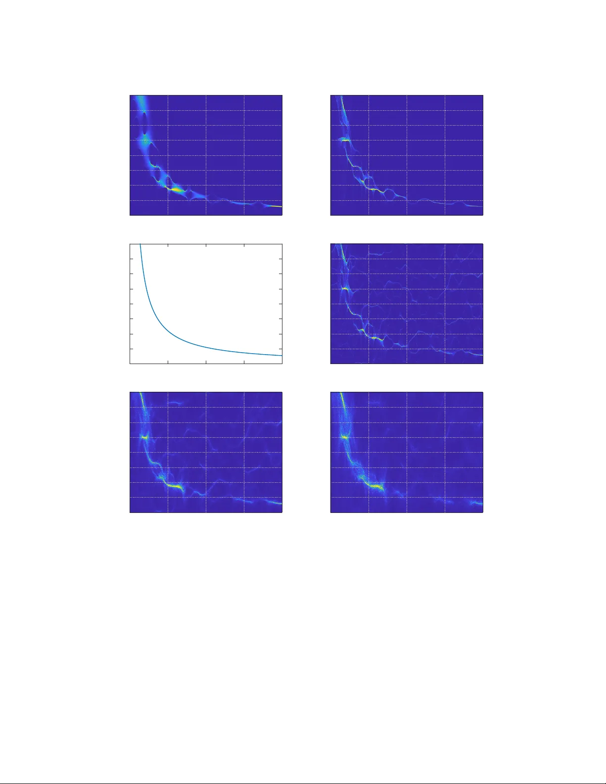
ANAL YZING TRANSIENT-EV OKED OTO A COUSTIC EMISSIONS BY CONCENTRA TION OF FREQUENCY AND TIME HA U-TIENG WU AND YI-WEN LIU Abstract. The linear part of transien t evok ed (TE) otoacoustic emission (O AE) is though t to b e generated via coheren t reﬂection near the characteristic place of con- stituen t wa v e comp onents. Because of the tonotopic organization of the cochlea, high frequency emissions return earlier than low frequencies; how ev er, due to the random nature of coheren t reﬂection, the instan taneous frequency (IF) and amplitude en velope of TEO AEs b oth ﬂuctuate. Multiple reﬂection components and synchronized sp onta- neous emissions can further make it diﬃcult to extract the IF by linear transforms. In this pap er, we prop ose to mo del TEOAEs as a sum of intrinsic mo de-typ e functions and analyze it by a nonlinear-type time-frequency analysis technique called concen- tration of frequency and time (ConceFT). When tested with syn thetic O AE signals with p ossibly multiple oscillatory comp onents, the presen t metho d is able to pro duce clearly visualized traces of individual comp onents on the time-frequency plane. F ur- ther, when the signal is noisy , the prop osed metho d is compared with existing linear and bilinear metho ds in its accuracy for estimating the ﬂuctuating IF. Results suggest that ConceFT outp erforms the b est of these metho ds in terms of optimal transp ort distance, reducing the error by 10 to 21% when the signal to noise ratio is 10 dB or b elo w. 1. INTR ODUCTION T ransient ev ok ed (TE) otoacoustic emissions (TEO AEs) were discov ered 40 years ago Kemp (1978). By insp ecting the wa v eforms, TEOAEs generally exhibit a chirp-like feature in that the high frequency comp onen ts seem to o ccur earlier than low frequency parts. The latency of TEO AE as a function of frequency (hereafter referred to as the latency function ) could p otentially provide v aluable information for hearing diagnostic purp oses b ecause it is, if not directly proportional to, at least highly correlated with the sharpness of co c hlear and psyc hoacoustic tuning (Neely et al. , 1988; Shera et al. , 2002, 2010). Ho w ever, the notion of latency function itself might b e an o v er-simpliﬁcation of the signal of interest for a few reasons. First, the coherent reﬂection theory predicts that the phase in TEOAE sp ectra w ould ﬂuctuate Zweig and Shera (1995); T almadge et al. (2000) b ecause of the random nature in how the trav eling w a ves are scattered in the co c hlea near the characteristic places. The sp ectrum v aries across diﬀeren t ears, and the latency function una voidably has large deviations if directly derived from the phase gradien t (Shera and Bergevin, 2012). Secondly , the reverse tra v eling w a v es in the co c hlea also get reﬂected at the stapes, so the O AE w a v eform measured in the ear canal is a sup erp osition of multiple reﬂections (e.g., see Fig. 8 of T almadge et al. , 1998). T o capture the reﬂections, w e prop ose that TEO AE signals w ould b e represen ted b etter b y a sum of intrinsic mo de typ e (IMT) functions that eac h has time-v arying amplitudes 1 2 HA U-TIENG WU AND YI-WEN LIU T able 1. List of abbreviations AM Amplitude mo dulation BM Basilar membrane ConceFT Concen tration of frequency and time CWD Choi-Williams distribution CWT Con tin uous w a v elet transform IF Instan taneous frequency EMD empirical mo de decomp osition IMT In trinsic mo de type iTFR Ideal time-frequency represen tation MT Multi-tap er RM Reassignment metho d O AE Otoacoustic emission OTD Optimal transp ort distance SNR Signal-to-noise ratio SF O AE Stim ulus frequency O AE SO AE Sp on taneous O AE SPWV Smo othed pseudo Wigner-Ville distribution SSO AE Sync hronized sp on taneous OAE SST Sync hrosqueezing transform STFT Short-time F ourier transform TB T one burst TEO AE T ransient ev ok ed OAE T-F Time-frequency mo dulation and instantaneous frequency . Based on this mo del, we suggest to analyze TEO AE w a veforms by a mo dern time-frequency (T-F) analysis tool called c onc entr ation of fr e quency and time (ConceFT) Daub echies et al. (2016). Mo dern T-F analysis tools could be roughly classiﬁed in to three categories, the linear- t yp e, the bilinear-type and the nonlinear-t yp e. The basic ideas b ehind the linear-t yp e T-F analysis include (i) dividing the signal into segments and ev aluating the sp ectrum for each segmen t (e.g., the Gab or transform or short-time F ourier transform (STFT)) Flandrin (1999), (ii) measuring the similarit y b etw een the signal and a series of di- lations of a given mother w a velet, which leads to the contin uous wa v elet transform (CWT) T ognola et al. (1997); Notaro et al. (2007), or (iii) the S-transform (ST) Mishra and Biswal (2016) that com bines features from STFT and CWT such as frequency mo dulation and dilation. The bilinear-type T-F analysis catc hes signal prop erties from the energy or cross correlation viewp oint, which includes a wide range of metho ds from the traditional Wigner-Ville distribution to the Cohen class Flandrin (1999). The nonlinear-t yp e T-F analysis aims to depict the signal in a more data-driv en wa y , b y either taking more signal information to mo dify the linear-type or bilinear-type T-F analyses, or extracting the information directly from the signal. This category includes the reassignmen t metho d (RM) Auger and Flandrin (1995), the sync hrosqueezing trans- form (SST) Daub ec hies et al. (2011); W u (2011); Ob erlin et al. (2015), the empirical 3 mo de decomp osition (EMD) Huang et al. (1998); Kopsinis and McLaughlin (2009), and sev eral others. W e refer the readers to Flandrin (1999) for a general discussion of a v ailable metho ds and Daub echies et al. (2016) for a recent review of the ﬁeld. Sp eciﬁcally for analyzing TEO AE, Jedrzejczak et al. (2009) built a dictionary of asymmetric Gabor functions to span a linear space and applied matching pursuit al- gorithms to iden tify the b est ﬁt to TEO AEs. The latency function could b e inferred and empirical ﬁts were rep orted. The CWT has b een utilized to see the comp osi- tion or frequency v ariation of the TEOAE T ognola et al. (1997); Notaro et al. (2007), to ﬁlter the OAE signals Jan usausk as et al. (2001); Moleti et al. (2012), to in v esti- gate the relationship of TEO AE latency and stim ulus level Sisto and Moleti (2007), and to infer the hearing functionalit y of neonates (Moleti et al. , 2005; T ognola et al. , 2001). Because of the m ulti-resolution property , CWT pro vides ﬂexibilit y to analyze the frequency latency structure of the OAEs. By ﬁltering on the T-F plane and then applying the inv erse transform, it b ecame also p ossible to separate the ﬁrst-reﬂection comp onen t from its mixture with later reﬂections Shera and Bergevin (2012). Recently , the robustness against noise for v arious time-frequency tec hniques was compared using sim ulated TEO AE data (Bisw al and Mishra, 2017), the tec hniques b eing compared in- cluded STFT, CWT, SST, the S-transform, and EMD; the result suggested that CWT w as the most accurate wa y for estimating the latency function at a signal-to-noise ratio (SNR) of 15 dB. As elegant as the existing T-F analysis tec hniques are, how ev er, there are in trinsic diﬃculties tow ard a deep er insight into the TEOAE. F or the widely applied linear-type T-F analysis, like STFT, CWT and S-transform, the uncertain t y principle Flandrin (1999); Ricaud and T orresani (2014) is inevitable. A direct consequence of the uncer- tain t y principle is a blurring of the sp ectrum, dep ending on the c hosen windo w and its length. Another limitation is its dep endence on the c hosen windo w or mother wa v elet and lack of the adaptivity to the signal. F or example, while w e can take the frequency latency property of TEOAE signal in to accoun t and design a mother w a v elet to well trac k that part T ognola et al. (1997); Sisto et al. (2015), when there are other com- p onen ts in the recording, suc h as the sync hronized sp ontaneous O AE (SSO AE) (e.g., discussed b y Keefe, 2012), we migh t need another mother w a velet to catc h them. In short, ho w to c ho ose a univ ersal mother w a v elet to accomo date signals of diﬀeren t fea- tures is in general challenging for the linear metho d, and this could also c hallenge the in terpretation of the outcomes. While the bilinear-type T-F analysis has a p oten tial to alleviate these limitations, it suﬀers from diﬀeren t limitations. F or example, while the adaptivity issue is resolved b y taking the signal itself as the windo w in the traditional Wigner-Ville distribution, it is limited by the in terference terms when the signal is comp osed of m ultiple oscilla- tory comp onen ts or time-v arying frequency . F or other commonly applied Cohen class algorithms, like Choi-Williams distribution (CWD) or Smo othed pseudo Wigner-Ville distribution (SPWV), the same interference issue p ersists. When choosing windo ws for smo othing is needed, the same interpretation issue for the linear metho d still stands. F urthermore, when time information is touc hed during smo othing, it is diﬃcult to preserv e causality . 4 HA U-TIENG WU AND YI-WEN LIU Among diﬀerent nonlinear-type T-F analyses, the widely applied EMD lacks of the- oretical foundation and migh t lead to erroneous in terpretation and conclusion for real data. RM and SST, on the other hand, hav e been developed rigorously with theoretical supp ort to handle the traditional T-F analysis limitations. In particular, b y taking the phase information of the signal in to accoun t, the spectrum is sharp ened b ey ond the blurriness limit caused by the uncertain principle, and the resulting T-F representation is less dep enden t on the chosen windo ws Daub ec hies et al. (2011); W u (2011); Ob erlin et al. (2015). Depending on ho w the phase information is used, SST can b e classiﬁed in to ﬁrst W u (2011) or second Ob erlin et al. (2015) order. The ﬁrst order SST is limited to signals with slowly v arying frequency and the second order SST is designed to handle fast v arying frequency situation. While it is a nonlinear method, it is sho wn in Chen et al. (2014) that the ﬁrst order SST is robust to reasonable amount of diﬀeren t t yp es of noise, including the non-stationary and heteroscedastic kinds. How ev er, when the signal to noise ratio (SNR) is low (e.g., below 2 dB), the nonlinear-t yp e T-F analyses in general do es not p erform w ell. T o sum up, while there hav e b een sev eral T-F anal- ysis techniques, it is still a long lasting challenge to study the TEOAE signal, due to (i) its intrinsic oscillatory structure predicted b y theory , (ii) the existence of m ultiple reﬂection comp onen ts or ev en sync hronized spontaneous emissions Keefe (2012), and (iii) the lo w SNR encoun tered in practice. T o handle these challenges, in this pap er, we explore the p ossibilit y of analyzing TEO AEs by ConceFT Daubechies et al. (2016), which is a nonlinear-t yp e T-F tech- nique that extends the RM and SST b y com bining the multi-tap ering (MT) tec hnique. It has b een established that, if the signal of interest can b e mo deled as a sum of IMT functions satisfying a wel l-sep ar ate d condition and certain slow-varying assumptions, then ConceFT helps pro duce sharp ened traces on the T-F plane that represent the signal and are robust to noise Daubechies et al. (2016). The basic idea b ehind Con- ceFT is tw ofold. First, a nonlinear-t ype T-F analysis is chosen, like SST or RM, and the sharp ened time-frequency representation pro vides higher ﬁdelit y to the sp ectral con ten t of the signal. Second, the eﬀects of noise in O AE measuremen t are reduced b y generalizing the traditional MT technique Perciv al and W alden (1993); Daub echies et al. (2016), which b eneﬁts directly from the nonlinearity of the sharp ening pro cedure. T o understand which kind of information ConceFT could accurately extract, we adopt tw o diﬀerent mo dels to sim ulate TEO AE in a con trolled manner, so that we can ev aluate the p erformance of ConceFT analysis thoroughly and understand what are the conditions for it to w ork w ell on TEO AEs. In one mo del, the TEO AE spectrum is expressed in terms of a direct in tegral that takes the presence of irregularit y into accoun t Shera and Bergevin (2012); Zweig and Shera (1995). In the other model Liu and Neely (2010), irregularities are presen t in ph ysical v ariables suc h as the basilar- mem brane mass, damping co eﬃcients, and stiﬀness, and TEOAEs are “measured” b y time-domain simulation. Lastly , w e quantify the p erformance and compare ConceFT with other T-F analysis tools on a fully simulated signal that w e know the ground truth. The organization of the rest of this paper is as follows. Sec. 2 introduces SST and ConceFT in details. Sec. 3 sho ws the results of applying SST and ConceFT to analyze 5 syn thetic TEOAE data. Based on the results of simulation, Sec. 4 discusses the eﬀec- tiv eness and limitation of the prop osed signal analysis approach. Conclusions are given in Sec. 5. 2. Concentra tion of frequency and time Based on the literature review, w e understand that a TEO AE signal ma y contain m ultiple reﬂection comp onen ts or ev en SSO AEs. W e suggest that it w ould b e ap- propriate to mo del eac h comp onen t with time-v arying amplitude and frequency . T o capture these, we resort to the in trinsic mo de t yp e (IMT) function Daubechies et al. (2011) deﬁned as follows, f ( t ) = A ( t ) e iφ ( t ) , where A ( t ) and φ ( t ) satisfy the following three conditions. The ﬁrst condition is the r e gularity condition; that is, A and φ are smo oth enough. The second one is the b ounde dness condition; that is, b oth A ( t ) and φ 0 ( t ) are strictly p ositive and bounded from abov e. The third one is the slow ly varying condition; that is, w e could ﬁnd constan ts ε 1 , ε 2 > 0 so that | A 0 ( t ) | ≤ ε 1 | φ 0 ( t ) | and | φ 00 ( t ) | ≤ ε 2 | φ 0 ( t ) | for all t . 1 W e refer to A ( t ) as the amplitude mo dulation (AM) or amplitude env elope of f ( t ), φ ( t ) the phase function of f ( t ), and φ 0 ( t ) the (angular) instantane ous fr e quency (IF) of f ( t ). The regularit y , b oundedness and slowly-v arying conditions say that locally an IMT function b eha ves lik e a sin usoidal function. The slowly v arying IF condition can b e sligh tly relaxed Oberlin et al. (2015); Kow alski et al. (2018) to accommo date fast v arying IF lik e c hirps, but to simplify the discussion, w e fo cus on the slo wly v arying conditions. Note that this mo del satisﬁes the identiﬁabilit y condition Chen et al. (2014); that is, if w e could ﬁnd a ( t ) and ψ ( t ) that satisfy f ( t ) = A ( t ) e iφ ( t ) = a ( t ) e iψ ( t ) , then a ( t ) = A ( t ), and ψ ( t ) = φ ( t ) up to a global diﬀerence of an in teger m ultiple of 2 π for all time t . This can b e easily seen by taking the absolute v alue and hence un wrapping the phase. Note that although the IMT function is written in the complex form, it is in general not analytic, since the F ourier transform of an IMT function might not b e supp orted on the p ositiv e axis due to the time-v arying amplitude and frequency . W e th us mo del the TEOAE signal as a sum of several IMF functions, with diﬀeren t AM and IF functions. F or instance, when only t w o comp onen ts are considered, the adaptiv e harmonic mo del has the follo wing expression, (1) f ( t ) = A 1 ( t ) e iφ 1 ( t ) + A 2 ( t ) e iφ 2 ( t ) , where A 1 ( t ) e iφ 1 ( t ) ma y mo del the dominant ﬁrst-reﬂection comp onent of TEOAE and A 2 ( t ) e iφ 2 ( t ) mo dels the second reﬂection. In this setu p, we need the fr e quency sep ar ation condition; that is, φ 0 1 ( t ) − φ 0 2 ( t ) ≥ d > 0 W u (2011), or φ 0 1 ( t ) − φ 0 2 ( t ) ≥ d ( φ 0 1 ( t ) + φ 0 2 ( t )) Daub ec hies et al. (2011). Diﬀerent linear T-F analysis tool needs diﬀeren t frequency separation prop erties, dep ending on the frequency mo dulation or dilation nature of the T-F analysis; φ 0 1 ( t ) − φ 0 2 ( t ) ≥ d > 0 is needed if STFT is considered, and φ 0 1 ( t ) − φ 0 2 ( t ) ≥ d ( φ 0 1 ( t ) + φ 0 2 ( t )) is needed if CWT is considered. The frequency separation condition is 1 Note that this deﬁnition is sligh tly diﬀerent from that giv en in Daub echies et al. (2011), where ε 1 = ε 2 , since for a practical signal, lik e TEOAE, the ph ysical units of A ( t ) and φ 0 ( t ) migh t be diﬀeren t. This unit issue could b e taken care by ε 1 and ε 2 . 6 HA U-TIENG WU AND YI-WEN LIU needed for the iden tiﬁabilit y condition to b e satisﬁed Chen et al. (2014); Ob erlin et al. (2015); Kow alski et al. (2018). If a TEOAE signal can b e mo deled as a sum of IMT functions, several mo dern nonlinear-t yp e T-F analysis to ols can b e applied with theoretical guaran tees. P artic- ularly , w e can apply the RM or SST to analyze the TEOAE signal and exp ect to get the IF and AM information back Daub echies et al. (2011). 2 F urther, when the SNR is lo w, w e could consider the MT technique Perciv al and W alden (1993); Xiao and Flandrin (2007) to stabilize the noise impact. A com bination of nonlinear-type T-F analysis to ols, like SST, and MT tec hniques is called c onc entr ation of fr e quency and time (ConceFT). The SST and the MT tec hniques are describ ed next, resp ectively . 2.1. Sync hrosqueezing transform. The basic idea b ehind SST is taking the phase information hidden inside the c hosen T-F representation, lik e STFT W u (2011), CWT Daub ec hies et al. (2011) or S-transform Huang et al. (2016), and shuﬄing the T-F represen tation co eﬃcien ts to alleviate the blurring eﬀect caused by the uncertain t y principle. Sp eciﬁcally , SST is comp osed of three steps. Belo w, we discuss SST based on STFT, and the discussion for CWT or S-transform can b e found in Daub ec hies et al. (2011); Huang et al. (2016). First, for a given prop erly deﬁned function f , the STFT asso ciated with a window function h ( t ) is deﬁned by (2) V ( h ) f ( t, ν ) := Z f ( τ ) h ( τ − t ) e − i 2 π ν ( τ − t ) d τ , where t ∈ R is the time, ν = ω / 2 π ∈ R + is the frequency , h is the window func- tion c hosen by the user — a common choice is the Gaussian function, i.e. h ( t ) = (2 π σ ) − 1 / 2 e − t 2 / 2 σ 2 , where σ > 0. T o sharp en the sp ectrogram | V ( h ) f ( t, ν ) | 2 , note that the phase information of V ( h ) f ( t, ν ) is not used. A keen observ ation made in Ko dera et al. (1978); Auger and Flandrin (1995); Flandrin (1999) is that the geometric and phase information in the T-F represen tation allows us to sharp en it. T o motiv ate this k een observ ation, consider a simple function f ( t ) = Ae i 2 π f 0 t , where A , f 0 > 0. By a direct calculation, V ( h ) f ( t, ν ) = A ˆ h ( ν − f 0 ) e i 2 π f 0 t , where ˆ h := F [ h ( t )]. Note that the frequency f 0 sho ws up in the phase of V ( h ) f ( t, ν ). A na ¨ ıv e idea to obtain the frequency information thus consists of t wo steps: ﬁrst, the partial deriv ativ e of V ( h ) f ( t, ν ) asso ciated with t is calculated, which giv es ∂ t V ( h ) f ( t, ν ) = i 2 π f 0 A ˆ h ( ν − f 0 ) e i 2 π f 0 t , and then the frequency f 0 can b e retriev ed b y a direct division; that is, (3) f 0 = ∂ t V ( h ) f ( t, ν ) i 2 π V ( h ) f ( t, ν ) . 2 In reality , TEOAE signals are real-v alued, and Hilb ert transform has b een applied to construct an IMT from its real part Keefe (2012). In con trast, the RM or SST metho ds do not require Hilb ert transform to tak e place because they can handle concurrents IMFs, including the sp ecial case of cos φ ( t ) = 1 2 ( e iφ ( t ) + e − iφ ( t ) ). 7 T o a v oid calculating the n umerical deriv ativ e ∂ t V ( h ) f ( t, ν ), note that (4) ∂ t V ( h ) f ( t, ν ) = − V ( D h ) f ( t, ν ) + i 2 π ν V ( h ) f ( t, ν ) , where D h denotes the deriv ativ e of h with resp ect to time. W e th us ha v e V ( D h ) f ( t, ν ) = i 2 π ( ν − f 0 ) V ( h ) f ( t, ν ) = i 2 π A ( ν − f 0 ) ˆ h ( ν − f 0 ) e i 2 π f 0 t . This observ ation motiv ates the deﬁnition of the following r e assignment rule (W u, 2011, Deﬁnition 2.3.12), (5) ω ( h ) f ( t, ν ) := ν − Im V ( D h ) f ( t, ν ) 2 π V ( h ) f ( t, ν ) , where Im means taking the imaginary part. Equation (5) is well-deﬁned on ev ery points ( t, ν ) where V ( h ) f ( t, ν ) 6 = 0. T o sharp en the T-F representation of V ( h ) f ( t, ν ), an in tuitiv e approac h is, for each time t , mo ving all coeﬃcients to the en try asso ciated with the frequency w e hav e in terest. This intuition is carried out in SST b y the follo wing integration form ula (W u, 2011, Deﬁnition 2.3.13): (6) s ( h ) f ( t, ν ) := Z N t V ( h ) f ( t, ν 0 ) δ | ν − ω ( h ) f ( t,ν 0 ) | d ν 0 , where N t := { ν 0 : | V ( h ) f ( t, ν 0 ) | > 0 } . Equation (6) can b e understo o d as a combination of tw o steps: • First, ﬁnd all entries ( t, ν 0 ) so that the frequency information provided b y ω ( h ) f ( t, ν 0 ) is ν , which is embo died in δ | ν − ω ( h ) f ( t,ν 0 ) | . 3 • Secondly , gather all non-zero STFT co eﬃcients to the entry ( t, ν ) by the in te- gration. In the simple example f ( t ) = Ae i 2 π f 0 t , the non-zero STFT co eﬃcients are all mo v ed to f 0 in s ( h ) f ( t, ν ), resulting a sharp T-F representation. As is sho wn in (W u, 2011, Theorem 2.3.14), SST can b e applied to study IMT functions. F or f ( t ) = A ( t ) e iφ ( t ) , the sharp ened sp ectrogram b y SST (that is, | s ( h ) f ( t, ν ) | 2 ) is concen trated on φ 0 ( t ) / 2 π with the AM function A ( t ) enco ded inside. As a result, this tec hnique alleviates the blurring eﬀect caused b y the uncertaint y principle. Ho w ever, when the IF of an IMT function c hanges rapidly , the outcome of the ab ov e- men tioned SST b ecomes less ideal b ecause the reassignmen t rule is again “blurred”. Certain improv emen t has b een found by Ob erlin et al. (2015) via further manipulation of the phase function to accommo date the fast-v arying IF; the follo wing reassignment rule was in tro duced, Ω ( h ) f ( t, ν ) = ( ω ( h ) f ( t, ν ) + Q ( h ) f ( t, ν )( t − T ( h ) f ( t, ν )) when ∂ ν T ( h ) f ( t, ν ) 6 = 0 ω ( h ) f ( t, ν ) otherwise , (7) 3 T o make it mathematically rigorous, the delta measure should b e replaced by a smo oth appro xi- mation. W e skip the technical detail here for the simplicity . 8 HA U-TIENG WU AND YI-WEN LIU where Q ( h ) f ( t, ν ) := V ( DD h )( t,ν ) f ( t, ν ) V ( h ) f ( t, ν ) − ( V ( D h ) f ( t, ν )) 2 2 π i [( V ( h ) f ( t, ν )) 2 + V ( T h ) f ( t, ν ) V ( D h ) f ( t, ν ) − V ( T D h ) f ( t, ν ) V ( h ) f ( t, ν )] T ( h ) f ( t, ν ) := t + Re V ( T h ) f ( t, ν ) V ( h ) f ( t, ν ) , (8) Q f and T f are deﬁned when their denominators are not zero, Re means taking the real part, and ( T h )( t ) := th ( t ). Ω ( h ) f is called the se c ond-or der fr e quency r e assignment rule Ob erlin et al. (2015). With this terminology , we ma y call ω ( h ) f the ﬁrst-or der fr e quency r e assignment rule W u (2011). With the second-order frequency reassignment rule, the second order STFT-based SST is deﬁned as: (9) S ( h ) f ( t, ν ) := Z N t V ( h ) f ( t, ν 0 ) δ | ν − Ω ( h ) f ( t,ν 0 ) | d ν 0 . Again, we ma y call s ( h ) f ( t, ν ) the ﬁrst-order STFT-based SST. Note that, for b oth ﬁrst and second order STFT-based SST, we nonlinearly reassign the STFT co eﬃcient only on the frequency axis, so the causalit y of the signal is preserved and hence the reconstruction is p ossible, although we do not pursue these prop erties in this work. Y et another prop erty of ﬁrst-order SST is its robustness to noise of diﬀeren t kinds Thakur et al. (2013); Chen et al. (2014), while it is nonlinear in nature. The ab ov e prop erties enable us to extract dynamical information of a noisy oscillatory signal, particularly the IF and AM. In this work, due to the c hirp-lik e behavior of the TEO AE signal, we consider the second-order STFT-based SST for the analysis. With no danger of confusion, w e call it SST for simplicity b elo w, unless we sp ecify that it is the ﬁrst order SST. Note that CWT-based SST can also b e considered Daub echies et al. (2011) for the analysis, but to simplify the discussion, w e fo cus only on the STFT-based SST. 2.2. Generalized m ulti-tap er. While the ﬁrst order SST is theoretically shown to b e robust to a mild lev el of noise Thakur et al. (2013); Chen et al. (2014), when the noise is large, its p erformance migh t b e jeopardized. While theoretical analysis for other nonlinear-t yp e T-F analysis to ols are not av ailable, empirically they are robust only when noise lev el is mild. In practice, the TEO AE obtained within a limited amount of time could b e noisy with a rather small SNR. Th us, a tec hnique to reduce the eﬀect of noise w ould b e desired. In this work, we consider the recen tly prop osed generalized MT technique Daub ec hies et al. (2016) to ac hiev e this goal. The spirit of the traditional MT technique roots in the law of large num bers. Ideally , from a recorded noisy signal, if we can generate sev eral copies of information comp osed of the clean component and independent noise, b y taking a verage the clean signal will b e enhanced. This intuitiv e idea is carried out in the follo wing w a y . With the c hosen orthonormal windo ws, the obtained sp ectral information asso ciated with the clean signal is almost inv ariant among windo ws, while that asso ciated with the noise is indep enden t. F or example, tak e a noisy signal giv en as Y = f + ξ , where f is the 9 signal w e hav e interest and ξ is the added noise, and take J orthonormal windo ws h j , j = 1 , . . . , J . By the linearity of STFT, w e hav e V ( h j ) Y ( t, η ) = V ( h j ) f ( t, η ) + V ( h j ) ξ ( t, η ), for i = 1 , . . . , J . When ξ is Gaussian and white, we see that V ( h j ) ξ ( t, η ) and V ( h k ) ξ ( t, η ) are indep endent when j 6 = k . While the sp ectral information asso ciated with V ( h j ) f ( t, η ) dep ends on h j , by the linearit y of STFT again, 1 J P J j =1 V ( h j ) f ( t, η ) = V ( 1 J P J j =1 h j ) f ( t, η ). Therefore, b y taking an a v erage, only the spectral information associated with the clean signal is reserv ed. The T-F representation of SST can be impro v ed b y the MT tec hnique b y considering (10) M Y := 1 J J X j =1 S ( h j ) Y . In Lin et al. (2014), the MT tec hnique combined with SST is applied to study the anesthesia depth. The combination of the MT tec hnique and RM is considered in Xiao and Flandrin (2007). Ideally , if there are inﬁnitely many orthonormal functions “w ell supp orted” in time and frequency domains, the MT technique would lead us to a low bias and lo w v ariance estimator of the clean signal information. Ho wev er, it has b een w ell studied in Daub ec hies (1988) that the n um ber of orthonormal functions that are w ell concen trated in the T-F plane is limited. This fact is understo o d as the “Nyquist rate” for the T-F analysis. 4 T o conquer the limitation of Nyquist rate and further stabilize the algorithm, the nonlinear nature of SST is considered. Ho w ConceFT generalizes the ab o ve-men tioned traditional MT technique could b e manifested by directly showing the algorithm. Con- sider a linear combination of given J orthonormal windows h j , j = 1 , . . . , J , h = r ∗ H , where H = [ h 1 , . . . , h J ] T , r = [ r 1 , r 2 , ..., r J ] ∈ C J and | r | = 1, we could obtain a T-F represen tation, denoted as S ( h ) Y , b y applying the SST. Note that when r = e j is the unit vector with the j -th entry equal to 1, r ∗ H = h j . The T-F representation based on ConceFT is deﬁned as (11) C Y := 1 N N X n =1 S ( h ( n ) ) Y where r ( n ) is uniformly sampled from the unit sphere in C J and h ( n ) := r ∗ ( n ) H . In tuitiv ely , due to the nonlinear nature of SST, the level of dep endence is reduced b et ween noise comp onen ts coming from non-orthogonal windows. Thus, by taking a v erage, the noise could b e further canceled. T o appreciate the imp ortance of the nonlinearit y , take the follo wing examples in to account. If w e consider the linear-type T-F analysis, like the STFT, and follo w the ab ov e-men tioned argument regarding 4 The “Nyquist rate” here is diﬀeren t from the common Nyquist rate encountered in the sampling theory . Here, it is called the Nyquist rate to describ e limited p ossible windows under the constrain ts suc h as orthonormalit y and well concentration. See Daub echies (1988) for a full dev elopmen t and (Daub ec hies et al. , 2016, ESM-4) for a summary . 10 HA U-TIENG WU AND YI-WEN LIU generalized MT, w e hav e (12) lim N →∞ 1 N N X n =1 V ( h ( n ) ) Y = lim N →∞ 1 N N X n =1 J X j =1 e > j r ( n ) V ( h j ) Y = J X j =1  lim N →∞ 1 N N X n =1 e > j r ( n )  V ( h j ) Y = 0 due to the linearity of STFT. Here we use the fact that lim N →∞ 1 N N X n =1 e > j r ( n ) = e > j Z x ∈ C J ; k x k =1 xdx = 0 . F urther, if we apply the generalized MT to the sp ectrogram, we ha ve lim N →∞ 1 N N X n =1 | V ( h ( n ) ) Y | 2 = lim N →∞ 1 N N X n =1 | J X j =1 e > j r ( n ) V ( h j ) Y | 2 = J X j =1  lim N →∞ 1 N N X n =1 | e > j r ( n ) | 2  | V ( h j ) Y | 2 + J X j 6 = k  lim N →∞ 1 N N X n =1 ( e > j r ( n ) ) ∗ e > k r ( n )  V ( h j ) Y ∗ V ( h k ) Y = c 1 J J X j =1 | V ( h j ) Y | 2 , for some constan t c > 0, where the last equalit y comes from the fact that lim N →∞ 1 N N X n =1 | e > j r ( n ) | 2 = Z x ∈ C J ; k x k =1 | x j | 2 dx = c and lim N →∞ 1 N P N n =1 ( e > j r ( n ) ) ∗ e > k r ( n ) = R x ∈ C J ; k x k =1 x ∗ j x k dx = 0 due to the symmetry since j 6 = k . Thus, the generalized MT technique leads to the traditional MT on the sp ectrogram. The same discussion holds for CWT and scalogram. Ho w ever, the situation is diﬀerent when w e apply the generalized MT tec hnique to an y nonlinear-type T-F analysis. F or example, due to the nonlinearity of the SST, lim N →∞ C Y is not proportional to M Y , since S ( h ( n ) ) Y 6 = P J j =1 e > j r ( n ) S ( h j ) Y . In brief, due to the Nyquist rate limitation, w e choose a reasonably small J , and coun t on a large N to reject the noise. Although a complete theoretical quantiﬁcation is still under study , a partial theoretical result and n umerical evidence in Daub ec hies et al. (2016) sho w that the level of dep endence betw een noise comp onen ts caused by tw o non- orthonormal windo ws is reduced after SST. As a result, lim N →∞ C Y is m uc h closer to S f than M Y is, when measured by the optimal transp ortation distance Daub echies et al. (2016). W e also men tion that the generalized MT technique could b e applied to other nonlinear-type T-F analysis, lik e RM. In practice, w e choose h 1 , . . . , h J to b e the ﬁrst J orthonormalized Hermite functions b ecause they are the most concen trated windo ws in the T-F domain Daub echies (1988); Daub ec hies et al. (2016). In particular, h 1 is the Gaussian function. In practice, J could b e chosen as small as 2, while N could b e c hosen as large as the user wishes, but a n um b er of N = 30 to 100 is in general go o d enough (e.g. Daub echies et al. , 2016). 11 3. Comp arison of v arious w a ys to anal yze TEO AE da t a In this section, w e rep ort results of analyzing sim ulated TEOAE data by sync hrosqueez- ing and ConceFT. The p erformance will b e compared against what can b e ac hiev ed by linear analysis metho ds, including STFT and CWT, and bilinear metho ds lik e CWD and SPWV. 3.1. Direct simulation of coheren t reﬂection. This section follows Zw eig and Shera’s c oher ent r eﬂe ction approac h to simulate a TEOAE signal (1995). Essentially , the TEO AE is regarded as the summation of reﬂected w av es caused by mec hani- cal irregularities throughout the entire length of the co chlea, whic h is treated as a one-dimensional w av eguide. Via W entzel-Kramers-Brillouin (WKB) appro ximation Sc hro eder (1973), Zweig and Shera show ed that the amoun t of reﬂection can b e com- puted b y introducing the irregularities to the wa v e propagation equation as a p ertur- bation term. This framework successfully explained the perio dic ﬁne structure in the sp ectrum of diﬀerent t yp es of OAEs and the hearing threshold T almadge et al. (1998). Here, w e b orro w a phenomenological equation that stems from the 1995 work for synthe- sizing a TEO AE signal without discussing the details of micromechanics of the cochlea. The reﬂection of trav eling w a v es in the cochlea due to unkno wn irregularities  ( x ) is written as follows (T almadge et al. , 2000; Shera and Bergevin, 2012; Bisw al and Mishra, 2017), (13) R ( ω ) = Z  ( x 0 ) e − ( x 0 − x p ) 2 2(∆ x ) 2 e − i 4 π x 0 − x p Λ dx 0 , where ω > 0, ∆ x represents a spatial spread of a tra v eling w a v e near its characteristic place, and Λ denotes the lo cal w a v elength. Here, R ( ω ) represents a reﬂectance sp ectrum “seen” from the stap es ( x = 0) into the co c hlea. In the equation, x p denotes the char acteristic plac e of (angular) frequency ω and is assumed to decrease against ω in a log-linear wa y as follows (Green woo d, 1990), (14) x p ( ω ) = l log ω 0 ω , where l is treated as a constant here, and ω 0 is the characteristic frequency at x = 0. In Eq. (13), the factor exp  − ( x 0 − x p ) 2 2(∆ x ) 2  describ es the relativ e gain a small w av e comp onent receiv es by going from x = 0 to x = x 0 and reﬂected to trav el bac k to x = 0, and the factor exp {− i 4 π ( x 0 − x p ) / Λ } corresp onds to the phase-shift thereof. In Eq. (13), R ( ω ) is zero if  ( x ) = 0, meaning that TEOAE w ould not exist if the co c hlea were to be p erfectly smo oth. By ﬁtting exp erimental data, it has been found that ∆ x and Λ should both v ary slo wly against ω (Shera and Bergevin, 2012). Here, ho w ev er, w e set b oth of them as constan ts; in other words, we made a crude simpliﬁcation of co chlear mechanics so the mo del has a global scaling symmetry . Also, w e regard the in verse F ourier transform 5 r ( t ) = F − 1 [ R ( ω )]( t ) as a impulse resp onse, which can be con v olv ed with any transien t acoustic stim ulus to calculate 5 The in verse F ourier transform was calculated via a 4096-point inv erse fast F ourier transform with a sampling rate of 32 kHz. 12 HA U-TIENG WU AND YI-WEN LIU the ﬁrst-reﬂection O AE evok ed b y the stim ulus. 6 Th us, we ignore multiple in ternal reﬂection in the co c hlea due to imp edance mismatch at the stap es. The frequency resp onse of rev erse middle-ear transmission, the ear-canal acoustics, and the acoustic prop erties of the prob e termination are also ignored, to o. The mo del in Sec. 3.2 w ill consider b oth the multiple reﬂections in the co c hlea and the middle-ear transmission, and restrict scaling symmetry to b e v alid only lo cally . Here in Sec. 3.1, the reason for making these crude simpliﬁcations are tw o-fold. First, we shall see that the ﬁrst-reﬂection comp onent already demonstrates ﬂuctuating AM and IF and presen ts a challenge for data analysis. Therefore, w e shall use the synthesized r ( t ) to help determining ConceFT parameters empirically . Secondly , the global-symmetry assumption happ ens to allo w certain appro ximations that lead a simpler expression for r ( t ). It turns out that the level of temporal ﬂuctuation in the AM and IF of r ( t ) closely dep ends on the ratio ∆ x/ Λ. Details of mathematical deriv ation are giv en in App endix B, C, and D, and related discussion will b e giv en in Sec. 4. 3.1.1. Cho osing the SST and MT p ar ameters. An example of R ( ω ) was syn thesized via Eq. (13) with the follo wing parameters: l = 0 . 72 cm, Λ = l / 5 . 5 (Shera and Bergevin, 2012), and ∆ x = Λ / 2. The irregularit y function  ( x ) was generated by a zero-mean Gaussian random pro cess with a constan t v ariance E[  ( x )] 2 = σ 2  and no spatial corre- lation; i.e., E {  ( x )  ( x 0 ) } = 0 if x 6 = x 0 . The integral with resp ect to x 0 in Eq. (13) w as appro ximated b y discretizing along the x 0 direction from x 0 = 0 to 35 mm with a step size of 5 µ m. The resulting R ( ω ) was calculated in the frequency domain from 0.2 to 16 kHz and the in v erse fast F ourier transform w as applied to obtain the TEOAE signal r ( t ) sampled at f s = 32 kHz. Then, Re { r ( t ) } was sub ject to further analyses. T o test the robustness of the signal-pro cessing metho ds, Gaussian white noise ξ ( t ) ∼ N (0 , σ 2 ξ ) w as added to Re { r ( t ) } . Figure 1 sho ws Re { r ( t ) } b efore and after con taminated by the noise. This signal is further analyzed as b elow. An STFT sp ectrogram V ( h ) f of signal f ( t ) = Re { r ( t ) } w as calculated using the Gauss- ian windo w function h ( t ) with σ = (5ms) / 12. Then, b oth the 1st-order and the 2nd- order SST w ere tried for comparison purp oses, and the resulting T-F representations S ( h ) f ( t, ν ) are shown in Fig. 2A and B. The exp e cte d instantaneous frequency (EIF) function is plotted in Fig. 2C as a reference; The EIF function, denoted as ¯ ν ( t ), is es- sen tially deﬁned as the inv erse function of the exp ected group delay 7 giv en by Eq. (23); to b e exact, we deﬁne that E { τ g  2 π ¯ ν ( t )  } = t , and therefore, (15) ¯ ν ( t ) = 1 2 π 4 π t  l Λ  = 2 t  l Λ  = 11 . 0 /t, where the unit of t is sec and the unit of ¯ ν is Hz. Note that in Fig. 2A and B, b oth the 1st and the 2nd order SST pro duce traces that generally follo w Eq. (15) but with blurring and deviation. The bac kground is clean in b oth cases b ecause the noise has not b een added yet. Also note that, compared to the 1st-order SST, the trace in the 2nd-order SST app ears to b e more concentrated when 6 Of course, this w ould no longer b e v alid if nonlinearity in co chlear mec hanics is considered. 7 In h uman data, the in verse relation was ﬁnd to hold for a limited p erio d of time, from about t = 3 to 8 ms Keefe (2012). 13 0 5 10 15 20 25 30 Time (ms) -1 -0.5 0 0.5 1 arbitrary unit 10 -3 (A) 0 5 10 15 20 25 30 Time (ms) -5 0 5 arbitrary unit 10 -4 (B) Figure 1. Signals generated b y Eq. (13) for further analysis. (A) the real part of the clean TEOAE signal r ( t ). (B) Contaminated by Gaussian noise with σ ξ = 4 . 7 × 10 − 5 . the IF changes fast, as was predicted by the established theorem Daub ec hies et al. (2011); Ob erlin et al. (2015). F or this reason, the 2nd-order SST is chosen as the to ol for analyzing the signals further. Fig. 2D sho ws the 2nd-order SST of the con taminated signal f ( t ) = Re { r ( t ) } + ξ ( t ) (See Fig. 1B). By insp ection and comparing with Fig. 2B, we can ﬁnd sev eral spurious traces in the upp er-righthand side of the “main trace” due to the additive noise (the main trace is v aguely deﬁned as the set of all visible traces lo cated close to ν = ¯ ν ( t ) on the T-F plane). Fig. 2E and F show the result of further pro cessing by ConceFT using the ﬁrst J = 2 and 3 Hermite basis functions, resp ectiv ely . The n um b er of av erages in Eq. (11) is N = 90. Note that, b efore time t = 10 ms, the the main trace app ears to b e preserv ed in b oth Fig. 2E and F. A t time t > 10 ms, how ev er, the main trace app ears to b e harder to identify , especially b etw een t = 10 and 13 ms. In fact, the global scaling symmetry assumption in this mo del predicts that the TEOAE amplitude w ould deca y fast; and w e attempt to pro vide a mathematical explanation for the reasons in App endix D. Consequently , it becomes harder to see the tracing at later time as the signal level ev en tually drops b eneath the noise ﬂo or. Also note that the spurious traces due to the presence of noise app ear to b e suppressed b etter when using J = 3 Hermite functions (Fig. 2F) than J = 2 (Fig. 2E), and this impro v ed p erformance p ossibly comes with the price of low ering the visibility of the main trace when the SNR is b elo w a certain limit, e.g., around t = 12 and also t = 17 ms, resp ectively . 14 HA U-TIENG WU AND YI-WEN LIU (A) 0 5 10 15 20 Time (ms) 0 1 2 3 4 5 6 7 8 Frequency (kHz) (B) 0 5 10 15 20 Time (ms) 0 1 2 3 4 5 6 7 8 Frequency (kHz) 0 5 10 15 20 Time (ms) 0 1 2 3 4 5 6 7 8 Frequency (kHz) (C) (D) 0 5 10 15 20 Time (ms) 0 1 2 3 4 5 6 7 8 Frequency (kHz) (E) 0 5 10 15 20 Time (ms) 0 1 2 3 4 5 6 7 8 Frequency (kHz) (F) 0 5 10 15 20 Time (ms) 0 1 2 3 4 5 6 7 8 Frequency (kHz) Figure 2. (Color online) Results of representing sim ulated TEOAE sig- nals b y SST and ConceFT. (A) 1st-order SST, clean signal. (B) 2nd- order SST, clean signal. (C) The exp e cte d instantaneous frequency (see Eq. 15 for the deﬁnition) as a function of time. (D) 2nd-order SST, noise con taminated. (E) ConceFT with J = 2 and N = 90. (F) ConceFT with J = 3 and N = 90. 3.1.2. R esults with a mor e r e alistic value of ∆ x/ Λ . Based on Eq. (13), w e will show in App endix B and C that the O AE signal, b ( t ), ev oked b y a narro wband stim ulus g ( t ) 15 0 5 10 15 20 25 30 Time (ms) -6 -4 -2 0 2 4 arbitrary unit 10 -4 (A) (B) 0 5 10 15 20 Time (ms) 0 1 2 3 4 5 6 7 8 Frequency (kHz) Figure 3. (Color online). Results with a more realistic v alue of ∆ x . (A) r ( t ) with ∆ x = l / ( √ 2 π 10) ≈ 0 . 22Λ, as in Shera and Bergevin (2012) and Bisw al and Mishra (2017). (B) the corresp onding 2nd-order SST, obtained with a Gaussian windo w σ = 0 . 167 ms. that is cen tered around frequency ω b could b e appro ximated as follows, (16) b ( t ) ≈ C 00 R ( ω b ) · g  t − 4 π Λ l ω b  , where C 00 = e i 4 π Λ l represen ts a constan t phase shift that do es not dep end on ω b , and R ( ω b ) dep ends on the irregularity function  ( x ) is given by Eq. (13). How ev er, the go o dness of approximation of Eq. (16) relies on ∆ x/ Λ b eing suﬃcien tly large, and it can b e exp ected that the b ehaviors of TEOAE b ecome more diﬃcult to capture when ∆ x/ Λ is low. The go o dness of approximation b y Eq. (16) and implications will b e further discussed in Sec. 4. Fig. 3 shows the result of simulating r ( t ) with a more reasonable v alue of ∆ x/ Λ (Shera and Bergevin, 2012; Biswal and Mishra, 2017) inferred from exp eriments (Rho de, 1978). T o simplify the discussion, no noise is added in this example. By insp ection, the amplitude v ariation in Fig. 3A lo oks more irregular than Fig. 1A. Moreov er, the result of SST in panel (B) indicates that the IF also changes rapidly; in practice, this turns out to b e diﬃcult to capture, and thus a shorter windo w w as selected so as to obtain a clear plot. 3.2. TEO AE from a co c hlear mo del with electromotile outer hair cells. It has b een shown in simulations that a computer co c hlear mo del could generate TEO AE or SFO AE if random p erturbation is introduced to some physical parameters along x (Choi et al. , 2008; V erhulst et al. , 2012). In this section, we adopt a mo del that captures certain bio-mechanical details of co c hlear mechanics Liu and Neely (2010) so that irregularities can b e placed in physically meaningful parameters. Then, by attac hing a middle-ear mo del to the co c hlear mo del and terminating with an enclosed ear canal Liu and Neely (2010), one can simulate multiple reﬂections of the trav eling w a ves so that the OAE signal b ecomes a sup erp osition of multiple comp onen ts, unlike the single-comp onen t form ulation describ ed so far. W e shall see that the model also 16 HA U-TIENG WU AND YI-WEN LIU exhibits SSOAEs if the level of roughness is set suﬃciently high. The sim ulated OAE data “measured” in the ear canal are then sub ject to v arious w ays of linear and nonlinear analysis so p erformance of diﬀeren t metho ds can b e compared in Sec. 3.3. The adopted mo del w as based on an earlier transmission-line mo del of co chlear me- c hanics Neely (1985, 1993) but the outer hair cell (OHC) “mo dules” were replaced b y a piezo electrical equiv alent circuit Mountain and Hubbard (1994); Liu and Neely (2009) to accoun t for OHC somatic motilit y . The mechanoelectrical transduction curren t of the OHCs were also made to saturate so the entire system b ecomes nonlinear Liu and Neely (2010). How ev er, in the past, the mo del parameters hav e b een inten tionally de- signed to v ary smo othly so it did not generate stim ulus-frequency O AEs at a signiﬁcant lev el Liu and Liu (2016). In the present researc h, w e added roughness to the mo del b y in tro ducing randomness in the following w a y , (17) m b ( x ) = m (0) b ( x )  1 +  ( x )  , where m b denotes the basilar-mem brane (BM) mass density , m (0) b ( x ) denotes its mean v alues b efore introducing roughness, and  ( x ) ∼ N (0 , σ 2  ) as in Sec. 3.1. Choi et al. sho w ed that sp ectral ﬁltering of  ( x ) aﬀects the lev el and spectral comp osition of co- heren t reﬂection-based O AEs. In the presen t w ork, once an instance of completely random  ( x ) is generated, it is sub ject to moving-a v erage smo othing so that the spatial correlation function κ ( x, x 0 ) = E {  ( x )  ( x 0 ) } is giv en as follo ws, κ ( x, x 0 ) = σ 2  cos 2 π ( x − x 0 ) 2 D , if | x − x 0 | ≤ D , and κ ( x, x 0 ) = 0 otherwise. Figure 4 sho ws an example of TEOAE obtained from this mo del, measured in the ear canal. The stimulus is a wide-band click with a p eak amplitude of 5.8 mPa. The stim ulus actually generates ear-canal ringing for the ﬁrst t wo milliseconds or so. Therefore, w e conv enien tly calculated the resp onse with and without roughness in the co c hlea, so that the ringing eﬀect can be remov ed b y taking the diﬀerence b ecause it is mainly due to the linear resp onses of the ear canal and the middle ear. What is shown in Fig. 4 is the diﬀerence signal, which can b e regarded as an accurate estimate of the true emissions since the original mo del is kno wn to generate negligible TEO AEs without roughness Liu and Liu (2016). The parameters for the roughness function are σ  = 0 . 03, and D = 0 . 3 mm. Em- pirically , increasing σ  and decreasing D tends to increase the level of TEO AEs. In this particular example, apparently , there is a long-lasting high frequency component during t = 16 to 32 ms, which can b e made to disapp ear b y using a lo w er v alue of σ  in simulation. Empirically , at σ  > 0 . 4 the mo del begins to pro duce self-sustained oscillation inside the co chlea and sp ontaneous OAE (SOAE) in the ear canal. W e ha v e not conducted a thorough searc h for the criteria for SOAE to happ en in the mo del, as it is outside the scop e of this pap er. The signal in Fig. 4 is used for comparing diﬀerent T-F analysis metho ds, to b e describ ed next. 3.3. Comparing diﬀeren t T-F representations. W e compare ConceFT with com- monly used T-F analyses, including STFT, CWT, CWD, and SPWV. F or repro ducibil- it y , a publicly a v ailable toolb o x called Time-F requency T o olb ox (TFTB) ( http:// 17 0 2 4 6 8 10 12 14 16 Time (ms) -1 -0.5 0 0.5 1 TEOAE amp. (Pa) 10 -5 16 18 20 22 24 26 28 30 32 Time (ms) -4 -2 0 2 4 TEOAE amp. (Pa) 10 -7 Figure 4. An example of TEO AE obtained by introducing roughness to the Liu and Neely (2010) mo del. The stim ulus is a wide-band clic k with p eak amplitude at 5 . 8 mP a. The parameters for sim ulation are σ  = 0 . 03, and D = 0 . 3 mm. tftb.nongnu.org ) is used for the STFT, CWT, CWD, and SPWV. The co de of ConceFT is av ailable in the authors’ w ebsite ( https://hautiengwu.wordpress.com/ code/ ). F or the CWT, w e use a suggested mother wa v elet in previous pap ers T ognola et al. (1997); Sisto et al. (2015). F or STFT, SST and ConceFT, w e apply the same windo w length for a fair comparison. F or STFT and SST, the Gaussian window is considered, and for ConceFT, the Gassian window and the ﬁrst Hermite windo w is con- sidered. F or CWD and SPWV, the length o f the time smoothing windo w is c hosen to be the same as the window for STFT, and the length of the frequency smo othing windo w is chosen to b e 2.5 times the length of the time smo othing window, as is suggested in the TFTB co de. Since the scalogram (the squared mo dulation of CWT), CWD and SPWV are bilinear in nature, to hav e a fair comparison, the squared mo dulation of SST, | s ( h ) f ( t, ν ) | 2 , and the squared mo dulation of ConceFT, | C Y ( t, ν ) | 2 (see Eq. 11 for deﬁnition), are displa y ed. 3.3.1. R esults of analyzing TEOAE and SSOAE gener ate d by the Liu and Ne ely (2010) mo del: visual c omp arison. The results of analyzing the signal in Fig. 4 b y diﬀerent metho ds are shown in Fig. 5 for visual comparison. All the T-F representation are able to capture the main trace dropping from 6 kHz to 2 kHz and b elo w in the ﬁrst 10 ms. The main trace supp osedly represen ts the ﬁrst-reﬂection component of TEO AE. Beside the main trace, a few other traces are noteworth y in SST and ConceFT; ﬁrst, w e see that a trace near 5.0 kHz can b e easily captured in SST or ConceFT. The trace extends o v er 20 ms and is esp ecially visible in ConceFT, and it certainly corresp onds 18 HA U-TIENG WU AND YI-WEN LIU (A) 0 10 20 30 Time (ms) 0 2 4 6 8 Frequency (kHz) (B) 0 10 20 30 Time (ms) 0 2 4 6 8 Frequency (kHz) (C) 0 10 20 30 Time (ms) 0 2 4 6 8 Frequency (kHz) (D) 0 10 20 30 Time (ms) 0 2 4 6 8 Frequency (kHz) (E) 0 10 20 30 Time (ms) 0 2 4 6 8 Frequency (kHz) (F) 0 10 20 30 Time (ms) 0 2 4 6 8 Frequency (kHz) Figure 5. (Color online). T-F represen tations of a clean signal by dif- feren t algorithms. The signal in Fig. 4 is analyzed by (A) scalogram, (B) SPWV, (C) CWD, (D) squared mo dulation | s ( h ) f ( t, ν ) | 2 of the 1st-order SST, (E) squared mo dulation of the 2nd-order SST, and (F) squared mo dulation of ConceFT, resp ectiv ely . to the long tail in Fig. 4 which extends to time > 25 ms. W e refer to this long-lasting comp onen t as the SSOAE here. In contrast, in the scalogram, SPWV, and CWD, the comp onen t is not as easy to iden tify . Note that the 5-kHz comp onent in the scalogram lo oks lik e “wideband”. This is b ecause in the frequency domain the mother wa v elet is wide in the high frequency region due to the dilation nature of the CWT. Secondly , to the right of the main trace in SST and ConceFT, w e arguably see a second trace at doubling the time. F or instance, near t = 8 . 4 ms a comp onent at 2 . 7 kHz re-o ccurs (after its ﬁrst o ccurrence near t = 4 . 2 ms), and arguably that comp onent drops to 1 . 8 − 1 . 9 kHz at around t = 11 . 4 ms. Based on hindsigh t, since the Liu and Neely model consists of the middle-ear part and the co chlear part, it should not b e surprising to see m ultiple reﬂections due to the imp edance mismatc h at the stap es. Hence, this second trace at doubling the latency lik ely represen ts the second-reﬂection comp onen t of TEOAE. Note that the comp onent is also visible in the scalogram, as it has b een reported when analyzing syn thetic data generated b y a mo del with in ternal reﬂection (Shera and Bergevin, 2012, their Fig. 10); previously , the linearit y of CWT 19 (A) (A) 0 10 20 30 Time (ms) 0 2 4 6 8 Frequency (kHz) (B) 0 10 20 30 Time (ms) 0 2 4 6 8 Frequency (kHz) (C) 0 10 20 30 Time (ms) 0 2 4 6 8 Frequency (kHz) (D) 0 10 20 30 Time (ms) 0 2 4 6 8 Frequency (kHz) (E) 0 10 20 30 Time (ms) 0 2 4 6 8 Frequency (kHz) (F) 0 10 20 30 Time (ms) 0 2 4 6 8 Frequency (kHz) Figure 6. (Color online). T-F representations of the same signal as Fig. 5 but at SNR = 0 dB b y (A) scalogram, (B) SPWV, (C) CWD, (D) squared mo dulation | s ( h ) f ( t, ν ) | 2 of the 1st-order SST, (E) squared mo d- ulation of the 2nd-order SST, and (F) squared mo dulation of ConceFT, resp ectiv ely . con v eniently allo w ed separation of reﬂection comp onents b y masking out part of the T- F represen tation and applying the inv erse transform. The comp onen t, ho wev er, seems not so visible in bilinear transforms (SPWV and CWD) for this particular example. T o further examine the performance of ConceFT at lo w SNR region, we add a Gauss- ian white noise to the signal, with the SNR = 0 dB calculated ov er the en tire time (32 ms). The result is shown in Fig. 6. As can be visualized, even when the SNR is so lo w, the SSOAE component can still be identiﬁed with ConceFT. Although the SSO AE comp onen t now app ears to b e blurred in ConceFT, it is still more “concentrated” than in the CWT. The main trace remains robust against the noise in all 6 represen tations, while the trace app ears brigh ter in ConceFT than in SST. Comparing (D) and (E) to (F), we also see that the noise seems to b e more successfully ignored by ConceFT than b y 1st-order and 2nd-order SST, whic h demonstrates the eﬀectiv eness of m ulti-tapering in providing robustness against additiv e noise. 3.3.2. R esults of analyzing a thr e e-c omp onent, OAE-like synthetic signal: Comp arison by optimal tr ansp ort distanc e. T o facilitate quan titativ e comparison b et w een the p er- formance of diﬀeren t T-F analysis metho ds, we synthesized an O AE-lik e signal with 20 HA U-TIENG WU AND YI-WEN LIU T able 2. Reco v ery of the iTFR by diﬀeren t T-F analysis metho ds. P er- formance is ev aluated b y the optimal transp ort distance (a smaller dis- tance means a b etter recov ery). The mean and standard deviation of 30 realizations of noise is rep orted. SPWV: smo oth pseudo Wigner Ville distribution; CWD: Choi-Williams distribution; 1-st SST: the squared mo dulation of the ﬁrst order SST; SST: the squared modulation of the second order SST; ConceFT: the squared mo dulation of concentration of F requency and Time. SNR scalogram SPWV CWD 1st-SST SST ConceFT 100 dB 2.27 (0.00) 2.03 (0.00) 2.93 (0.00) 0.69 (0.00) 0.83 (0.00) 1.20 (0.07) 10 dB 3.29 (0.11) 3.34 (0.12) 3.55 (0.08) 2.65 (0.13) 2.75 (0.12) 2.61 (0.14) 5 dB 3.53 (0.11) 3.61 (0.14) 3.73 (0.09) 3.02 (0.14) 3.11 (0.13) 3.00 (0.14) 2 dB 3.65 (0.11) 3.73 (0.12) 3.84 (0.08) 3.23 (0.13) 3.30 (0.12) 3.21 (0.14) 0 dB 3.72 (0.11) 3.81 (0.11) 3.90 (0.09) 3.36 (0.13) 3.42 (0.13) 3.35 (0.14) the following sp eciﬁcation. Let F a,b,c ( t ) = a + S c { W ( s ) } b max 0 ≤ s ≤ L ( S c { W ( s ) } ) denote a time function with length L , mean a > 0 and b > 0 and p erturb ed b y the standard Brownian motion W ( s ) with W (0) = 0 Y ako v (1992), and S c is the lo cally weigh ted smo othing op erator of kernel bandwidth c > 0. A signal consisting of three oscillatory components was pro duced, eac h with a time-v arying amplitude and frequency . The ﬁrst comp onen t is a c hirp-lik e signal with frequency dropping from 8000 to 2000 Hz follo wing the 1 /t rule, whic h lasts from 1 ms to 20 ms. This comp onent simulates the TEO AE component. The phase φ 1 ( t ) is a realization of 1000(2 π ) × ( 120 19 log( t/ 1ms) + 13 19 ( t − 1) + F 1 , 6 , 0 . 3 ). The second comp onent oscillates around frequency 5000 Hz, whic h lasts from 2ms to 25 ms. This comp onent may sim ulate an SSOAE-lik e comp onent. The phase φ 2 ( t ) is a realiza- tion of 1000(2 π )(5 t + 0 . 1 cos( π t ) + F 0 , 5 , 0 . 4 ). The third comp onent oscillates around 3141 Hz, whic h lasts from 3 ms to 10 ms. It may sim ulate another SSO AE-lik e comp onen t. The phase is φ 3 ( t ) = 3141(2 π ) t . The amplitude of the three comp onen ts, A 1 ( t ), A 2 ( t ) and A 3 ( t ), are realizations of F 1 , 2 , 0 . 2 , F 1 / 2 , 4 , 0 . 1 , and F 1 / 3 , 6 , 0 . 1 resp ectiv ely . Note that a realization of F a,b,c is a smo oth function and due to its random nature it is not easy to express it by any well known function, whic h makes this ev aluation somewhat realistic. The signal is sampled at 32000 Hz, and the SNR ranges from 100 to 0 dB. W e then apply ConceFT, SST, CWT, CWD, and SPWV to the sim ulated signal. T o ev aluate the p erformance of diﬀeren t T-F analyses on this signal, we deﬁne the “ideal T-F repre- sen tation (iTFR)” in the following w a y — supp ose the signal is f ( t ) = P 3 l =1 A l ( t ) e iφ l ( t ) . The iTFR is deﬁned as follows, (18) R ( t, ω ) = 3 X l =1 A l ( t ) δ ( ω − φ 0 l ( t )) , where δ ( ω ) denotes the Dirac delta distribution. Ideally , w e would lik e to recov er iTFR as muc h as p ossible. 21 0 2 4 6 8 10 x 0 0.5 1 Prob. Dens. Func. (A) (B) 0 2 4 6 8 10 x 0 0.5 1 Cumm. Dist. Func. Figure 7. Illustration of the optimal transp ort distance (OTD). In (A), the blac k and the grey lines show tw o probability density functions (PDFs), resp ectiv ely , and their corresp onding cum ulativ e distribution functions (CDFs) are shown in (B). The shaded area sho ws the OTD b et ween these tw o probabilit y measures. T o assess the p erformance of diﬀerent algorithms in recov ering the iTFR, we follo w the suggestion in Daub ec hies et al. (2016) and calculate the optimal transp ort distance (OTD) b et w een the iTFR and each T-F represen tation, respectively . The OTD is sometimes called the earth mov er distance, and is asso ciated with the Monge’s optimal transp ort problem Villanic (2003), whic h provides a wa y to measure similarity b etw een probabilit y distributions. Numerically , the OTD can be calculated in the following w a y Villanic (2003): for t w o probabilit y measures µ and ν deﬁned on R , let f µ ( x ) = R x −∞ d µ denote the cum ulativ e distribution function of µ (and analogously for f ν ). Then, the OTD is deﬁned as (19) d OT ( µ, ν ) = Z R | f µ ( x ) − f ν ( x ) | d x . In the plain language, the OTD is the minimal amoun t of “eﬀort” (in the unit of mass times distance) that is required to transfer an amount of mass from several lo cations to other lo cations. Fig. 7 illustrates this idea, and the OTD equals to the area b ounded b et ween t w o cum ulativ e distribution functions, as it is deﬁned in Eq. (19). Note that the OTD not only captures the distance (in the x -direction) b et w een the p eaks of distributions, but is also aﬀected by the width of the distributions. In the context of comparing diﬀeren t T-F representations against the ideal one (whic h has an inﬁnitely narro w width), the OTD th us allo ws us not only to measure the degree of concentration of each T-F representation, but also its correctness in estimating the 22 HA U-TIENG WU AND YI-WEN LIU true IF. T o ev aluate the go o dness of T-F representations for TE or SFO AEs, previous w ork has used the mean or mean-square distance b etw een the maxim um lo cation and the ground-truth location as the performance metric Shera and Bergevin (2012); Bisw al and Mishra (2017). This kind of p erformance metric naturally requires a pre-ﬁltering step in the T-F plane to ensure that only the ﬁrst-reﬂection comp onent remains in the T- F plane. Note that OTD can b e viewed as a generalization of such p erformance metric whic h uses all densit y information for the purpose while not requiring pre-ﬁltering. Th us, the OTD is chosen here as a wa y to ev aluate how accurately the concentration of the iTFR is captured by diﬀeren t algorithms. Sp eciﬁcally , for each ﬁxed time t , the T-F represen tation obtained via eac h algorithm is treated as a probabilit y measure on frequency ω . Note that in general at each time t , the T-F represen tation does not ha v e in tegral 1. Th us, the T-F representation is normalized ﬁrst. Then, the OTD b et ween the obtained T-F represen tation and the iTFR at time t is calculated, and its av erage o v er all time is rep orted as a measurement of accuracy of analysis. The results of analyzing the afore-mentioned signal b y diﬀerent metho ds, each with 30 realizations of noise, are reported in T able 2 in terms of the OTD. 4. Discussion In this section, w e would like to suggest a view based on Eq. (13) and the appro x- imation giv en in Eq. (16) to argue that TEO AE is intrinsically hard to analyze ev en when just considering the ﬁrst-reﬂection comp onen t r ( t ). W e wish to prop ose that the expansion by IMT functions is thus an appropriate wa y to mo del TEOAE signals when the situation is further complicated b y internal reﬂection comp onen ts and SSOAEs. The p erformance of SST and ConceFT has b een rep orted in comparison with sev eral existing metho ds in the ﬁeld, so limitation of the presen t metho ds can b e discussed, and a few future researc h directions will b e p oin ted out. 4.1. Wh y is TEOAE diﬃcult to analyze? An insigh t from Eq. (16). The expression in Eq. (16) predicts that a tone burst centered at a particular frequency ω b is an ticipated to evok e an OAE component that returns around the time t = E { τ g ( ω b ) } ∝ ω − 1 b ; further, the amplitude of that comp onent would be scaled b y a complex-v alued gain R ( ω b ). This result is rather simple to interpret, and since an y transien t and broad-band stim ulus can be regarded as a sup erp osition of narro w sub-band signals, Eq. (16) essentially predicts that the ﬁrst-reﬂection comp onent of TEO AE will b ehav e lik e amplitude mo dulated chirps . Ho w ever, the appro ximation relies on one crucial assumptions — the w a v en um b er- domain representation ˜ ρ ( k ) of the excitation pattern ρ ( x ) must b e suﬃciently con- cen trated around its p eak k = 4 π / Λ so that Eq. (30) can b e simpliﬁed. It is rather straigh tforw ard to show that the 2nd-momen t of the function ˜ ρ ( k ) is equal to 1 / (∆ x ) 2 . Th us, similar to how the Q-factor is deﬁned in the frequency domain as the cen ter frequency divided b y the bandwidth, a k -domain factor can b e deﬁned for ˜ ρ ( k ) and its v alue is Q = 4 π (∆ x ) / Λ. A numerical in vestigation is given next to illustrate ho w the go o dness of approximation in Eq. (16) dep ends on Q . 23 0 2 4 6 8 10 12 Time (ms) -0.01 -0.005 0 0.005 0.01 (A) approx. convol. 0 2 4 6 8 10 12 Time (ms) -0.01 -0.005 0 0.005 0.01 (B) Figure 8. (Color online) Accuracy of approximation b y Eq. (16) de- p ends on the factor Q = 4 π (∆ x/ Λ). (A) ∆ x/ Λ = 0 . 5, the default v alue in this pap er. (B) Go o dness of ﬁtting is b etter when ∆ x/ Λ = 2 . 0. Here, a “tw o-tone-burst” stimulus g ( t ) is prepared b y applying a 4-ms Hann window to a mixture of t w o tones with ν 1 = 4 . 0 kHz and ν 2 = 2 . 0 kHz; that is, g ( t ) = h ( t )  g 1 ( t ) + g 2 ( t )  where g 1 ( t ) = exp( i 2 π ν 1 t ), g 2 ( t ) = exp( i 2 π ν 2 t ), and h ( t ) denotes the Hann windo w with a supp ort from t = 0 to 4 ms. Then, the precise ﬁrst-reﬂection TEO AE comp onent is calculated by b ( t ) = g ( t ) ∗ r ( t ), where ∗ denotes con volution in time. Additionally , an approximation ˆ b ( t ) based on Eq. (16) is calculated as follo ws, (20) ˆ b ( t ) = C 00 X j =1 , 2 R (2 π ν j ) · g j  t − 2 l Λ ν j  Figure 8 compares ˆ b ( t ) and b ( t ). Panel (A) is obtained b y setting ∆ x/ Λ as 0 . 5, a rather high v alue compared to 0 . 22 suggested in the literature (e.g., Shera and Bergevin, 2012), and panel (B) shows the result when ∆ x/ Λ = 2 . 0, which is unreasonably high. The thin line (lab eled as ‘conv ol.’) sho ws b ( t ) and the thic k, ligh ter line (lab eled as ‘appro x.’) sho ws ˆ b ( t ). In these particular examples the ratio l / Λ is set to 5 . 7 so we ha v e C 00 = e i (0 . 8 π ) . By insp ection, the approximation is b etter in (B) than in (A), and this agrees with the previous argument that a higher Q factor in the k -domain should result in a b etter appro ximation. In Fig. 8(A), note that the p eak of the 4-kHz pack et seems to o ccur at an earlier time (near 4.0 ms) than predicted by Eq. (16) at 4 . 85 ms, or 2 l / (Λ ν 1 ) = 2 . 85 ms after 24 HA U-TIENG WU AND YI-WEN LIU the input pack et p eaks at t = 2 . 0 ms. This can b e regarded as an example of deviation of the group dela y from its expected v alue, ev en though w e ha ve introduced a lot of crude simpliﬁcations to merely consider a single and clean reﬂection comp onent from a globally scaling-symmetric and linear mo del. With a more realistic setting of ∆ x/ Λ at a lo w er v alue, one should exp ect the deviation to b e larger. Th us, to mo del the signal appropriately , the expansion b y IMT functions describ ed in Sec. 2 p erhaps pro vides b etter ﬂexibility in characterizing what frequency comp onents, single or m ultiple, are presen t at ev ery momen t. If we view the TEOAE signals as a sum of IMT functions, SST and ConceFT then could be adopted to estimate the AM and IF of individual comp onen ts. Metho ds prop osed in this pap er might also b e helpful in extracting a robust T-F representation of real TEO AE data from individual ears with normal or impaired conditions. In particular, there has b een increasing evidence that TEOAEs hav e signiﬁcant short- latency comp onen ts Go o dman et al. (2009); Jedrzejczak et al. (2018) coming from lo cations that are basal to the characteristic places Sisto et al. (2015). Analyzing h uman data b y SST and ConceFT is w arran ted as a future researc h topic. 4.2. More ab out the presen t analysis metho d. T o compare the T-F representa- tions in terms of their capability in preserving the “ground-truth” distribution, T able 2 shows that the follo wing results p ersist across diﬀeren t SNR lev els: ConceFT is b et- ter than 1st-order SST, follow ed by 2nd-order SST, CWT, and then the t w o bilinear metho ds SPWV and CWD. Results for the clean signal (SNR = 100 dB) is an excep- tion, with SST outperforming ConceFT. When the signal is clear, it is not surprising that ConceFT p erforms w orse. This is b ecause t w o windows are used, and the second Hermit window has a wider supp ort in the T-F plane, and this slightly blurs the T-F represen tation of the ﬁnal result. When noise is large, due to the MT eﬀect, ConceFT p erforms b etter than SST. In Bisw al and Mishra (2017), CWT and SST were also compared among several other T-F representation methods (STFT, EMD, and S-transform). They found that the p erformance of CWT was b etter than SST at an SNR great than 15 dB in terms of group dela y estimation error o v er a range of frequencies (0.4 to 8 kHz). The metho dology of their w ork and the presen t w ork diﬀer in sev eral w a ys. First, the SNR range is diﬀerent. Secondly , the test signal is diﬀeren t; they used a coherent reﬂection mo del with diﬀerent realizations of the irregularit y function to generate diﬀerent instances of OAE signals with in ternal reﬂections, but here w e c ho ose to use signals with kno wn ground truth directly . It turns out that their test signals had multiple-reﬂection comp onen ts while the test signal here con tains SSOAE-lik e comp onen ts. Third, thus the p erformance measure is diﬀeren t; the group delay after Lo ess smo othing Shera and Bergevin (2012) w as adopted as the true answ er by Biswal and Mishra, and T-F analysis metho ds were ev aluated based on ho w closely the smo othed group dela y can b e estimated despite of noise and internal reﬂections. Finally but not the least imp ortant, in their work, the SST was a reassignment of CWT, but in the present research the SST is based on STFT. The diﬀerence betw een CWT-based SST and STFT-based SST deserv es a discussion. While the dilation nature of CWT renders it suitable to b etter visualize the c hirp like frequency latency structure of the OAEs, the phase information in the high 25 frequency region is more mixed up compared with that of STFT when there are multiple high frequency oscillatory comp onen ts. This is b ecause to detect the high frequency comp onen t, the wa v elet needs to b e scaled down, and it is equiv alen t to broadening the frequency band. Due to the mixed up phase information in CWT, the reassignment result in the frequency axis is worse. 8 This is why we consider the STFT-based SST, particularly the second order SST. Here we suggest that it migh t b e fairer to ev aluate the p erformance by (i) comparing CWT with STFT-based SST based on OTD, and (ii) to use the Liu and Neely (2010) kind of co chlear mec hanics mo del to generate a signal and then ev aluate p erformance b y Lo ess smo othed group dela y estimation. Results in T able 2 indicate that ConceFT outp erforms other metho ds, particularly when SNR is lo w, and this ﬁts the theoretical dev elopmen t of ConceFT. T able 2 also demonstrates the p oten tial of ConceFT as an alternativ e approac h to handle other challenges for T-F analyses of TEOAE, including that TEOAEs are chirp-lik e, that there are multiple reﬂections within the co chlea, and that there could b e SSOAEs b ecause of m ultiple hot sp ots of generation. Nevertheless, it do es not seem that an y of the afore-men tioned metho ds (CWT vs. SST or ConceFT in particular) has absolutely b etter T-F analysis p erformance in all asp ects, and ConceFT pro vides a solution from a diﬀeren t angle in some situations. The answer to “what is the b est approach” migh t dep end on the application, and whether the goal is to estimate the smo othed group delay or to follow the details of instantaneous frequency ﬂuctuation. A systematic study to answer this question, particularly for the real data, is needed and we exp ect to rep ort our ﬁndings in the future work. 5. Conclusion Because of the random nature of TEOAE and existence of multiple reﬂections plus SSO AEs o ccasionally , we prop ose to mo del an y given TEOAE signal as a sum of IMT functions in fav or of ﬂexibility of signal representation. Then, SST and MT can b e applied to obtained the ConceFT representation. ConceFT may ha v e sev eral adv an tages compared to commonly used and well-receiv ed metho ds in the OAE signal analysis ﬁeld, suc h as CWT. First, it requires minimal prior assumptions ab out the underlying signal, so it is less likely to lead to erroneous in terpretation. Secondly , therefore, to extract underlying information ab out individual comp onents suc h as their IF and AM, one does not need to separate the comp onents b eforehand. Via analysis of simulated OAE-lik e signals under noisy conditions, we demonstrate that ConceFT indeed p erforms b etter than b oth the 1st-order and the 2nd-order SST, the CWT with a well-c hosen mother w a velet, and tw o bilinear transforms, in terms of its capabilit y to preserve the ground truth. Giv en the established rigor that supp orts the SST plus the noise robustness of 8 When there are multiple high frequency comp onents, the broadening frequency bands due to its dilation nature will cause mixed-up of diﬀeren t components, and hence the mixed-up phase information. This fact le ads to the common “dyadic separation” assumption when we analyze m ultiple oscillatory comp onen ts by CWT Daub echies et al. (2011). Since the reassignment step in SST is based on the phase information, due to the mixed-up phase information in CWT, the reassignment result of CWT migh t deviate from the right lo cation. Since there might b e m ultiple comp onents in the OAE signal, w e consider the STFT-based SST to av oid this p ossible deterioration caused b y the phase mixed-up. 26 HA U-TIENG WU AND YI-WEN LIU conceFT thanks to MT, the prop osed method has the p otential to capture the time- v arying IF function from individual TEOAEs reliably . A reasonable follow-up for this w ork would b e to analyze real data in b oth normal ears and ears with co chlea-related hearing impairment. a cknowledgments This research was supp orted b y the Ministry of Science and T ec hnology of T aiwan under grant No. 105-2628-E-007-005-MY2. Appendix A. Group dela y in the mean sense In Eq. (13), the function  ( x ) is meant to c haracterize the unkno wn p erturbation of co c hlear mo del parameters from smo oth v ariation (Zweig and Shera, 1995). Conceptu- ally , the high frequency comp onents in TEOAE should app ear prior to low frequency and this could p ossibly b e sho wn via calculation of group dela y as a function of fre- quency . Here, w e show that the group dela y decreases against frequency in the me an sense ; that is, due to the v ariabilit y among individuals, we regard the irregularity func- tion  as a random function among diﬀerent ears whic h follo ws certain statistics. Under this randomness setup, the mean of the group delay across diﬀerent ears decreases as ω increases (Shera and Bergevin, 2012). A deriv ation is given as follo ws. Let Φ( ω ) denote the phase sp ectrum of R ( ω ); i.e., R ( ω ) = | R ( ω ) | e i Φ( ω ) . Since group delay in v olv es calculating the ﬁrst deriv ativ e of Φ with resp ect to ω , an intermediate mathematical step would b e to tak e logarithm in the complex domain as to “unraise” Φ( ω ) from the exp onen t; that is, log  R ( ω )  = log | R ( ω ) | + i Φ( ω ). Then, taking the ﬁrst deriv ativ e with resp ect to ω , w e ha v e 1 | R ( ω ) | ∂ | R | ∂ ω + i ∂ Φ( ω ) ∂ ω = ∂ log R ( ω ) ∂ ω (21a) = 1 R ( ω ) ∂ ∂ ω Z  ( x 0 ) e − ( x 0 − x p ) 2 2(∆ x ) 2 e − i 4 π  x 0 − x p Λ  dx 0 (21b) = 1 R ( ω ) Z  ( x 0 )  − ( x 0 − x p ) (∆ x ) 2 + i 4 π Λ  ∂ x p ∂ ω · e − ( x 0 − x p ) 2 2(∆ x ) 2 e − i 4 π  x 0 − x p Λ  dx 0 . (21c) Note that Eq. (21b) is a simple application of the chain rule. Based on the log-linear relation in Eq. (14), w e hav e ∂ x p /∂ ω = − l /ω . Substituting this in to Eq. (21c), the follo wing expression is obtained, ∂ log R ( ω ) ∂ ω = 1 R ( ω ) l ω  − i 4 π Λ R ( ω ) + Z  ( x 0 ) H ( x 0 − x p , ω ) dx 0  (22a) = − i 4 π Λ l ω + 1 R ( ω ) l ω Z  ( x 0 ) H ( x 0 − x p , ω ) dx 0 , (22b) 27 where H ( x, ω ) is deﬁned as follows for the con v enience of notations: H ( y , ω ) = y (∆ x ) 2 e − y 2 2(∆ x ) 2 e − i 4 π y / Λ . Note that, in Eq. (22b), the integral dep ends on  ( x 0 ) and generally do es not v anish. Nev ertheless, if w e treat  as a random function and assume that E {  ( x ) } = 0 for all x , where E( · ) means to tak e the expected v alue across an ensem ble of ears of similar conditions, then by comparing the imaginary and real parts of Eq. (22b) and (21a), we can conclude that the follo wing relation holds for the group dela y τ g in the mean sense, (23) E { τ g ( ω ) } = E {− ∂ Φ ∂ ω } = 4 π Λ l ω = 4 π Λ  − ∂ x p ∂ ω  . Note that E { τ g ( ω ) } monotonically decreases against ω in Eq. (23). F or τ g ( ω ) in an individual ear, the relation should deviate from mean due to the presence of the integral term in Eq. (22b). When only the data from one single ear is a v ailable, the alternativ e wa y to estimate the mean group delay is b y smo othing o ver frequency . In terested readers can refer to Keefe (2012) and Shera and Bergevin (2012) for a thorough ev aluation of v arious smo othing metho ds. Appendix B. Formula tion in the w a venumber domain In this subsection an in terpretation of coheren t reﬂection from the spatial frequency domain Zw eig and Shera (1995) is studied. By transforming to the wa v en um b er domain and interc hanging the order of integration, it turns out that appro ximation can b e made for the purp ose of discussing time-domain properties of TEOAEs (to b e rev ealed in Sec. C and D). First, by deﬁning ρ ( u ) = e − u 2 2(∆ x ) 2 e − i 4 π u Λ and applying a change-of-v ariable y = x − x 0 , Eq. (13) can b e re-written as, (24) R ( ω ) = Z  ( y + x p ) ρ ( y ) dy . No w, let us assume that ˜  ( k ) is the spatial F ourier transform of  ( x ) so we ha v e (25)  ( y ) = 1 2 π Z ˜  ( k ) e iky dk , where the v ariable k is referred to as the wa v en um b er, or the spatial frequency . Com- bining the previous tw o equations, we ha ve the following expression for R ( ω ), R ( ω ) = 1 2 π Z  Z ˜  ( k ) e ik ( y + x p ) dk  ρ ( y ) dy (26a) = 1 2 π Z  Z ρ ( y ) e iky dy  e ikx p ˜  ( k ) dk (26b) = 1 2 π Z ˜ ρ ∗ ( k )˜  ( k ) e ikx p ( ω ) dk , (26c) 28 HA U-TIENG WU AND YI-WEN LIU where ˜ ρ ( k ) = R ρ ( y ) e − iky dy denotes the spatial F ourier transform of ρ , and ˜ ρ ∗ ( k ) = ˜ ρ ( − k ). Equation (26c) has a sp atial ﬁltering interpretation — ˜  ( k ) is spatially ﬁltered b y ˜ ρ ∗ ( k ), whic h has a p eak magnitude at k = 4 π / Λ and a spatial bandwidth of 1 / ∆ x (Zw eig and Shera, 1995). In this sense, we can say that as muc h as reﬂection is concerned, the most signiﬁcant con tribution stems from ˜ ρ ∗ ( k )˜  ( k ) at spatial frequency k = 4 π / Λ. Appendix C. OAE evoked by a narr owband stimulus No w let us start from Eq. (26c) and discuss the sp ecial case of OAE ev ok ed b y a tone burst (TB). Here, a tone burst g ( t ) refers to a pure tone shap ed in time by a window function so its sp ectrum is narrow-band around its center frequency ω b . TBs hav e long b een used in h uman and animal exp eriments (Neely et al. , 1988; Konrad-Martin and Keefe, 2003; Siegel et al. , 2011) to study the prop erties of the co c hlea. Denoting the F ourier transform of g ( t ) as G ( ω ), the ﬁrst-reﬂection part of tone burst-ev ok ed O AE (TBO AE) sp ectrum can b e written as follows, (27) B ( ω ) = R ( ω ) G ( ω ) , and thus its inv erse F ourier transform b ( t ) is (28) b ( t ) = 1 4 π 2 Z ˜ ρ ∗ ( k )˜  ( k )  Z e ikx p G ( ω ) e iω t dω  dk . Note that x p is a logarithmic function of ω so it seems that a close-form expres- sion does not exist for the in tegral R e ikx p ( ω ) G ( ω ) e iω t dω . T o con tin ue, we utilize the assumption that G ( ω ) is narrow-banded. More precisely , w e are going to assume that R e ikx p ( ω ) G ( ω ) e iω t dω can b e appro ximated b y calculating within a narrowband ω ∈ [ ω b − δ, ω b + δ ]. Then, by x p ( ω ) = log ω 0 ω b − log ω ω b , the follo wing deriv ation can b e made, Z e ikx p G ( ω ) e iω t dω ≈ Z ω b + δ ω b − δ e ikl  log ω 0 ω b − log ω ω b  G ( ω ) e iω t dω (29a) = C ( k ) Z ω b + δ ω b − δ e − ikl log(1+ u ) G ( ω ) e iω t dω (Here let u = ω ω b − 1) (29b) ≈ C 0 ( k ) Z ω b + δ ω b − δ e − ikl ω ω b e iω t G ( ω ) dω (29c) ≈ 2 π C 0 ( k ) g  t − k l ω b  , (29d) where C 0 ( k ) = e ikl [1+log( ω 0 /ω b )] do es not dep end on ω and (29c) comes from T a ylor’s expansion around ω b , for G ( ω ) is assumed to b e narrow-banded. 29 Substituting (29d) in to Eq. (28), we ha v e the following approximation for b ( t ), the ﬁrst-reﬂection comp onent of the TBO AE signal, (30) b ( t ) ≈ 1 2 π Z C 0 ( k ) ˜ ρ ∗ ( k )˜  ( k ) g  t − k l ω b  dk . Note that, if ∆ x/ Λ is suﬃciently large, we can assume that ˜ ρ ∗ ( k ) is concentrated around k = 4 π / Λ so the integral in Eq. (30) can b e regarded as mostly con tributed by a short in terv al θ = [4 π / Λ − δ k , 4 π / Λ + δ k ], where g ( t − k l /ω b ) ≈ g ( t − k l /ω b ) | k =4 π / Λ . Therefore, the following appro ximation for Eq. (30) is obtained, (31) b ( t ) ≈ Z e ikl e ikx p ( ω b ) ˜ ρ ∗ ( k )˜  ( k ) dk ! · g  t − 4 π Λ l ω b  . This expression shows some insights. First, the stim ulus g ( t ), whic h has a center fre- quency of ω b , is approximately delay ed by 4 π l / ( ω b Λ) when emitting out of the co chlea. This delay term agrees with our previous deriv ation in Eq. (23) that was obtained from a rather diﬀerent angle. Secondly , assuming that the integral in Eq. (31) is again dom- inated by a short interv al θ = [4 π / Λ − δ k , 4 π / Λ + δ k ], then b ( t ) can b e re-arranged as Eq. (16). Appendix D. Breaking TEO AE into sub-band TBOAE The previous deriv ation assumes that the stim ulus is narro w-band and the crude ap- pro ximation in Eq. (29c) assumes that higher order terms in the T a ylor series expansion of log(1 + u ) can be omitted. In this section, w e attempt to loosen the narrow-band requiremen t on the stimulus. The following Paley-Littlew oo d type decomp osition is considered Stein (1993). Con- sider η to b e a smooth function that is compactly supp orted on [ − 2 , 2] (Hz) 9 so that η ( x ) = 1 when x ∈ [ − 1 , 1] (Hz). Denote ψ j ( x ) = η (2 − j x ) − η (2 − j +1 x ) for j ∈ Z . ψ j could b e view ed as a band-pass ﬁlter, which has the supp ort ov er [2 j − 1 , 2 j +1 ] (Hz). By a direct calculation, w e see that η (2 − L 0 +1 x ) + P ∞ j = L 0 ψ j ( x ) = 1 for all x , where L 0 ∈ Z . By the Paley-Littlew oo d type decomp osition, the R function in the F ourier domain can b e rewritten as (32) R ( ω ) = R ( ω ) h η (2 − L 0 +1 ω ) + ∞ X j = L 0 ψ j ( ω ) i = R ( ω ) η (2 − L 0 +1 ω ) + ∞ X j = L 0 R ( ω ) ψ j ( ω ) , where L 0 is chosen to b e a suﬃciently lo w in teger such that the support for R ( ω ) η (2 − L 0 +1 ω ) falls b elow the human hearing range and the term can th us b e ignored. On the other hand, we mo del the incident w a v e to ha ve a wide but compact supp ort in the F ourier domain so that its F ourier transform is P j ≤ L 1 ψ j , where L 1 ≥ 1. By these assumptions, the TEOAE signal hav e the following expansion: (33) P ( t ) = Z R ( ω ) L 1 X j = L 0 ψ j ( ω ) e iω t dω = L 1 X j = L 0 s j . 9 The exact unit here is not imp ortant for mathematical formulation, but to b e consistent with notations, here we arbitrarily assign the unit Hz. 30 HA U-TIENG WU AND YI-WEN LIU where in the time domain we ha v e (34) s j ( t ) := F − 1 [ R ( ω ) ψ j ( ω )]( t ) , whic h can b e regarded as the j -th TBOAE with the dominan t frequency around 2 j Hz. Due to the log term app earing in the exp onential, to b etter understand the TEOAE signal, we follo w the appro ximation idea in Section C. Rewrite the j -th TBO AE as (35) s j ( t ) = 1 2 π Z ˜ ρ ∗ ( k )˜  ( k ) h Z e ix p ( ω ) k ψ j ( ω ) e iω t dω i dk , where the in tegration inside the brack et could b e rewritten as (36) Z e ix p ( ω ) k ψ j ( ω ) e iω t dω = Z e − i ( kl log ω ω 0 − tω ) ψ j ( ω ) dω . Recall that ψ j is supp orted on [2 j − 1 , 2 j +1 ] Hz. By denoting Ω j := 2 j and applying T aylor’s expansion, we could approximate k l log ω ω 0 b y k l [log Ω j ω 0 − 1 Ω j (Ω j − ω ) − 1 2 ˜ ω 2 (Ω j − ω ) 2 ], where ˜ ω is b et ween Ω j and ω . As a result, b y ignoring the second order term, we ha v e the following appro ximation Z e − i ( kl log ω ω 0 − tω ) ψ j ( ω ) dω ≈ Z e i ( kl [log Ω j ω 0 + 1 Ω j (Ω j − ω )]+ tω ) ψ j ( ω ) dω (37) = g j  t − k l Ω j  e ikl [log Ω j ω 0 +1] , where g j ( t ) := F − 1 ( ψ j )( t ), and hence approximate s j b y (38) s ( L ) j ( t ) := 1 2 π Z ˜ ρ ∗ ( k )˜  ( k ) g j  t − k l Ω j  e ikl [log Ω j ω 0 +1] dk . By assumption, ˜ ρ ∗ ( k ) deca ys exp onentially fast and is concentrated on 4 π Λ and ˜  ( k ) e ikl [log Ω j ω 0 +1] is b ounded. Therefore, by a direct appro ximation, s ( L ) j ( t ) b ecomes s ( L ) j ( t ) ≈ 1 2 π  Z ˜ ρ ∗ ( k )˜  ( k ) e ikl log Ω j ω 0 dk  g j  t − 4 π l ΛΩ j  e i 4 π Λ l (39) = 1 2 π R (Ω j )2 j g 1  2 j t − 4 π l Λ  e i 4 π Λ l where we use the fact that (40) g j ( t ) = 1 2 π Z 2 j +1 2 j − 1 [ η (2 − j ω ) − η (2 − j +1 ω )] e iω t dω = 2 j 2 π Z 2 1 / 2 ψ 1 ( ω ) e − i 2 j ω t dω = 2 j g 1 (2 j t ) , whic h is an oscillatory signal (or could b e understoo d as a dilated wa v elet). This appro ximation suggests that we could well approximate a TBOAE as a “time lagged” reﬂected signal, where the reﬂected signal comes from an inner ear that has a lo cally 31 linearized tonotopic mapping relation. As a result, we ha v e the follo wing approximation (41) P ( t ) ≈ 1 2 π e i 4 π Λ l L 1 X j = L 0 R (Ω j )2 j g 1  2 j t − 4 π l Λ  , where we view the TEOAE as a summation of a sequence of latent TBO AE of diﬀerent frequencies, and the latency dep ends on the frequency of the TBO AE. Note that the TEO AE has a higher frequency oscillation in the b eginning with a stronger p ow er and a short p erio d, and has a lo w er frequency oscillation later with a weak er p ow er and a longer p erio d. The relationship b etw een the frequency and latency is in v erse to eac h other, and the decay of the amplitude depends on the decay of R . T o sum up, this mo del depicts the fundamen tal feature of ﬁrst-reﬂection component of TEO AE — as an oscillatory signal, and b oth the amplitude and the frequency decrease as time go es. References Auger, F., and Flandrin, P . ( 1995 ). “Impro ving the readability of time-frequency and time-scale representations b y the reassignment metho d,” IEEE T rans. Signal Process. 43 (5), 1068 –1089. Bisw al, M., and Mishra, S. ( 2017 ). “On reliable time-frequency characterization and dela y estimation of stimulus frequency otoacoustic emissions,” in Pr o c. Me chanics of He aring Workshop , On tario, Canada, pp. 526–531. Chen, Y.-C., Cheng, M.-Y., and W u, H.-T. ( 2014 ). “Nonparametric and adaptive mo d- eling of dynamic seasonalit y and trend with heteroscedastic and dep endent errors,” J. Roy . Stat. So c. B 76 , 651–682. Choi, Y.-S., Lee, S.-Y., Parham, K., Neely , S. T., and Kim, D. O. ( 2008 ). “Stim ulus- frequency otoacoustic emission: measuremen ts in h umans and sim ulations with an activ e co c hlear mo del,” J. Acoust. So c. Amer. 123 (5), 2651–2669. Daub ec hies, I. ( 1988 ). “Time-frequency lo calization op erators: A geometric phase space approach,” IEEE T rans. Inform. Theory 34 , 605–612. Daub ec hies, I., Lu, J., and W u, H.-T. ( 2011 ). “Sync hrosqueezed wa v elet transforms: An empirical mo de decomp osition-like to ol,” Appl. Comput. Harmon. Anal. 30 , 243– 261. Daub ec hies, I., W ang, Y., and W u, H.-T. ( 2016 ). “Conceft: Concen tration of frequency and time via a m ultitap ered sync hrosqueezed transform,” The Roy al So c. Publishing: Phil. T rans. A 374 , 20150193. Flandrin, P . ( 1999 ). Time-fr e quency/time-sc ale analysis , 10 of Wavelet Analysis and its Applic ations (Academic Press Inc., San Diego), pp. xii+386. Go o dman, S. S., Fitzpatric k, D. F., Ellison, J. C., Jesteadt, W., and Keefe, D. H. ( 2009 ). “High-frequency click-ev ok ed otoacoustic emissions and behavioral thresh- olds in h umans.,” J. Acoust. So c. Amer. 125 , 1014–1032. Green w o o d, D. D. ( 1990 ). “A co chlear frequency-p osition function for several sp ecies – 29 y ears later,” J. Acoust. So c. Amer. 87 , 2592–2605. Huang, N. E., Shen, Z., Long, S. R., W u, M., Shih, H., Zheng, Q., Y en, N.-C., T ung, C. C., and Liu, H. H. ( 1998 ). “The empirical mo de decomp osition and the Hilb ert 32 HA U-TIENG WU AND YI-WEN LIU sp ectrum for nonlinear and non-stationary time series analysis,” Pro c. R. So c. Lond. A 454 (1971), 903–995. Huang, Z., Zhang, J., Zhao, T., and Sun, Y. ( 2016 ). “Synchrosqueezing s-transform and its application in seismic sp ectral decomp osition,” IEEE T ransactions on Geoscience and Remote Sensing 54 (2), 817–825. Jan usausk as, A., Marozas, V., Engdahl, B., Hoﬀman, H. J., Sv ensson, O., and S¨ ornmo, L. ( 2001 ). “Otoacoustic emissions and impro v ed pass/fail separation using wa v elet analysis and time windowing.,” Medical & biological engineering & computing 39 (1), 134–9. Jedrzejczak, W., Kochanek, K., and Sk arzynski, H. ( 2018 ). “Otoacoustic emissions from ears with sp ontaneous activity b eha v e diﬀeren tly to those without: Stronger resp onses to tone bursts as well as to clicks,” PLoS One 13 , e0192930, 18 pages. Jedrzejczak, W., Kw askiewicz, K., Blinowsk a, K., Ko c hanek, K., and Sk arzyn- ski, H. ( 2009 ). “Use of the matc hing pursuit algorithm with a dictionary of asymmetric w a veforms in the analysis of transient evok ed otoacoustic emissions,” J. Acoust. So c. Amer. 126 , 3137–3146. Keefe, D. H. ( 2012 ). “Moments of click-ev ok ed otoacoustic emissions in h u- man ears: Group dela y and spread, instantaneous frequency and bandwidth,” J. Acoust. So c. Amer. 132 , 3319–3350. Kemp, D. T. ( 1978 ). “Stimulated acoustic emissions from within the h uman auditory system,” J. Acoust. So c. Amer. 64 , 1386–1391. Ko dera, K., Gendrin, R., and Villedary , C. ( 1978 ). “Analysis of time-v arying signals with small bt v alues,” IEEE T rans. Acoust., Sp eec h, Signal Pro cessing 26 (1), 64 – 76. Konrad-Martin, D., and Keefe, D. H. ( 2003 ). “Time-frequency anayses of transien t- ev ok ed stim ulus-frequency and distortion-pro duct otoacoustic emissions: T esting co c hlear mo del predictions,” J. Acoust. So c. Amer. 114 , 2021–2043. Kopsinis, Y., and McLaughlin, S. ( 2009 ). “Developmen t of EMD-based denoising meth- o ds inspired b y w a v elet thresholding,” IEEE T rans. Signal Pro cess. 57 , 1351–1362. Ko w alski, M., Meynard, A., and W u, H.-T. ( 2018 ). “Conv ex optimization approach to signals with fast v arying instan taneous frequency ,” Applied and Computational Harmonic Analysis 44 (1), 89 – 122. Lin, Y.-T., W u, H.-T., Tsao, J., Yien, H.-W., and Hseu, S.-S. ( 2014 ). “Time- v arying sp ectral analysis revealing diﬀerential eﬀects of sevoﬂurane anaesthesia: non- rh ythmic-to-rh ythmic ratio,” Acta Anaesthesiol Scand 58 , 157–167. Liu, Y.-W., and Liu, T.-C. ( 2016 ). “Quasilinear reﬂection as a p ossible mechanism for suppressor-induced otoacoustic emission,” J. Acoust. So c. Amer. 140 , 4193–4203. Liu, Y .-W., and Neely , S. T. ( 2009 ). “Outer hair cell electromec hanical prop erties in a nonlinear piezo electric mo del,” J. Acoust. So c. Amer. 126 , 751–761. Liu, Y.-W., and Neely , S. T. ( 2010 ). “Distortion-pro duct emissions from a co c hlear mo del with nonlinear mechanoelectrical transduction in outer hair cells,” J. Acoust. So c. Amer. 127 , 2420–2432. Mishra, S. K., and Bisw al, M. ( 2016 ). “Time-frequency decomp osition of click evok ed otoacoustic emissions in children,” Hearing Research 335 , 161 – 178. 33 Moleti, A., Longo, F., and Sisto, R. ( 2012 ). “Time-frequency domain ﬁltering of evok ed otoacoustic emissions,” J. Acoust. So c. Amer. 132 (4), 2455–2467. Moleti, A., Sisto, R., T ognola, G., Parazzini, M., Ra v azzani, P ., and Grandori, F. ( 2005 ). “Otoacoustic emission latency , co chlear tuning, and hearing functionalit y in neonates,” J. Acoust. So c. Amer. 118 , 1576–1584. Moun tain, D. C., and Hubbard, A. E. ( 1994 ). “A piezo electric mo del of outer hair cell function,” J. Acoust. So c. Amer. 95 , 350–354. Neely , S. T. ( 1985 ). “Mathematical mo deling of co chlear mec hanics,” J. Acoust. So c. Amer. 78 , 345–352. Neely , S. T. ( 1993 ). “A mo del of co chlear mec hanics with outer hair cell motilit y ,” J. Acoust. So c. Amer. 94 , 137–146. Neely , S. T., Norton, S. J., Gorga, M. P ., and Jesteadt, W. ( 1988 ). “Latency of auditory brain-stem resp onses and otoacoustic emissions using tone-burst stim uli,” J. Acoust. So c. Amer. 83 , 652–656. Notaro, G., Al-Maamury , A. M., Moleti, A., and Sisto, R. ( 2007 ). “W av elet and matc hing pursuit estimates of the transien t-evok ed otoacoustic emission latency .,” J. Acoust. So c. Amer. 122 (6), 3576–85. Ob erlin, T., Meignen, S., and Perrier, V. ( 2015 ). “Second-Order Sync hrosqueezing T ransform or In vertible Reassignment ? T o wards Ideal Time-frequency Representa- tions,” IEEE T ransactions on Signal Pro cessing 63 (5), 1335–1344. P erciv al, D. B., and W alden, A. T. ( 1993 ). Sp e ctr al A nalysis for Physic al Applic ations: Multitap er and Conventional Univariate T e chniques (Cambridge Univ ersit y Press). Rho de, W. S. ( 1978 ). “Some observ ations on co chlear mec hanics,” J. Acoust. So c. Amer. 64 , 158–176. Ricaud, B., and T orresani, B. ( 2014 ). “A surv ey of uncertaint y principles and some signal processing applications,” Adv ances in Computational Mathematics 40 (3), 629– 650. Sc hro eder, M. R. ( 1973 ). “An in tegrable model of the basilar mem brane,” J. Acoust. So c. Amer. 53 , 429–434. Shera, C., and Bergevin, C. ( 2012 ). “Obtaining reliable phase-gradient delays from otoacoustic emission data,” J. Acoust. So c. Amer. 132 , 927–943. Shera, C. A., Guinan, J. J., and Oxenham, A. J. ( 2010 ). “Otoacoustic estimation of co c hlear tuning: V alidation in the c hinchilla,” J. Asso c. Res. Otolaryngol. 11 , 343– 365. Shera, C. A., Guinan, Jr, J. J., and Oxenham, A. J. ( 2002 ). “Revised estimates of h uman co chlear tuning from otoacoustic and b ehavioral measurements,” Pro c. Natl. Acad. Sci. 99 , 3318–3323. Siegel, J. H., Charaziak, K., and Cheatham, M. A. ( 2011 ). “T ransien t- and tone-ev ok ed otoacoustic emissions in three sp ecies,” AIP Conf. Pro c. 1403 , 307–314. Sisto, R., and Moleti, A. ( 2007 ). “T ransien t ev oked otoacoustic emission latency and co c hlear tuning at diﬀeren t stimulus lev els,” J. Acoust. So c. Amer. 122 , 2183–2190. Sisto, R., Moleti, A., and Shera, C. A. ( 2015 ). “On the spatial distribution of the reﬂection sources of diﬀerent latency comp onents of otoacoustic emissions,” J. Acoust. So c. Amer. 137 (2), 768–776. 34 HA U-TIENG WU AND YI-WEN LIU Stein, E. M. ( 1993 ). Harmonic Analysis, V olume 43: R e al-variable Metho ds, Ortho go- nality, and Oscil latory Inte gr als (Princeton Universit y Press). T almadge, C. L., T ubis, A., Long, G. R., and Pisk orski, P . ( 1998 ). “Mo deling otoa- coustic emission and hearing threshold ﬁne structures,” J. Acoust. So c. Amer. 104 , 1517–1543. T almadge, C. L., T ubis, A., Long, G. R., and T ong, C. ( 2000 ). “Mo deling the com- bined eﬀects of basilar membrane nonlinearit y and roughness on stimulus frequency otoacoustic emission ﬁne structure,” J. Acoust. So c. Amer. 108 , 2911–2932. Thakur, G., Brevdo, E., F uck ar, N. S., and W u., H.-T. ( 2013 ). “The synchrosqueezing algorithm for time-v arying sp ectral analysis: robustness prop erties and new paleo cli- mate applications,” Signal Pro cessing 93 (5), 1079–1094. T ognola, G., Grandori, F., and Rav azzani, P . ( 1997 ). “Time-frequency distributions of clic k- evok ed otoacoustic emissions,” Hearing Researc h 106 , 112–122. T ognola, G., Parazzini, M., De Jager, P ., Brienesse, P ., Rav azzani, P ., and Grandori, F. ( 2001 ). “Co chlear maturation and otoacoustic emissions in preterm infan ts: a time – frequency approach,” in 2001 Pr o c e e dings of the 23r d A nnual EMBS International Confer enc e, Octob er 25-28, Istanbul, T urkey , V ol. 199, pp. 71–80. V erhulst, S., Dau, T., and Shera, C. A. ( 2012 ). “Nonlinear time-domain co chlear mo del for transient stim ulation and h uman otoacoustic emission,” J. Acoust. So c. Amer. 132 (6), 3842–3848. Villanic, C. ( 2003 ). T opics in Optimal T r ansp ortation (Graduate Studies in Mathe- matics, American Mathematical So ciety). W u, H.-T. ( 2011 ). “Adaptive Analysis of Complex Data Sets,” Ph.D. thesis, Princeton Univ ersit y . Xiao, J., and Flandrin, P . ( 2007 ). “Multitap er Time-F requency Reassignment for Non- stationary Sp ectrum Estimation and Chirp Enhancement,” IEEE T rans. Signal Pro- cess. 55 , 2851–2860. Y ako v, S. G. ( 1992 ). Pr ob ability The ory: an intr o ductory c ourse (Springer). Zw eig, G., and Shera, C. A. ( 1995 ). “The origin of p erio dicit y in the spectrum of ev ok ed otoacoustic emissions,” J. Acoust. So c. Amer. 98 , 2018–2047. Hau-Tieng Wu, Dep ar tment of Ma thema tics and Dep ar tment of St a tistical Science, Duke University, NC, 27705, USA Yi-Wen Liu, Dep ar tment of Electrical Engineering, Na tional Tsing Hua University, Hsinchu 30013, T aiw an E-mail addr ess : ywliu@ee.nthu.edu.tw

Analyzing transient-evoked otoacoustic emissions by concentration of frequency and time

Original Paper

Comments & Academic Discussion

Leave a Comment

Original Paper

Related Papers

Comments & Academic Discussion

Leave a Comment