Synthesizing Diverse, High-Quality Audio Textures

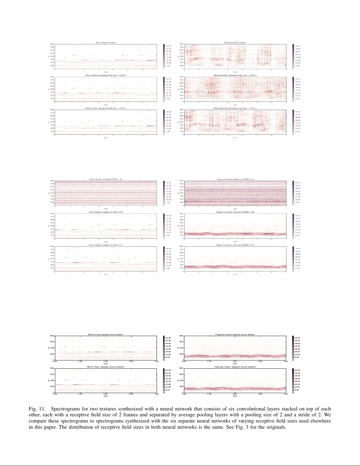
IEEE/A CM TRANSA CTIONS ON A UDIO, SPEECH, AND LANGU A GE PR OCESSING 1 Synthesizing Di v erse, High-Quality Audio T e xtures Joe Antognini, Matt Hof fman, Ron J. W eiss Abstract —T exture synthesis techniques based on match- ing the Gram matrix of feature acti vations in neural networks ha ve achieved spectacular success in the image domain. In this paper we extend these techniques to the audio domain. W e demonstrate that synthesizing diverse audio textures is challenging, and ar gue that this is because audio data is relatively lo w-dimensional. W e theref ore introduce two new terms to the original Grammian loss: an autocorrelation term that pr eserves rhythm, and a diversity term that encourages the optimization procedure to synthesize unique textures. W e quantitatively study the impact of our design choices on the quality of the synthesized audio by introducing an audio analogue to the Inception loss which we term the V GGish loss. W e show that there is a trade-off between the diversity and quality of the synthesized audio using this technique. W e additionally perform a number of experiments to qualitatively study how these design choices impact the quality of the synthesized audio. Finally we describe the implications of these results for the problem of audio style transfer . Index T erms —Machine learning, A udio, T exture synthe- sis I . I N T RO D U C T I O N T exture synthesis has been studied for ov er fifty years [ 1 ]. The problem is to take a sample of some textured data (usually an image) and generate synthesized data which hav e the same texture, b ut are not identical to the original sample. This problem is interesting as a machine learning problem in its o wn right, but successful texture synthesis methods can also elucidate the way in which humans percei ve texture [2]. Portilla and Simoncelli [ 3 ] pioneered a very successful approach to image texture synthesis that tries to find a complete set of statistics that describe the perceptually rele vant aspects of a given texture. T o synthesize a new texture, a random input is perturbed until its statistics match those of the targets. Portilla and Simoncelli [ 3 ] de veloped a set of four classes of statistics consisting of 710 parameters which produced extremely realistic images of natural and synthetic textures. McDermott and Simoncelli [ 2 ] used a similar approach to develop four W ork done as a Google AI Resident classes of statistics in a cochlear model to synthesize textural audio spectrograms. This work produced con- vincing audio data for many natural audio textures (e.g., insects in a swamp, a stream, applause), but had dif ficulty with pitched and rhythmic textures (e.g., wind chimes, walking on gravel, church bells). Gatys et al. [ 4 ] introduced an extremely successful technique that replaced hand-crafted statistics with Gram- matrix statistics derived from the hidden feature acti va- tions of a trained con volutional neural network (CNN). By perturbing a random input to match these Gram matrices, Gatys et al. [ 4 ] produced compelling textures that were far more complicated than those achieved by any earlier work. Gi ven the success of Gatys et al. [ 4 ] in the image domain relativ e to the hand-crafted approach of Portilla and Simoncelli [ 3 ], it is natural to ask whether a similar CNN-based strategy could be adapted to the audio domain to build on the hand-crafted approach of McDermott and Simoncelli [ 2 ]. Ulyanov and Lebedev [ 5 ] proposed just such an extension of the approach of [ 4 ] to audio. Their basic approach works fairly well on many of the 15 examples they consider , but (as we demonstrate in Sec. IV) it has some of the same failure modes as the approach of McDermott and Simoncelli [2]. In this work, we examine the causes of these problems, analyze why they are more serious in the audio domain than in the image domain, and propose techniques to fix them. I I . P R E L I M I N A R I E S A N D A N A LY S I S W e begin by defining a rigorous notion of “audio texture”. Borrowing from Portilla and Simoncelli [ 3 ], we define an audio texture to be an infinitely long stationary random process that follows an exponential- family (maximum-entropy) distribution defined by a set of local sufficient-statistic functions φ that are computed on patches of size M : p λ ( x ) ∝ exp { λ > P ∞ t =0 φ ( x t,...,t + M ) } , E p λ [ φ ] = ¯ φ. (1) W e only ev er observe finite clips from this theoretically infinite signal. If an observed clip is long enough relativ e to M and the dimensionality of φ , then we can reliably estimate the expected sufficient statistics ¯ φ from data. 0000–0000/00$00.00 c  2018 IEEE IEEE/A CM TRANSA CTIONS ON A UDIO, SPEECH, AND LANGUA GE PROCESSING 2 The first practical question we face is whether to model the data in the time domain (i.e., the raw wa veform) or the frequency domain (via a spectrogram). Although direct time-domain modeling has seen enormous success in recent years with W av eNet [ 6 ], these autoregres- si ve techniques are still slow to train and e xtremely computationally demanding at synthesis-time. Follo wing Ulyanov and Lebedev [ 5 ], we instead use the spectrogram representation in this work. This incurs the disadvantage of needing to in vert the spectrogram to recover audio with the Griffin-Lim algorithm [ 7 ], which can introduce artifacts, but is much faster and permits the unsupervised techniques we use in this work, eliminating the need to train a large model. Nai vely , an audio spectrogram can be treated like a two- dimensional greyscale image, with time on one axis and frequency on the other . But in texture synthesis, it is more natural to treat frequency bins in an audio spectrogram as channels (analogous to RGB color channels in an image) rather than spatial dimensions. Audio textures are not stationary on the frequency axis—shifts in frequency tend to change the semantic meaning of a sound. Therefore, although the “spectrogram-as-image” interpretation can work well for some analysis problems [ 8 ], it is a poor fit to the assumptions underlying texture synthesis. T reating spectrograms as one-dimensional multi- channel stationary signals raises an important statistical issue that is not as salient in image texture synthesis. Images typically hav e only three channels, whereas audio spectrograms hav e as many channels as there are samples in the FFT windo w divided by two (typically some power of two between 128 and 2048). Furthermore, the number of patches that are av eraged to estimate the statistics that define the target texture distribution is on the order of the length of the signal, whereas in images the number of patches grows as the product of the dimensions. So in audio texture synthesis, we need to estimate a function of more channels with fe wer observations, which may lead to ov erfitting. W e indeed find that synthesizing di verse audio textures is more dif ficult than synthesizing div erse images and extra care must be taken to encourage di versity (with tongue planted in cheek, this may perhaps be called a curse of low dimensionality). I I I . M E T H O D S A. Signal pr ocessing W e produce audio textures by transforming the target audio to a log spectrogram and synthesizing a new spectrogram. W e then use the Grif fin-Lim algorithm [ 7 ] to in vert the spectrogram and generate the synthesized audio texture. If necessary , we resample the target audio to 16 kHz and normalize. W e produce a spectrogram by taking the absolute value of the short-time Fourier transform with a Hann windo w of size 512 samples and a hop size of 64 samples. Although taking the absolute value removes any explicit phase information, if the hop size is less than or equal to half the windo w size phase information is implicitly retained (i.e., there exists a unique audio signal corresponding to such a spectrogram up to a global phase; [ 9 ]). W e then add 1 to every magnitude in the spectrogram and take the natural logarithm. Adding 1 guarantees that the log-spectrogram is finite and positiv e. B. Arc hitectur e of the neural networks W e obtained the best textures with a set of six single- hidden-layer random CNNs. Unlike the case of image texture synthesis, audio spectrograms are one-dimensional so we therefore use a one-dimensional con volution. Each CNN had a con volutional kernel with a dif ferent width, v arying in powers of 2 from 2 to 64 frames. W e applied a ReLU activ ation after the con volutional layers. Each layer had 512 filters randomly drawn using the Glorot initialization procedure [ 10 ]. Several authors have found that random con volutional layers perform as well as trained con volutional layers for image texture synthesis [ 11 , 12 ]. Shu et al. [ 13 ] furthermore sho wed that a random CNN retains as much information to reconstruct an image as a trained con volutional network, if not more. Although we also tried synthesizing textures with an audio model that was trained on AudioSet [ 14 ], a dataset consisting of about one million 10 second audio clips with 527 labels, we did not find that this trained model produced textures that were any better than those produced by a random CNN. Using an ensemble of CNNs with varying kernel sizes is crucial for obtaining high quality textures since each kernel size is most sensitiv e to audio features whose duration is comparable to the kernel size. The features of real-world audio can span many different timescales (e.g., just a few milliseconds for a clap and up to se veral seconds for a bell) so it is important to use an architecture which is sensiti ve to the range of timescales that is likely to be encountered. W e consider the impact of our architecture design choices experimentally in Section IV -C. C. Loss terms The loss we minimize consists of three terms: L = L Gram + α L autocorr + β L div . (2) The first term, L Gram , was introduced by Gatys et al. [ 4 ] and is intended to capture the av erage local correlations IEEE/A CM TRANSA CTIONS ON A UDIO, SPEECH, AND LANGUA GE PROCESSING 3 between features in the texture. The second term, L autocorr , we adapt from Sendik and Cohen-Or [ 15 ] and is intended to capture rhythm. The final term, L div , we introduce to pre vent the optimization process from exactly copying the original texture. The hyperparameters α and β are used to set the relati ve importance of these three terms. W e find that α = 10 3 and β = 10 − 4 work well for many of the textures we studied, although hyperparameter tuning is sometimes required. In particular, highly rhythmic textures generally require a larger choice of α and a lo wer choice of β . 1) Gram loss: Let us write the features of the k th con volutional network as F k tµ , where t indicates the position of a patch in the feature map (i.e., the time in the spectrogram), and µ indicates the filter . The Gram matrix for the k th conv olutional network is the time- av eraged outer product between the k th feature map with itself: G k µν = 1 T X t F k tµ F k tν , (3) where T is the number of windows in the spectrogram W e match this statistic by minimizing the Frobenius norm of the difference between the Gram matrices of the synthesized texture and the target for all layers and normalizing to the Frobenius norm of the target texture Gram matrix: L Gram = P k,µ,ν ( G k µν − e G k µν ) 2 P k,µ,ν ( e G k µν ) 2 . (4) Throughout this paper tilde denotes the target texture. 2) A utocorr elation loss: While minimizing the Gram loss alone produces excellent audio for many kinds of audio textures, we sho w in Sec. IV -B 1 that the Gram loss fails to capture rhythm. T o this end, we adapt a loss term introduced by Sendik and Cohen-Or [ 15 ] deriv ed from the autocorrelation of the feature maps that was de veloped to capture periodic structure in image textures. 1 The autocorrelation of the k th feature map is A k τ µ = F − 1 f h F t [ F k tµ ] F t [ F k tµ ] ∗ i , (5) where F t represents the discrete Fourier transform with respect to time t , ∗ represents complex conjugation, and τ represents the lag. The autocorrelation loss is the sum of the normalized Frobenius norms of the squared differences between the target and synthesized autocorrelation maps: L autocorr = P k,τ ,µ ( A k τ µ − e A k τ µ ) 2 P k,τ ,µ ( e A k τ µ ) 2 . (6) 1 Note that Sendik and Cohen-Or [ 15 ] use a v ariant of the feature map autocorrelation called the structural matrix, but we find that the autocorrelation works well and is faster to compute. W e generally do not expect to encounter rhythmic structure on timescales longer than a fe w seconds, and autocorrelations on extremely short timescales (under 200 ms) are captured within the receptiv e fields of indi vidual networks. Including very short and long lags in the loss tends to encourage ov erfitting without adding any useful rhythmic acti vity to the texture (this is particularly true for lags near 0 since the autocorrelation will always be largest there and will therefore be the largest contributor to L autocorr ). For this reason we only sum over lags of 200 ms to 2 s. 3) Diversity loss: As we show in Sec. IV -B 2, a do wnside of using the pre vious two loss terms alone is that they tend to reproduce the original texture exactly . Sendik and Cohen-Or [ 15 ] proposed a diversity term for image texture synthesis of the form L Sendik = − P k,t,µ  F k tµ − e F k tµ  2 , (7) which is maximized when the two feature maps match exactly . W e found that this div ersity term has two short- comings: first, because this term can become arbitrarily negati ve, it can dominate the total loss and destabilize the optimization (see Fig. 1); second, we find that this loss has a tendency to reproduce the original input, but slightly shifted in time (see Fig. 2). T o address these two issues, we propose the following shift-in variant div ersity term: L div = max s  P k,t,µ ( e F k tµ ) 2 P k,t,µ ( F k t + s,µ − e F k tµ ) 2  , (8) where the shift s can take on values ranging from 0 to T − 1 . In other words, we compute the negati ve inv erse of the div ersity term of Eq. 7 for all possible relative shifts between the original and synthesized textures and then take the maximum. Since computing this loss for all possible shifts is computationally expensi ve, we compute this loss in steps of 50 frames, cycling through different sets of frames in each step of the optimization process, along with computing the loss for the shifts which yielded the largest loss in the last 10 optimization steps. D. Optimization W e find that L-BFGS-B [ 16 ] works well to minimize the loss and obtain high quality audio textures. W e optimized for 2000 iterations and used 500 iterations of the Griffi n-Lim algorithm. W e furthermore found it useful to include the div ersity loss term for only the first 100 iterations; by this point the optimizer had found a nontri vial local optimum, and continuing to incorporate the diversity loss reduced texture quality . Spectrograms of four synthesized textures are sho wn in Fig. 3. W e sho w the IEEE/A CM TRANSA CTIONS ON A UDIO, SPEECH, AND LANGUA GE PROCESSING 4 0 1 0 0 2 0 0 3 0 0 4 0 0 5 0 0 6 0 0 S t e p − 0 . 0 0 2 0 . 0 0 0 0 . 0 0 2 0 . 0 0 4 0 . 0 0 6 0 . 0 0 8 0 . 0 1 0 L o ss 0 1 0 0 2 0 0 3 0 0 4 0 0 5 0 0 6 0 0 S t e p − 1 . 0 − 0 . 5 0 . 0 0 . 5 1 . 0 1 . 5 2 . 0 2 . 5 3 . 0 3 . 5 L G r am / L 0 1 0 0 2 0 0 3 0 0 4 0 0 5 0 0 6 0 0 S t e p − 2 0 − 1 0 0 1 0 2 0 3 0 4 0 5 0 6 0 L au t oc or r e l at i on / L 0 1 0 0 2 0 0 3 0 0 4 0 0 5 0 0 6 0 0 S t e p − 6 0 − 5 0 − 4 0 − 3 0 − 2 0 − 1 0 0 1 0 2 0 L S e n d i k / L Fig. 1. The ov erall loss and the relativ e contributions of the three components during optimization of a wind chimes texture using L Sendik instead of L div . This diversity term can lead to negativ e losses, which in turn makes optimization difficult when the loss passes through zero. In part to av oid these instabilities we propose a div ersity term of the form Eq. 8. 0 1 2 3 4 5 6 7 S h i f t b e t w e e n o r i g i n a l a n d sy n t h e si z e d sp e c t r o g r a m ( s) 1 0 - 1 1 0 0 1 0 1 1 0 2 − 1 / L S e n d i k 4 . 9 2 4 . 9 6 5 . 0 0 5 . 0 4 1 0 - 1 1 0 0 1 0 1 1 0 2 Fig. 2. The inv erse negati ve diversity term used by Sendik and Cohen-Or [ 15 ] as a function of a synthesized texture shifted in time. The synthesized texture closely matches the original texture, but is shifted in time by about five seconds. L Sendik fails to capture this effect as demonstrated by the sharp peak. Inset zooms in on the peak to show that the peak is resolved. relati ve values of the various loss terms during optimiza- tion in Fig. 4. Corresponding audio for all spectrograms, along with supplementary information, can be found at https://antognini- google.github.io/audio textures/. I V . E X P E R I M E N T S A. Quantitative evaluation of textur e quality Quantitati vely ev aluating the quality of generati ve models is difficult. Salimans [ 17 ] dev eloped a useful quantitati ve metric for comparing generativ e adversarial networks based on the Kullback-Liebler div ergence of the label predictions giv en by the Inception classifier [ 18 ] between the sampled images and the original dataset. W e adapt this “Inception score” to assess the quality of our audio textures compared to other methods. Rather than Inception, we use the “VGGish” CNN 2 that was trained on AudioSet. 3 The motiv ation for our “VGGish score” is that the label predictions produced by the VGGish model should match between the original and synthesized textures. T o this end, we define the score as S VGGish ≡ exp [ E x [ KL ( p VGGish ( y | e x ) || p VGGish ( y | x ))]] , (9) where y represents the VGGish label predictions and x represents the texture audio. W e compute S VGGish ov er the 168 textures used by McDermott and Simoncelli [ 2 ]. These textures span a broad range of sound, including natural and artificial sounds, pitched and non-pitched sounds, and rhythmic and non-rhythmic sounds. W e com- pare this VGGish score between our models optimized with different loss terms and the approaches used by Ulyanov and Lebedev [ 5 ] and McDermott and Simoncelli [ 2 ] in T able I, separating out the scores for pitched and rhythmic textures. W e also compare an autocorrelation score and a div ersity score computed from the generated spectrograms discussed in Sections IV -B 1 and IV -B 2, respecti vely . The best VGGish scores are obtained by using L Gram alone. As expected, adding L autocorr substantially reduces the autocorrelation score, though at the cost of increasing the diversity score, and adding a larger weight to L div generally reduces the di versity score. The lo west di versity scores are obtained by McDermott and Simoncelli [ 2 ], though at the cost of substantially higher autocorrelation scores and relativ ely large VGGish scores for pitched textures. It is unsurprising that adding L div reduces the VGGish score because introducing any div ersity will generally reduce the VGGish score (the model could achiev e a perfect VGGish score simply by copying the original input). It is, howe ver , surprising that adding L autocorr alone also reduces the VGGish score. Although introducing L autocorr qualitati vely seems to increase overfitting, this ov erfitting occurs on very long timescales (i.e., the model will reproduce sev eral seconds that sound very similar to the original audio). Introducing L autocorr seems to make the optimization process more dif ficult for timescales much shorter than the minimum lag considered by L autocorr , which leads to lower quality on short timescales and thus higher VGGish scores. 2 A v ailable from https://github.com/tensorflo w/models/tree/master/ research/audioset. 3 VGGish produces 128 dimensional embeddings rather than label predictions. T o obtain label predictions we trained a set of 527 logistic regression classifiers on top of the AudioSet embeddings (AudioSet’ s 527 classes are not mutually exclusi ve.) W e trained for 100,000 steps with a learning rate of 0.1 and achiev ed a test accuracy of 99.42% and a test cross entropy loss of 0.0584. IEEE/A CM TRANSA CTIONS ON A UDIO, SPEECH, AND LANGUA GE PROCESSING 5 Fig. 3. Four pairs of synthesized audio textures with the originals. These textures include pitched audio (wind chimes, upper right), rhythmic audio (tapping, upper left), speech (lo wer left), and natural sounds (lo wer right). T ABLE I A C O M PA R I S O N O F S C O R E S B E T W E E N O U R M O D E L A N D O T H E R W O R K . VGGish ( × 10 − 4 ) Autocorrelation Div ersity Rthm. Ptch. Other Rthm. Ptch. Other Rthm. Ptch. Other Spectrograms recovered via Griffin-Lim 9.7 12.6 7.1 7.4 0.54 2.9 21.4 29.7 22.7 McDermott and Simoncelli [2] 16.7 33.2 8.3 542.0 408.1 421.9 1.6 1.6 2.0 Ulyanov and Lebedev [5] 13.4 26.8 10.0 40.6 23.3 27.4 2.9 3.0 3.3 L Gram 9.9 16.8 7.3 29.0 9.7 6.5 2.4 3.0 3.5 L Gram + L autocorr 17.8 21.3 17.9 13.3 7.4 15.6 3.4 5.4 5.0 L Gram + L autocorr + L div ( β = 10 − 5 ) 14.5 23.0 12.2 13.0 2.3 7.2 3.8 6.8 4.4 L Gram + L autocorr + L div ( β = 10 − 3 ) 14.9 19.0 10.0 4.7 3.7 7.1 5.0 4.9 3.9 1 0 0 1 0 1 1 0 2 1 0 3 S t e p s 1 0 0 1 0 1 1 0 2 1 0 3 1 0 4 1 0 5 1 0 6 1 0 7 1 0 8 L o ss 1 0 0 1 0 1 1 0 2 1 0 3 S t e p s 0 . 0 0 . 2 0 . 4 0 . 6 0 . 8 1 . 0 F r a c t i o n o f t o t a l l o ss G r a m a u t o c o r r e l a t i o n d i v e r si t y Fig. 4. Left panel: loss during optimization of the wind chimes texture. Right panel: the fraction of the total loss each of the three terms contributes during optimization. B. Effect of the differ ent loss terms 1) A utocorr elation loss: T o demonstrate the necessity of L autocorr we synthesize textures with a variety of v alues of α . For simplicity we set β = 0 in these experiments (i.e., we exclude L div from the total loss). W e show spectrograms for a highly rhythmic tapping texture using two different values of α in Fig. 5. If the weight of L autocorr is small, the synthesized textures reproduce tapping sounds which lack the precise rhythm of the original. Only when α is sufficiently large is the rhythm reproduced. W e further demonstrate that minimizing L autocorr reproduces rhythms by showing in Fig. 6 the autocorrelation functions of the spectrograms of a rhythmic and non-rhythmic texture. 4 W e furthermore compute the squared loss between the autocorrelation of each synthesized texture and its target texture, normalized to the Frobenius norm of the autocorrelation of the target texture. W e present these scores in T able I. Qualitativ ely we find that, as expected, L autocorr is most important in textures with substantial rhythmic activity and so it is useful to use a relatively large value for α for these rhythms. F or te xtures without substantial rh ythmic acti vity we find that a smaller choice of α produces higher quality 4 Note that this is not directly minimized by minimizing Eq. 6 which is a function of the CNN features, not the spectrogram itself. IEEE/A CM TRANSA CTIONS ON A UDIO, SPEECH, AND LANGUA GE PROCESSING 6 Fig. 5. Spectrograms of a rhythmic tapping texture synthesized with different weights for L autocorr . Rhythm is only reproduced when the weight on L autocorr is sufficiently large. textures. 2) Diversity loss: T o demonstrate the effect of L div we synthesize textures with a v ariety of values of β , keeping α fixed to 10 3 . W e show in Fig. 7 spectrograms synthesized with two different values of β for two highly structured textures: wind chimes and speech. Smaller v alues of β generally reproduce the original texture but shifted in time (about 2 s for the wind chimes and about 3.25 s for speech). Larger values of β produce spectrograms which are not simple translations of the original input, but the quality of the resulting audio is much lower . In the case of the wind chimes the chimes do not have the hard onset in the original, and in the case of speech the voice is echoey and superimposes dif ferent phonemes. This is an instance of a more general di versity-quality trade-off in texture synthesis. In Fig. 8 we sho w the VGGish score (a rough proxy for texture quality) vs. the weight on the div ersity term. As the weight on the div ersity term increases, the average quality decreases. W e furthermore calculate the div ersity loss on the spectrograms themselves to get a div ersity score and present these scores in T able I. W e find that it is crucial to tune the loss weights for dif ferent texture classes in order to obtain the highest quality textures. Large α and large β , for example, is especially important for reliably generating rhythmic textures. Pitched audio generally requries a smaller choice of α and β . For non-textured audio like speech and music, high quality audio is only obtained with a large α and small β , which will only reproduce the original with some shift; since these kinds of audio do not obey the assumptions set out in Section II, any set of weights that does not reproduce the original will produce low quality audio. C. Neural network arc hitecture The receptive field size of the con volutional kernel has a strong ef fect on the quality and div ersity of the synthesized textures. W e show in Fig. 9 the effe ct of changing the receptiv e field size for two textures. T o do this, we use the same set of single layer CNNs with exponentially increasing kernel sizes, but varying the maximum kernel size from 2 frames to 8. CNNs with very small receptive fields produce nov el, but poor -quality textures that fail to capture long- range structure. Networks with large receptive fields tend to reproduce the original. This is an example of the quality-di versity trade-off in texture synthesis. Another design choice we consider is the number of filters in the each network. W e sho w in Fig. 10 the results of using 32, 128, and 512 filters to synthesize two te xtures. Note that because there are six CNNs in all with varying kernel sizes, the total number of activ ations varies from 192 to 3072. At least 128 filters are necessary to get reasonable textures, but the quality continues to improve with 512 filters. W e considered stacking six con volutional layers on top of each other, each with a receptiv e field of 2 and separated by an average pooling layer with a pool size of 2 and a stride of 2. This network has the same distribution of recepti ve field sizes as the six separate networks, but the input to each layer here must pass through the (random) filters of all the earlier layers. W e compare spectrograms generated with this network to the six separate networks that we use else where in Fig. 11. The only effect of stacking the layers is a modest degradation in the quality of long-range sounds, best seen in the wind chimes texture. V . D I S C U S S I O N A. T owards compelling audio style transfer After Gatys et al. [ 4 ] dev eloped the Gram-based approach for texture synthesis, a natural extension was to propose a similar technique for artistic style transfer [ 19 ] in which there is an additional content term in the loss which is minimized by matching the high-lev el features of a second image. There hav e now been a variety of impressi ve results for image style transfer [ 20 , 21 , 22 ]. There hav e been a few attempts to extend these techniques to audio style transfer [ 5 , 23 , 24 ], and while the results are plausible, they are underwhelming compared to the results in the image domain. What makes the audio domain so much more challenging? The first issue is that it is unclear what is meant by “style transfer . ” The simplest form of style transfer would be to take a melody played on one instrument and make it sound as though it were played on another; or similarly voice con version, i.e., taking audio spoken by one person and making it sound as though it had been IEEE/A CM TRANSA CTIONS ON A UDIO, SPEECH, AND LANGUA GE PROCESSING 7 0 1 2 3 4 5 6 7 L a g ( s) 0 5 0 0 1 0 0 0 1 5 0 0 2 0 0 0 2 5 0 0 3 0 0 0 A u t o c o r r e l a t i o n m a g n i t u d e O r i g i n a l : T a p p i n g 1 - 2 - 3 0 1 2 3 4 5 6 7 L a g ( s) 0 5 0 0 1 0 0 0 1 5 0 0 2 0 0 0 2 5 0 0 3 0 0 0 A u t o c o r r e l a t i o n m a g n i t u d e S y n t h e t i c : T a p p i n g 1 - 2 - 3 , a u t o c o r r e l a t i o n w e i g h t 0 0 1 2 3 4 5 6 7 L a g ( s) 0 5 0 0 1 0 0 0 1 5 0 0 2 0 0 0 2 5 0 0 3 0 0 0 A u t o c o r r e l a t i o n m a g n i t u d e S y n t h e t i c : T a p p i n g 1 - 2 - 3 , a u t o c o r r e l a t i o n w e i g h t 1 0 0 0 0 0 0 1 2 3 4 5 6 7 L a g ( s) 5 2 0 0 5 4 0 0 5 6 0 0 5 8 0 0 6 0 0 0 A u t o c o r r e l a t i o n m a g n i t u d e O r i g i n a l : B l e n d e r 0 1 2 3 4 5 6 7 L a g ( s) 5 2 0 0 5 4 0 0 5 6 0 0 5 8 0 0 6 0 0 0 6 2 0 0 A u t o c o r r e l a t i o n m a g n i t u d e S y n t h e t i c : B l e n d e r , a u t o c o r r e l a t i o n w e i g h t 0 0 1 2 3 4 5 6 7 L a g ( s) 5 2 0 0 5 4 0 0 5 6 0 0 5 8 0 0 6 0 0 0 6 2 0 0 A u t o c o r r e l a t i o n m a g n i t u d e S y n t h e t i c : B l e n d e r , a u t o c o r r e l a t i o n w e i g h t 1 0 0 0 0 0 Fig. 6. Autocorrelation functions of a rhythmic (top ro w) and non-rhythmic (bottom row) texture for the original (left column) and two weights on L autocorr . Whereas the non-rhythmic texture has a flat autocorrelation function, the autocorrelation function of the rhythmic texture displays structure that is reproduced only when the weight on L autocorr is large. Fig. 7. Spectrograms synthesized with different weights β on L div for two non-stationary sounds: wind chimes (left) and speech (right). 1 0 - 1 0 1 0 - 9 1 0 - 8 1 0 - 7 1 0 - 6 1 0 - 5 1 0 - 4 1 0 - 3 1 0 - 2 1 0 - 1 1 0 0 Di v e r si t y w e i g h t 0 . 0 0 1 0 0 . 0 0 1 2 0 . 0 0 1 4 0 . 0 0 1 6 0 . 0 0 1 8 0 . 0 0 2 0 V G G i sh sc o r e Fig. 8. The diversity-quality trade-off in texture synthesis. The VGGish score is a rough proxy for texture quality , with lower scores representing higher quality textures. As the diversity weight increases, the av erage quality of the textures decreases. spoken by another [ 25 ]. While this simpler version of style transfer is still an open problem, the more interesting and far more difficult form of style transfer would be taking a melody from one genre (e.g., a Mozart aria) and transforming it into one from another (e.g., a jazz song) by keeping the broad lyric and melodic structure, but replacing the instrumentation, ornamentation, rhythmic patterns, etc., characteristic of one genre with those of another . It is plausible that the simpler form of style transfer can be accomplished with careful design choices in the con volutional architecture [ 25 ]. But it does not appear that such an approach can work for the more complicated kind of style transfer . T o understand why , it is worth comparing the features learned by deep CNNs trained on image vs. audio data. In the image domain there is a well defined feature hierarchy , with lower layers learning simple visual patterns like lines and corners, and later layers learning progressiv ely more complicated and abstract features like dog faces and automobiles in the final layers [ 26 ]. By contrast, CNNs in the audio domain have been far less studied. IEEE/A CM TRANSA CTIONS ON A UDIO, SPEECH, AND LANGUA GE PROCESSING 8 Fig. 9. Spectrograms synthesized from conv olutional networks with different maximum receptive field sizes. Fig. 10. Spectrograms for two textures synthesized with varying numbers of filters in the con volutional layers. W ith 32 filters, the textures hav e isolated power in some frequencies and not others, but hav e not dev eloped any temporal structure. It is not until there are 128 filters that the textures introduce sounds that vary over time. Ho wev er, for complex textures like wind chimes, only 512 filters are suf ficient to produce the hard onsets of bells. See Fig. 3 for the originals. 0 . 0 0 s 1 . 7 5 s 3 . 5 0 s 5 . 2 5 s 7 . 0 0 s T i m e 0 2 0 0 0 4 0 0 0 6 0 0 0 8 0 0 0 Hz W i n d c h i m e s , s t a c k e d n e u r a l n e t w o r k + 8 d B + 1 6 d B + 2 4 d B + 3 2 d B + 4 0 d B + 4 8 d B + 5 6 d B + 6 4 d B 0 . 0 0 s 1 . 7 5 s 3 . 5 0 s 5 . 2 5 s 7 . 0 0 s T i m e 0 2 0 0 0 4 0 0 0 6 0 0 0 8 0 0 0 Hz W i n d c h i m e s , s e p a r a t e n e u r a l n e t w o r k s + 8 d B + 1 6 d B + 2 4 d B + 3 2 d B + 4 0 d B + 4 8 d B + 5 6 d B + 6 4 d B 0 . 0 0 s 1 . 7 5 s 3 . 5 0 s 5 . 2 5 s 7 . 0 0 s T i m e 0 2 0 0 0 4 0 0 0 6 0 0 0 8 0 0 0 Hz F r o g s a n d i n s e c t s , s t a c k e d n e u r a l n e t w o r k + 8 d B + 1 6 d B + 2 4 d B + 3 2 d B + 4 0 d B + 4 8 d B + 5 6 d B + 6 4 d B 0 . 0 0 s 1 . 7 5 s 3 . 5 0 s 5 . 2 5 s 7 . 0 0 s T i m e 0 2 0 0 0 4 0 0 0 6 0 0 0 8 0 0 0 Hz F r o g s a n d i n s e c t s , s e p a r a t e n e u r a l n e t w o r k s + 8 d B + 1 6 d B + 2 4 d B + 3 2 d B + 4 0 d B + 4 8 d B + 5 6 d B + 6 4 d B Fig. 11. Spectrograms for two textures synthesized with a neural network that consists of six con volutional layers stacked on top of each other , each with a recepti ve field size of 2 frames and separated by av erage pooling layers with a pooling size of 2 and a stride of 2. W e compare these spectrograms to spectrograms synthesized with the six separate neural networks of v arying receptiv e field sizes used elsewhere in this paper . The distribution of receptive field sizes in both neural networks is the same. See Fig. 3 for the originals. IEEE/A CM TRANSA CTIONS ON A UDIO, SPEECH, AND LANGUA GE PROCESSING 9 Dieleman [ 27 ] analyzed patterns in the feature activ ations of a deep CNN trained on one million songs from the Spotify corpus in v an den Oord [ 28 ]. Dieleman [ 27 ] found that features in lower layers identified local stylistic and melodic features, e.g., vibrato singing, vocal thirds, and bass drum. Features in later layers identified specific genres, e.g., Christian rock and Chinese pop. Whereas in the image domain the feature activ ations of the higher layers represent the content of the image (e.g., there is a dog in the lower left corner), in the audio domain the later layers instead represent the ov erall style. These dif ferences reflect the way that these CNNs are trained. In the image domain, CNNs are explicitly trained to identify the content of the image. In the audio domain the CNN is instead trained to identify the overall style. This poses a challenge for style transfer because the “content” of the audio consists of the melody and lyrics, but the CNN is nev er trained to identify the content and so it either gets mixed in with other low-le vel textural features or is not propagated to later layers at all. Successful audio style transfer will require a network that can separate the melodic content of audio from its stylistic content the way that image classification CNNs can. The path forward may instead lie with neural networks trained on transcription or Query by Singing/Humming tasks. V I . C O N C L U S I O N S W e hav e demonstrated that the approach to texture synthesis described by Gatys et al. [ 4 ] of matching Gram matrices from con volutional networks can be extended to the problem of synthesizing audio textures. There are, ho wev er, certain differences in the audio domain vs. the image domain that require the addition of two more loss terms to produce div erse, robust audio textures: an autocorrelation term to preserve rhythm, and a div ersity term to encourage the synthesized textures to not exactly reproduce the original texture. W e test our technique across sev eral classes of textures like rhythmic and pitched audio and find that tuning the weights on the autocorrelation and diversity terms is crucial to obtaining the highest quality textures for different classes. The choice of architecture is also important to obtain high quality te xtures; an ensemble random con volutional neural networks with a wide range of receptiv e field sizes allows the model to capture features that occur on timescales across many orders of magnitude. Finally , we show that this method has a trade-off between the div ersity and the quality of the results. A C K N O W L E D G M E N T S The authors are grateful to Josh McDermott for providing the synthesized textures using the technique of McDermott and Simoncelli [ 2 ] for comparison with the technique in this paper . The authors thank Rif A. Saurous for helpful comments on the manuscript. R E F E R E N C E S [1] B. Julesz, “V isual pattern discrimination, ” IRE T ransactions on Information Theory , vol. 8, no. 2, pp. 84–92, 1962. [2] J. H. McDermott and E. P . Simoncelli, “Sound texture perception via statistics of the auditory periphery: evidence from sound synthesis, ” Neur on , vol. 71, no. 5, pp. 926–940, 2011. [3] J. Portilla and E. P . Simoncelli, “ A parametric texture model based on joint statistics of complex wa velet coefficients, ” International Journal of Com- puter V ision , vol. 40, no. 1, pp. 49–70, 2000. [4] L. Gatys, A. S. Ecker , and M. Bethge, “T exture synthesis using conv olutional neural networks, ” in Advances in Neural Information Pr ocessing Systems , 2015, pp. 262–270. [5] D. Ulyanov and V . Lebede v , “ Audio texture synthesis and style transfer , ” 2016. [Online]. A v ailable: https://dmitryulyanov .github .io/ audio- texture- synthesis- and- style- transfer/ [6] A. v . d. Oord, S. Dieleman, H. Zen, K. Si- monyan, O. V inyals, A. Grav es, N. Kalchbrenner , A. Senior , and K. Ka vukcuoglu, “W av eNet: A generati ve model for raw audio, ” arXiv pr eprint arXiv:1609.03499 , 2016. [7] D. Grif fin and J. Lim, “Signal estimation from modified short-time fourier transform, ” IEEE T rans- actions on Acoustics, Speech, and Signal Pr ocessing , vol. 32, no. 2, pp. 236–243, 1984. [8] S. Hershey , S. Chaudhuri, D. P . W . Ellis, J. F . Gemmeke, A. Jansen, R. C. Moore, M. Plakal, D. Platt, R. A. Saurous, B. Seybold, M. Slaney , R. J. W eiss, and K. W ilson, “CNN architectures for large-scale audio classification, ” in IEEE ICASSP , Mar . 2017. [9] N. Sturmel and L. Daudet, “Signal reconstruction from STFT magnitude: A state of the art, ” in International Confer ence on Digital Audio Effects , 2011. [10] X. Glorot and Y . Bengio, “Understanding the dif fi- culty of training deep feedforward neural networks, ” in Pr oceedings of the Thirteenth International Con- fer ence on Artificial Intelligence and Statistics , 2010, pp. 249–256. [11] K. He, Y . W ang, and J. Hopcroft, “ A powerful generati ve model using random weights for the deep image representation, ” in Advances in Neural Information Pr ocessing Systems , 2016, pp. 631–639. IEEE/A CM TRANSA CTIONS ON A UDIO, SPEECH, AND LANGUA GE PROCESSING 10 [12] I. Ustyuzhaninov , W . Brendel, L. A. Gatys, and M. Bethge, “T exture synthesis using shallow con- volutional networks with random filters, ” arXiv pr eprint arXiv:1606.00021 , 2016. [13] Y . Shu, M. Zhu, K. He, J. Hopcroft, and P . Zhou, “Understanding deep representations through random weights, ” arXiv pr eprint arXiv:1704.00330 , 2017. [14] J. F . Gemmeke, D. P . Ellis, D. Freedman, A. Jansen, W . Lawrence, R. C. Moore, M. Plakal, and M. Ritter , “ Audio set: An ontology and human-labeled dataset for audio ev ents, ” in IEEE ICASSP , 2017. [15] O. Sendik and D. Cohen-Or , “Deep correlations for texture synthesis, ” ACM T ransactions on Graphics (TOG) , vol. 36, no. 5, p. 161, 2017. [16] C. Zhu, R. H. Byrd, P . Lu, and J. Nocedal, “ Al- gorithm 778: L-BFGS-B: Fortran subroutines for large-scale bound-constrained optimization, ” ACM T ransactions on Mathematical Softwar e (TOMS) , vol. 23, no. 4, pp. 550–560, 1997. [17] T . Salimans, I. Goodfellow , W . Zaremba, V . Cheung, A. Radford, and X. Chen, “Improved techniques for training GANs, ” in Advances in Neural Information Pr ocessing Systems , 2016, pp. 2234–2242. [18] C. Szegedy , W . Liu, Y . Jia, P . Sermanet, S. Reed, D. Anguelov , D. Erhan, V . V anhoucke, A. Rabi- novich et al. , “Going deeper with con volutions, ” in CVPR , 2015. [19] L. A. Gatys, A. S. Ecker , and M. Bethge, “ A neural algorithm of artistic style, ” arXiv preprint arXiv:1508.06576 , 2015. [20] T . Q. Chen and M. Schmidt, “Fast Patch-based Style T ransfer of Arbitrary Style, ” ArXiv e-prints , Dec. 2016. [21] V . Dumoulin, J. Shlens, M. Kudlur , A. Behboodi, F . Lemic, A. W olisz, M. Molinaro, C. Hirche, M. Hayashi, E. Bagan et al. , “ A learned rep- resentation for artistic style, ” arXiv preprint arXiv:1610.07629 , 2016. [22] D. Ulyanov , V . Lebedev , A. V edaldi, and V . S. Lem- pitsky , “T exture networks: Feed-forward synthesis of textures and stylized images. ” in ICML , 2016, pp. 1349–1357. [23] E. Grinstein, N. Duong, A. Ozero v , and P . Perez, “ Audio style transfer , ” arXiv preprint arXiv:1710.11385 , 2017. [24] S. Barry and Y . Kim, ““Style” transfer for musical audio using multiple time-frequency representations, ” 2018. [Online]. A v ailable: https: //openre view .net/forum?id=BybQ7zWCb [25] J. Choro wski, R. J. W eiss, R. A. Saurous, and S. Bengio, “On using backpropagation for speech texture generation and voice conv ersion, ” arXiv pr eprint arXiv:1712.08363 , 2017. [26] C. Olah, A. Mordvintsev , and L. Schubert, “Feature visualization, ” Distill , vol. 2, no. 11, p. e7, 2017. [27] S. Dieleman, “Recommending music on spotify with deep learning, ” 2014. [Online]. A v ailable: http: //benanne.github .io/2014/08/05/spotify- cnns.html [28] A. V an den Oord, S. Dieleman, and B. Schrauwen, “Deep content-based music recommendation, ” in Advances in Neural Information Pr ocessing Systems , 2013, pp. 2643–2651. Joseph M. Antognini is a Google AI resident. At Google he has worked on applying machine learning to audio synthesis and studying the foundations of machine learning. He receiv ed his Ph.D. in astronomy from The Ohio State Univ ersity in 2016. Matthew D. Hoffman is a senior research scientist at Google. His main research focus is in probabilistic modeling and approximate inference algorithms. He has worked on vari- ous applications including music information retriev al, speech enhancement, topic modeling, learning to rank, computer vision, user inter- faces, user behavior modeling, social network analysis, digital imaging, and astronomy . He is a co-creator of the widely used statistical modeling package Stan. Ron J. W eiss is a software engineer at Google where he has worked on content-based audio analysis, recommender systems for music, and noise robust speech recognition. Ron com- pleted his Ph.D. in electrical engineering from Columbia University in 2009 where he worked in the Laboratory for the Recognition of Speech and Audio. From 2009 to 2010 he was a postdoctoral researcher in the Music and Audio Research Laboratory at Ne w Y ork Uni versity .