Travel time tomography with adaptive dictionaries
We develop a 2D travel time tomography method which regularizes the inversion by modeling groups of slowness pixels from discrete slowness maps, called patches, as sparse linear combinations of atoms from a dictionary. We propose to use dictionary le…
Authors: Michael Bianco, Peter Gerstoft
1 T ra v el time tomography with adapti ve dictionaries Michael Bianco, Student Member , IEEE, Peter Gerstoft, Member , IEEE, Abstract —W e develop a 2D travel time tomography method which regularizes the in version by modeling gr oups of slowness pixels from discr ete slowness maps, called patches, as sparse linear combinations of atoms from a dictionary . W e propose to use dictionary learning during the inv ersion to adapt dictionaries to specific slowness maps. This patch regularization, called the local model, is integrated into the overall slowness map, called the global model. The local model considers small-scale v ariations using a sparsity constraint and the global model considers larger - scale features constrained using ` 2 regularization. This strategy in a locally-sparse trav el time tomography (LST) approach enables simultaneous modeling of smooth and discontinuous slowness features. This is in contrast to conventional tomography methods, which constrain models to be exclusively smooth or discontinuous. W e develop a maximum a posteriori formulation for LST and exploit the sparsity of slowness patches using dictionary learning. The LST approach compares fav orably with smoothness and total v ariation regularization methods on densely , but irregularly sampled synthetic slowness maps. Index T erms —Dictionary learning, machine learning, inverse problems, geophysics, seismology , sparse modeling I . I N T RO D U C T I O N T ravel time tomography methods estimate Earth slowness structure, which contains smooth and discontinuous features at multiple spatial scales, from tra vel times of seismic waves between recording stations. The estimation of slowness (in- verse of speed) models from trav el times is often formulated as a discrete linear in verse problem, where the perturbations in trav el time relati ve to a reference are used to infer the unkno wn structure [1], [2]. Such problems are ill-posed, with irregular ray coverage of en vironments, and require regularization to obtain physically plausible solutions. W e propose a 2D travel time tomography method which regularizes the in version by assuming small groups of slo wness pixels from a discrete slo wness map, called patches, are well approximated by sparse linear combinations of atoms from a dictionary . In this sparse model [3], [4], the atoms represent elemental slowness patches and can be generic dictionar- ies, e.g. wa velets, or adapted to specific data by dictionary learning [5], [6]. This patch regularization, called the local model, is integrated into the o verall slo wness map, called the global model. Whereas the local model considers small- scale variations using a sparsity constraint, the global model considers larger -scale features which are constrained using ` 2 regularization. This local-global modeling strategy with dictionary learning has been successful in image denoising [3], [7], [8] and inpainting [9], where natural image content is recovered from M. Bianco and P . Gerstoft are with the Scripps Institution of Oceanog- raphy , University of California San Diego, La Jolla, CA 92093-0238, USA, http://noiselab .ucsd.edu (e-mail: mbianco@ucsd.edu; gerstoft@ucsd.edu) Supported by the Office of Nav al Research, Grant No. N00014-18-1-2118. noisy or incomplete data. W e use this strategy to recov er true slowness fields from travel time tomograph y by simultane- ously modeling smooth and discontinuous slo wness features. This gives an improv ement over con ventional methods with global damping and smoothness regularization [2], [10] and pixel level regularization e.g. total variation (TV) regulariza- tion [11], [12] which regularize tomography by encouraging smooth or discontinuous slownesses. Relativ e to existing to- mography methods based on wa velets [13], [14] and sparse dictionaries [15]–[18], our formulation of the tomography problem permits the adaptation of the sparse dictionaries to trav el time data and ray sampling by dictionary learning tech- niques, for which many methods exist [3], [5], [6], [8], [19]. Sparse reconstruction performance is often improv ed using adaptiv e dictionaries, which represent well specific data, over generic dictionaries which achieve acceptable performance for many tasks [4]. Sparse modeling assumes signals can be reconstructed to acceptable accuracy using few or sparse vectors, called atoms , from a potentially large set or dictionary of atoms. The parsimony of sparse representations [4] often provides better regularization than, for example, traditional ` 2 model damp- ing [2]. Early sparse approaches were dev eloped in seismic decon volution [20], [21]. This philosophy has since become ubiquitous in signal processing for image and video denoising [3], [7], [8] and inpainting [9], and medical imaging [22], [23], to name a fe w examples. Recent works in acoustics and seismics have utilized sparse modeling, e.g. beamforming [24], [25], matched field processing [26], estimation of ocean acoustic properties [27]–[32]. Dictionary learning has been used to denoise seismic [33], [34] and ocean acoustic [27] recordings, to regularize full waveform in version [35], [36], and to regularize ocean sound speed profile in version [28], [29]. Inspired by image denoising [7], we develop a sparse and adaptiv e 2D trav el time tomography method, which we refer to as locally-sparse trav el time tomography (LST). Whereas in [7], the image pixel values are directly observed, in LST the pixel v alues are inferred from measurements [23]. This necessitates an extra term to fit slowness pixels to travel time observations. W e dev elop a maximum a posteriori (MAP) formulation for LST and use the iterati ve thresholding and signed K-means (ITKM) [6] dictionary learning algorithm to design adaptiv e dictionaries. This improves slowness models ov er generic dictionaries. W e demonstrate the performance of LST for 2D surface wa ve tomography with synthetic slowness maps and travel time data. The LST results compare fav orably with two competing methods: a smoothing and damping approach [37] we here deem con ventional tomography , and TV regularization [11]. 2 I I . L S T M O D E L F O R M U L A T I O N In de veloping the LST method, we consider the case of 2D trav el time tomography , where slowness of the medium v aries only in two dimensions. In the case of seismic tomography , surface wa ve tomography is one case where this assumption is valid [38]. The sensing configuration for such a scenario in Fig. 1(a). W e discretize a 2D slowness map as a W 1 × W 2 pixel image, where the pix els have constant slo wness. An array of sensors in the 2D map register wa ves propagating across the array . From these observ ations, wa ve travel times between the sensors, t 0 ∈ R M , are obtained. W e assume t 0 giv en and disregard refraction of the w aves, yielding a ‘straight- ray’ formulation of the problem. Such rays are illustrated in Fig. 1(a). The tomography problem is to estimate the slowness pixels (see Fig. 1(a)) from t 0 . In the following, we dev elop separately two slowness models, deemed the global and local models, which will be related in Section III, and briefly discuss dictionaries for sparse modeling. The global model considers the larger scale or global features and relates trav el times to slowness. The local model considers smaller scale or more localized features with sparse modeling. A. Global model and travel times In the global model, slowness pixels (see Fig. 1(a)) are represented by the vector s 0 = s g + s 0 ∈ R N , where s 0 is reference slo wnesses and s g is perturbations from the reference, here referred to as the global slowness , with N = W 1 W 2 . Similarly , the trav el times of the M rays are given as t 0 = t + t 0 , where t is the trav el time perturbation and t 0 is the reference travel time. The tomography matrix A ∈ R M × N giv es the discrete path lengths of M straight-rays through N pixels (see Fig. 1(a)). Thus t and s g are related by the linear measurement model t = As g + , (1) where ∈ R M is Gaussian noise N ( 0 , σ 2 I ) , with mean 0 and cov ariance σ 2 I . W e estimate the perturbations, with s 0 and t 0 = As 0 known. W e call (1) the global model , as it captures the large-scale features that span the discrete map and generates t . B. Local model and sparsity In the local model, slowness pixels (see Fig. 1(a)) are represented by the vector s 0 = s s + s 0 ∈ R N , where s s is perturbations from the reference, here referred to as the sparse slowness . W e assume that patches , or √ n × √ n groups of pix els from s s (see Fig. 1(a)) are well approximated by a sparse linear combination of atoms from a dictionary D ∈ R n × Q of Q atoms. The patches are selected from s s by the binary matrix R i ∈ { 0 , 1 } n × N . Hence the slo wnesses in patch i are R i s s . The sparse model is formulated as R i s s ≈ Dx i and | x i 6 = 0 | = T ∀ i (2) where | · | is cardinality , and x i ∈ R n is the sparse coefficients, and T n is the number of non-zero coef ficients. The Fig. 1: 2D slo wness image corresponds to slowness map divided into pixels (dashed boxes). The square image patch i contains n pixels. W 1 and W 2 are the vertical and horizontal dimensions of the image (in pixels), which giv e I unique patches. Sensors are shown as red x’ s and the ray paths between the sensors are shown as blue lines. quantity Dx i is referred to as the patch slowness . W e call (2) the local model , as it captures the smaller scale, localized features contained by patches. Each slowness patch R i s s is indexed by the row w 1 and column w 2 of its top-left pixel in the 2D image as ( w 1 ,i , w 2 ,i ) . W e consider all overlapping patches, with w 1 ,i and w 2 ,i differing from their neighbor by ± 1 ( stride of one). Further , the patches wrap-around the edges of the image [39]. Thus, for a N = W 1 × W 2 pixel image, the number of patches I = N , and the number of patches per pixel b = n is the same for all pixels. The atoms in D are considered “elemental patches”, where only a small number of atoms are necessary to adequately ap- proximate R i s s . Atoms can be generic functions, e.g. wav elets or the discrete cosine transform (DCT), or learned from the data (see Sec. III-C). An example of DCT atoms are sho wn in Fig. 2. Adaptive dictionaries, which are designed from specific instances of data using dictionary learning algorithms, often achie ve greater reconstruction accuracy over generic dictionaries. Examples of dictionaries learned from synthetic trav el time data (from slo wness maps in Fig. 3) are shown in Fig. 4. Relati ve to generic dictionaries, learned dictionaries can represent the smooth and discontinuous seismic features we are likely to encounter in real inv ersion scenarios. I I I . L S T M A P O B J E C T I V E A N D E V A L U A T I O N W e no w deri ve a MAP objectiv e for the LST variables and an algorithm for its ev aluation, with the ultimate goal of estimating the sparse slowness s s (from (2)). Assuming the travel times t , tomography matrix A , and dictionary D known, the solution to the objectiv e giv es MAP estimates of the global slo wness s g (from (1)), s s , and the coefficients X = [ x 1 , ..., x I ] ∈ R Q × I describing all patches I (from (2)). Since we use a non-Bayesian dictionary learning algorithm (ITKM [6]), dictionary learning is added after the MAP deriv ation in Sec. III-C. 3 A. Derivation of MAP objective Starting Bayes’ rule, we combine the global (1) and local (2) models, formulating the posterior density of the LST variables as p s g , s s , X t ∝ p t s g , s s , X p s g , s s , X . (3) From (2), s s is conditioned only on X . W e further assume the patch coef ficients X independent. Hence, using the chain rule we obtain from (3) p s g , s s , X t ∝ p t s g , s s , X p s g s s , X p s s , X ∝ p t s g , s s , X p s g s s , X p s s X p X , (4) From (1), t is conditioned only on s g and we assume s g is conditioned only on s s . Hence, we obtain from (4) p s g , s s , X t ∝ p t s g p s g s s ) p s s X p X , (5) W e approximate p t s g , p s g s s , p s s X as Gaussian, and all patch slownesses from (2) independent, giving p t s g = N ( As g , Σ ) , p s g s s = N ( s s , Σ g ) , p s s X = Y i p R i s s x i = Y i N Dx i , Σ p,i , (6) where Σ ∈ R K × K is the covariance of the travel time error, Σ g ∈ R N × N is the covariance of s g , and Σ p,i ∈ R n × n is the cov ariance of the patch slownesses. T aking the logarithm of the conditional probabilities from (6), we obtain ln p t s g ∝ − 1 2 ( t − As g ) T Σ − 1 ( t − As g ) , ln p s g s s ∝ − 1 2 ( s g − s s ) T Σ − 1 g ( s g − s s ) , ln p s s X ∝ − 1 2 X i ( Dx i − R i s s ) T Σ − 1 p,i ( Dx i − R i s s ) . (7) Assuming the coefficients x i describing patch R i s s are independent, ln p X = X i ln p x i . (8) From (5), and (7), and (8) ln p s g , s s , X t ∝ ln p t s g p s g s s ) p s s X ) p X ∝ − ( t − As g ) T Σ − 1 ( t − As g ) − ( s g − s s ) T Σ − 1 g ( s g − s s ) − X i ( Dx i − R i s s ) T Σ − 1 p,i ( Dx i − R i s s ) + 2 ln p x i . (9) Assuming the coefficients x i sparse, we approximate ln p x i with the ` 0 pseudo-norm k x i k 0 , which counts number of non- zero coefficients [3]. W e further assume the number of non- zero coefficients T is the same for ev ery patch. This gives the MAP objectiv e as max ln p s g , s s , X t = min − ln p s g , s s , X t ∝ min ( t − As g ) T Σ − 1 ( t − As g ) + ( s g − s s ) T Σ − 1 g ( s g − s s ) + X i ( Dx i − R i s s ) T Σ − 1 p,i ( Dx i − R i s s ) subject to k x i k 0 = T ∀ i. (10) Fig. 2: Discrete cosine transform (DCT) dictionary atoms. The Q = 49 atoms (ordered in a 7 × 7 grid) each contain n = 8 × 8 = 64 pixels. Atom values stretched to full grayscale range for display . Further simplifying, we assume the errors are Gaussian iid. Thus, Σ = σ 2 I , Σ g = σ 2 g I , and Σ p,i = σ 2 p,i I , where I is the identity matrix. The LST MAP objectiv e is thus b s g , b s s , b X = arg min s g , s s , X 1 σ 2 k t − As g k 2 2 + 1 σ 2 g k s g − s s k 2 2 + 1 σ 2 p,i X i k Dx i − R i s s k 2 2 subject to k x i k 0 = T ∀ i, (11) where b s g , b s s , b X are the estimates of the LST variables. B. Solving for the MAP estimate W e find the MAP estimates b s g , b s s , b X solving (11) via a block-coordinate minimization algorithm [7], [23]. This strategy divides the solution of (11) into three subproblems: 1) the global problem corresponding, to the global model (1), which estimates b s g ; 2) the local problem, corresponding to the local model (2) which estimates b X ; and 3) an av eraging procedure which estimates b s s . The global problem is formu- lated using least squares with ` 2 regularization. This result is used to obtain local structure by solving for the patches from the sparse model (2), and averaging the patches. Global ` 2 regularization has been used with TV regularization in seismic tomography [11], which was an extension of [40]. This modified-TV approach is adapted to tra vel time tomography as a competing method in Section IV -B. LST combines a global ` 2 -norm constraint with local regularization of patches, following [3]. A major distinction between LST and image denoising [7] is that the 2D image is inferred from travel time measurements, and not directly observed, similar to [23]. 4 Fig. 3: Synthetic slo wness maps and ray sampling. Slo wness s 0 for (a) checkerboard map and (b) smooth-discontinuous map (sinusoidal variations with discontinuity). Both maps are W 1 = W 2 = 100 pixels (1 km/pixel). (c) 64 stations (red X’ s), giving in 2016 straight ray (surface wa ve) paths through synthetic images. (d) Density of ray sampling, in log 10 rays per pixel. The global problem is written from (11) as b s g =arg min s g 1 σ 2 k t − As g k 2 2 + 1 σ 2 g k s g − s s k 2 2 =arg min s g k t − As g k 2 2 + λ 1 k s g − s s k 2 2 , (12) where λ 1 = ( σ /σ g ) 2 is a regularization parameter . The local problem is written from (11), with each patch solved from the global estimate s s = b s g from (12) (decoupling the local and global problems), giving b x i = arg min x i k Dx i − R i b s g k 2 2 subject to k x i k 0 = T . (13) W ith the estimate of coef ficients b X = [ b x 1 , ..., b x I ] from (13) and global slo wness b s g from (12) we solve for s s . (11) gi ves, assuming constant patch variance σ 2 p,i = σ 2 p , b s s =arg min s s 1 σ 2 g k b s g − s s k 2 2 + 1 σ 2 p X i k D b x i − R i s s k 2 2 =arg min s s λ 2 k b s g − s s k 2 2 + X i k D b x i − R i s s k 2 2 , (14) where λ 2 = ( σ p /σ g ) 2 is a regularization parameter . The solution to (14) is analytic, with b s s the stationary point. Differentiating (14) giv es d d s s λ 2 k b s g − s s k 2 2 + X i k D b x i − R i s s k 2 2 = λ 2 s s − b s g + X i R T i R i s s − D b x i = λ 2 I + X i R T i R i s s − λ 2 b s g − X i R T i D b x i = λ 2 I + n I s s − λ 2 b s g − s p , (15) where n I = P i R T i R i and s p = 1 n P i R T i D b x i . Thus we obtain b s s = λ 2 b s g + n s p λ 2 + n , (16) which gi ves s s as the weighted a verage of the patch slo wnesses { D b x i ∀ i } and b s g . When λ 2 n , s s ≈ s p . When λ 2 = n , s g and s p hav e equal weight. It is typical in image denoising to set λ 2 = 0 [4]. C. LST algorithm with dictionary learning The expressions (12), (13), and (16) are solved iterati vely , giving the LST algorithm as a MAP estimate of a slowness image with local sparse constraints with a known dictionary D . Dictionary learning is added to the algorithm in the solution to the local problem (13), by optimizing D : b D = arg min D min x i k Dx i − R i b s g k 2 2 subject to k x i k 0 = T ∀ i . (17) The dictionary learning problem (17) is here solved using the ITKM algorithm, T able II (for details, see App. A). The ITKM solves this bilinear optimization problem (17) by alternately solving for the sparse coef ficients b x i with D fixed, and solving for b D with b x i fixed. The columns of D , d q , are constrained to hav e unit norm, to pre vent scaling ambiguity . b x i are solved using thresholding, and D is estimated using a ‘signed’ K-means objectiv e. After the dictionary is obtained from ITKM, x i is solv ed OMP for all patches. For fix ed sparsity T , the ITKM [6] is more computationally efficient and has better guarantees of dictionary recov ery than the K- SVD [5]. T o illustrate the content of learned dictionaries, the atoms learned during LST are shown for the checkerboard (Fig. 4(a)) and smooth-discontinuous map (Fig. 4(b)). The atoms from checkerboard (Fig. 4(a)) contain sharp edges, which corre- spond to shifted sharp edges from the checkerboard pattern. The atoms from smooth-discontinuous map (Fig. 4(b)) contain both smooth and discontinuous features. The smooth atoms correspond to the sinusoidal variations, whereas the atoms with sharp edges correspond to shifted features the fault region. These features give the shift-in variance property to the 5 sparse, representation, which will be discussed in Sec. III-D. Since learned dictionaries are adapted to specific data, they better model specific data with a minimal number of atoms than prescribed dictionaries, such as Haar wavelets or DCT . Methods using dictionary learning ha ve obtained superior per - formance over prescribed dictionaries in e.g. image denoising and inpainting [4]. Since A is sparse, the global estimate (12) is solved using the sparse least squares program LSQR [41]. The local estimate (13) is solved using orthogonal matching pursuit (OMP) [42] after the slowness patches { R i b s g ∀ i } are centered [4] – i.e. the mean of the pix els in each patch is subtracted. The mean of patch i is x i = 1 n 1 T R i b s g . Hence, R i b s g ≈ Dx i + 1 x i . The algorithm for the MAP estimate with and without dictionary learning is giv en in T able I. The complexity of each LST iteration is determined primar- ily by LSQR computation in the global problem, O (2 M N ) , and in the local problem by ITKM O ( knQN ) and OMP O ( T nQN ) , where k is the ITKM iterations (see T able I). For large slowness maps, we expect the LST complexity to be dominated by LSQR. In our simulations we obtain reasonable run times (see Sec. V -B3). In the special case when T = 1 , the solution to (13) is not combinatorial, and the dictionary learning problem is equiv alent gain-shape vector quantization [5], [43]. D. Advantages Improv ed in version performance over conv entional TV reg- ularized tomography is obtained under the hypothesis that the seismic image patches can be represented as sparse linear combinations of a small set of elemental patches, or patterns. Such patterns are the atoms in the dictionary D . This h y- pothesis follows numerous works in image processing and neuroscience communities, for example [3], [8], [19], [44], which hav e sho wn that patches of div erse image content are well approximated with a sparse linear combinations of atoms. This property has been exploited for signal denoising and inpainting [3], [8] and classification [9], [45]. As previously mentioned, sparse dictionaries can model div erse image content. Further , sparse dictionaries trained on overlapping patches possess the shift-inv ariance property , whereby features such as edges are reco vered regardless of where the y are located in an image [3]. LST enables finer resolution as permitted by the atoms in the dictionary and can exploit shift inv ariance. Slowness features in Fig. 3(a–b) are shifted such that only small cells of constant slowness may be used with con ventional tomography (which necessitates damping, Sec. IV -A) to illustrate this effect. I V . C O M P E T I N G M E T H O D S A. Con ventional tomography W e illustrate conv entional tomography with a Bayesian approach [37], which enforces smoothness regularization with a global (non-diagonal) cov ariance. Considering the measure- ments (1), the MAP estimate of the slowness is b s g = A T A + η Σ − 1 L − 1 A T t , (18) Fig. 4: Dictionary atoms learned during LST with ITKM, with n = 100 and Q = 150 for (a) checkerboard map (Fig. 3(a)) with T = 1 and (b) smooth-discontinuous map (Fig. 3(b)) with T = 2 . Atoms adjusted to full grayscale range for display . where η = ( σ /σ c ) 2 is a regularization parameter , σ c is the con ventional slowness variance, and Σ L ( i, j ) = exp − D i,j /L . (19) Here D i,j is the distance between cells i and j , and L is the smoothness length scale [10], [37]. B. T otal variation r e gularization W e implement the modified TV regularization method [11], [40]. TV regularization penalizes the gradient between pixels, enforcing piecewise constant models [46], hence we might expect TV regularization to preserv e well discontinuous or constant features. The TV method is adapted to the travel time 6 T ABLE I: Locally-sparse travel time tomography (LST) algo- rithm Giv en: t ∈ R K , A ∈ R M × N , s 0 s = 0 ∈ R N , D 0 = Haar wavelet, DCT (or) noise N 0 , 1 ∈ R n × Q , λ 1 , λ 2 , T , and j = 1 Repeat until conver gence: 1. Global estimate: solve (12) using LSQR [41], b s j g = arg min s j g k As j g − t k 2 2 + λ 1 k s j g − s j − 1 s k 2 2 . 2. Local estimate a: Setting s j s = b s j g , center patches { R i b s j g ∀ i } and i. (Dictionary learning) Solve (17) for D j using ITKM [6] (T able II), b D j = arg min D j min x i k D j − 1 x i − R i b s g k 2 2 subject to k x i k 0 = T ∀ i i. (generic dictionary) Set D j = D 0 . ii. Solve (13) using OMP , b x j i = arg min x j i k D j x j i − R i b s j g k 2 2 subject to k x j i k 0 = T ∀ i . b: Obtain b s j s by (16) b s j s = λ 2 b s j g + n s j p λ 2 + n j = j + 1 tomography problem, gi ving the objective b s g , b s TV = arg min s g , s TV 1 σ 2 k t − As g k 2 2 + 1 σ 2 g k s g − s TV k 2 2 + µ k s TV k TV , (20) where k s TV k TV is the TV regularizer , which penalizes the gradient, and s TV ∈ R N is the TV estimate of the slowness. Similar to LST , TV (20) is solved by decoupling the problem into two subproblems: 1) damped least squares and 2) TV . The least squares problem is b s g =arg min s g 1 σ 2 k t − As g k 2 2 + 1 σ 2 g k s g − s TV k 2 2 =arg min s g k t − As g k 2 2 + λ 1 k s g − s TV k 2 2 , (21) where λ 1 is related to global LST problem (see (12)) and s TV is initialized to the reference slowness. The TV problem is b s TV =arg min s TV 1 σ 2 g k s g − s TV k 2 2 + µ k s TV k TV =arg min s TV k s g − s TV k 2 2 + λ TV k s TV k TV , (22) with λ TV = σ 2 g µ . (20) is solved by alternately solving (21) and (22), like LST , as a block coordinate minimization algorithm. In this paper (21) is solved using LSQR [41] and (22) is solved using the TV algorithm of Chambolle [46], [47]. W e set the gradient step size α = 0 . 25 , which is optimal for conv ergence and stability of the algorithm [46]. The stopping tolerance is set to 1e-2. V . S I M U L A T I O N S W e demonstrate the performance of LST (Sec. III, T able I), using both dictionary learning and prescribed dictionaries, relativ e to con ventional (Sec. IV -A) and TV (Sec. IV -B) tomography on synthetic slowness maps (e.g. Fig. 3(a,b)). The recov ered slownesses from the methods are plotted in Figs. 5– 11, and their performance is summarized in T able III. The 56.92 1 20 40 60 80 100 Range (km) 0.3 0.4 0.5 Slowness (s/km) 0.3 0.4 0.5 Slowness (s/km) True Estimated 55.24 60.97 56.75 24.41 1 20 40 60 80 100 Range (km) 1 20 40 60 80 100 Range (km) Fig. 5: Conv entional, TV , and LST tomography results without trav el time error for checkerboard map (Fig. 3(a)): 2D and 1D (from black line in 2D) slowness estimates plotted against true slowness s 0 . (a,b) con ventional, (c,d) TV regularization, b s 0 TV , and LST with (e,f) Haar wavelet and (g,h) DCT dictionary with Q = 169 , T = 5 , n = 64 ; and (g,h) with dictionary learning. RMSE (ms/km), per (23), is printed on 2D slownesses. con vergence of LST and its sensitivity to sparsity T are shown in Fig. 12. Experiments are conducted using simulated seismic data from two synthetic 2D seismic slowness maps (Fig. 3(a,b)) with dimensions W 1 = W 2 = 100 pixels (km), as well as variations of these maps. The boxcar checkerboard in Fig. 3(a) demonstrates the recovery of discontinuous seismic slow- nesses. While the checkerboard slowness is quite unrealistic, it is commonly used as a benchmark for seismic tomography methods. The smooth-discontinuous map Fig. 3(b), is more realistic and illustrates fault-like discontinuities in an otherwise smoothly varying (sinusoidal) slowness map, as used in [15]. These examples illustrate the modeling flexibility of the LST 7 T ABLE II: ITKM algorithm Giv en: j , b s j g , D 0 = D j − 1 ∈ R n × Q , T , and h = 1 Repeat until conver gence: 1. Find dictionary indices per (26) K ( D h − 1 , y i ) = max | K | = T k D h − 1 K T y i k 1 , with y i = R i b s j g − 1 x j i . 2. Update dictionary per (31) using coefficient indices K d h = λ l P i : l ∈ K ( D h − 1 , y i ) sign d h − 1 l T y i y i with λ l such that k d h l k 2 = 1 . h = h + 1 Ouput: D j = D h algorithm. W e also generate a variety of synthetic slowness maps, by altering the size of the checkerboard squares and the width and horizontal location of the discontinuity , in the check erboard and smooth-discontinuous slowness maps, respectiv ely . For more details, see Sec. V -A2. The trav el times from the synthetic slowness maps are generated by the global model (1). The slo wness estimates from LST are b s 0 s = b s s + s 0 ∈ R N (from (16)), for con ventional b s 0 g = b s g + s 0 ∈ R N (from (18)), and for TV b s 0 TV = b s TV + s 0 ∈ R N (from (22)). For the slo wness maps, pixels are 1 km square and sampled by M = 2016 straight-rays between 64 sensors, shown in Fig. 3(c). The tra vel times t is calculated by numerically integrating along these ray paths. The 2D v alid-region for the slowness map estimates is determined for the LST by a dilation operation with a patch template along the outermost ray paths in Fig. 3(c). The con ventional tomography valid region is bounded by the outermost pixels along the ray paths. The con ventional tomography valid region is used for error calculations for both con ventional and LST . T o av oid overfitting during dictionary learning (T able II), we exclude patches if more than 10 % of the pixels are not sampled by ray paths. This heuristic works well and we have not in vestigated dictionary learning from incomplete information. The RMSE (ms/km) of the estimates is calculated by RMSE = v u u t 1 N P N X n P X p s 0 n p − s 0 est. , n p 2 , (23) where s 0 est. , n p is b s 0 s , b s 0 g , or b s 0 TV for the n -th pixel location, and the p -th trial. For σ = 0 , P = 1 . The RMSE is printed on the 1D/2D slowness estimates in Figs. 5–12. A. W ithout travel time err or W e first simulate tra vel times without errors ( σ = 0 ) to obtain best-case results for the tomography methods. See Figs. 5 and 6 for results from LST , con ventional, and TV tomography . For the LST we inv ert the travel time using the algorithm in T able I both with and without dictionary learning. For the case with no dictionary learning, the dictionary D is either the ov ercomplete Haar wa velet dictionary or the DCT (see Fig. 2). RMSE performance is in T able III. The performance of LST using prescribed dictionaries is related to previous works using prescribed dictionaries [15]–[18]. 17.97 1 20 40 60 80 100 Range (km) 0.3 0.4 0.5 Slowness (s/km) 0.4 0.5 Slowness (s/km) True Estimated 1 20 40 60 80 100 Range (km) 20.72 15.66 14.95 7.51 1 20 40 60 80 100 Range (km) 1 20 40 60 80 100 Range (km) 0.32 0.37 0.42 Slowness (s/km) Fig. 6: Conv entional, TV , and LST tomography results without trav el time error for smooth-discontinuous map (Fig. 3(b)). Same order as Fig. 5, with vertical 1D profile of estimated and true slowness. RMSE (ms/km), per (23), is printed on 2D slownesses. 1) In version parameters for σ = 0 : The LST tuning parameters are λ 1 , λ 2 , n , Q , and T . The sensitivity of the LST solutions with dictionary learning to λ 1 and λ 2 are shown in Fig. 7(c,f) for nominal values of n = 100 , Q = 150 , T = 1 for the checkerboard and T = 2 for the smooth-discontinuous. W ith the prior σ = 0 s, we expect the best value of λ 1 = 0 km 2 (from (12)). From (12), (14) σ 2 g is proportional to the v ariance of the true slowness. F or the checkerboard (smooth-discontinuous) is σ g = 0 . 10 ( 0 . 05 ) s/km. W e assume the slo wness patches are well approximated by the sparse model (13), and expect σ 2 p σ 2 g . Hence we expect the best value of λ 2 (from (14)) to be small. It is sho wn for both the checkerboard (Fig. 7(c)) and smooth-discontinuous maps (Fig. 7(f)) that the best RMSE for the LST with dictionary learning is obtained when λ 1 = 0 km 2 and λ 2 = 0 , though 8 73.89 1 20 40 60 80 100 Range (km) 61.76 62.79 73.89 56.92 58.23 73.89 1 20 40 60 80 100 Range (km) 57.27 59.01 0.3 0.4 0.5 Slowness (s/km) 57.65 1 20 40 60 80 100 55.24 60.68 59.74 57.33 62.98 61.09 1 20 40 60 80 100 59.78 70.17 24.41 1 20 40 60 80 100 23.89 24.90 25.43 25.11 25.64 46.00 1 20 40 60 80 100 36.00 35.09 35.63 1 20 40 60 80 100 26.14 26.51 35.63 17.99 18.64 35.63 1 20 40 60 80 100 18.10 18.96 22.23 1 20 40 60 80 100 20.72 24.48 24.49 23.08 25.81 25.09 1 20 40 60 80 100 24.06 28.55 7.51 1 20 40 60 80 100 7.57 8.22 15.05 14.34 15.08 15.49 1 20 40 60 80 100 15.33 15.80 Fig. 7: Con ventional, TV , and LST tomography results for dif ferent values of regularization parameters for (a–c) checkerboard (Fig. 3(a)) and (d–f) smooth-discontinuous (Fig. 3(b)) maps, without tra vel time error . (a,d) Con ventional b s 0 g , effect of L and η . (b,e) TV regularization b s 0 TV , effect of λ 1 and λ TV . (c,f) LST b s 0 s , effect of λ 1 and λ 2 . RMSE (ms/km), per (23), is printed on 2D slownesses. the LST exhibits low sensitivity to these values and recovers well the true slowness for a large range of values. W e sho w the ef fect varying the sparsity T on LST RMSE performance, relativ e to the true slowness per (23), for the nominal LST parameters in Fig. 12(b). The values used for T were chosen based on the minimum error for these curves, though LST performance exceeds conv entional and TV performance for a wide range of T . For the LST with the Haar wav elet and DCT dictionaries (both Q = 169 , n = 64 , since Haar wav elet dimensions power of 2), the best performance by minimum RMSE was achieved with λ 1 = 0 km 2 , λ 2 = 0 , and T = 5 for the checkerboard and T = 2 for smooth-discontinuous maps. For con ventional tomography , there are se veral methods for estimating the best values of the regularization parameters L and η , but the methods not alw ays reliable [2], [48]. T o find the best parameters, we systematically varied the values of L and η (see Fig. 7(a,d)). The minimum RMSE for conv entional tomography was obtained by L = 10 km and η = 0 . 1 km 2 for both the checkerboard and smooth-discontinuous maps. Similarly , for TV tomography , the values best values of the tuning parameters λ 1 and λ TV , were systematically varied the v alues of λ 1 and λ TV (see Fig. 7(b,e)). The minimum RMSE for TV tomography w as obtained by λ 1 = 1 km 2 and λ TV = . 01 s for both the checkerboard and smooth- discontinuous maps. 2) Results for σ = 0 : While the discontinuous shapes in the Haar dictionary are similar to the discontinuous content of the checkerboard image, the local features in the higher order Haar wa velets overfit the rays where the ray sampling density is poor (see Fig. 3(d)). The performance of the Haar wa velets is better for the smooth-discontinuous slowness map (Fig. 6(g–i)) than for the checkerboard (Fig. 5(e,f)). As shown in Fig. 6(g–i), the Haar wa velets add false high frequency structure to the slowness reconstruction but the trends in the smooth-discontinuous features are well preserved. The in version performance of the DCT transform (Fig. 5(g,h) and Fig. 6(j–l)) is better than the Haar w avelets for both cases, but matches less closely the discontinuous slowness features, as the DCT atoms are smooth. The smoothness of the DCT atoms better preserve the smooth slowness structure. The LST with dictionary learning (Fig. 5(i,j) and Fig. 6(m– 9 Fig. 8: Con ventional, TV , and LST tomography results for checkerboard map (Fig. 3(a)) with 100 realizations of Gaussian trav el time error (STD 2% mean trav el time): 1D slice of in version for one noise realization against true slowness, 1D slice of mean from over all noise realizations with STD of estimate against true slo wness s 0 , and 2D RMSE of estimates ov er noise realizations. (a–c) conv entional tomography b s 0 g , (d– f) TV regularization b s 0 TV , (g–i) LST b s 0 s with dictionary learning with λ 1 = 2 km 2 , and (j–l) λ 1 = 7 km 2 . RMSE (ms/km), per (23), is printed on 1D errors. o)) achiev es the best ov erall fit to the true slowness, recov ering nearly exactly the true slownesses. As in the other cases, the performance degrades near the edges of the ray sampling, where the ray density is lo w , but high resolution is maintained across a lar ge part of the sampling region. The RMSE of the LST with the Haar wa velet dictionary for the checker - board (T able III) is greater than for conv entional tomography , although a better qualitative fit to the true slowness is ob- served with the LST . Both in the case of the checkerboard and smooth-discontinuous maps, the TV obtained the highest RMSE, though in regions of the map where the ray sampling was dense, the discontinuous and constant features were well recov ered (Fig. 5(c,d) and Fig. 6(d–f)), as e xpected for TV regularization. The true variances σ , σ g , and σ p in the LST regularization parameters λ 1 and λ 2 provide best LST performance (see Fig. 7(c,f)), whereas the true variances for conv entional to- mography , σ and σ c , do not correspond to the best solutions (see Fig. 7(a,d)). The noise-free prior , η = 0 km 2 , gi ves erratic in versions, and the conv entional tomography is better regularized by η = 0 . 1 km 2 . The noise-free prior also gives erratic results from TV (see Fig. 7(b,e)). A variety of checkerboard and smooth-discontinuous slow- ness maps with different geometries were generated to more fully test the tomography methods. The results of these tests are summarized in T able III (and cases with trav el time error are shown in Fig. 11). Different check erboard maps were generated by varying the size horizontal and vertical of the checkerboard boxes from 5 to 20 pixels (256 permutations), and different smooth-discontinuous maps were generated by varying the location of the left edge (from 32 to 62 pixels) and width (from 4 to 10 pixels) of the discontinuity (217 permutations). From each of these sets, 100 slowness maps were randomly chosen for simulation. Inv ersions without trav el time errors were performed using con ventional, TV , and LST (with dictionary learning) tomography using the nominal parameters from the aforementioned test cases, corresponding to the slowness maps in Fig. 3(a,b). LST obtains lower RMSE than TV or con ventional for all simulations for both varied checkerboard and smooth-discontinuous maps. B. W ith travel time err or W e also simulate the in versions with travel time errors. W e consider the case when σ = 0 . 02 ¯ t , or the uncertainty is 2% of the mean travel time, which is similar to the model implemented in [14]. For each true slowness map and method, we run the inv ersions for 100 realizations of noise N 0 , σ (also the random initialization of D also changes 100 times for LST) and summarize the statistics of the results. The noise simulation results for con ventional, TV , and LST tomography are in Figs. 8 and 9. The RMSE for both approaches, calcu- lated by (23) with P = 100 , are in T able III. 1) In version parameter s for σ = 0 . 02 ¯ t : The sensitivity of the LST solutions with dictionary learning to λ 1 and λ 2 are shown in Fig. 10(c,f) for nominal values of n = 100 , Q = 150 and T = 2 (per Fig. 12) for both the checkerboard and smooth- discontinuous m aps. W ith the prior σ = 0 . 02 ¯ t , we expect for the checkerboard map ( σ = 0 . 27 s, σ g = 0 . 10 s/km) the best v alue of λ 1 ≈ 7 . 5 km 2 , and for the the smooth- discontinuous ( σ = 0 . 28 s, σ g = 0 . 05 s/km) the best v alue of λ 1 ≈ 28 . 3 km 2 (from (12)). W e use λ 1 = 2 km 2 for the checkerboard (Fig. 8(g–i)) and λ 1 = 10 km 2 for the smooth- discontinuous map (Fig. 9(i–l)), and achieve lo wer RMSE than λ 1 = 1 km 2 (see Fig. 10(c,f)). Although we expect the true values σ g to decrease ov er the LST iterations, prior values of σ g proportional to the variance of the true slowness work well. It is further shown in Fig. 10 that, as in the the noise-free case (Sec. V -A1), the LST recov ers well the true slowness for a large range of values. For the LST with the Haar wav elet and DCT dictionaries, the best performance by minimum RMSE was achieved with λ 1 = 5 km 2 , λ 2 = 0 , and T = 5 for the checkerboard and 10 Fig. 9: Con ventional, TV , and LST tomography results for smooth-discontinuous map (Fig. 3(b)) with 100 realizations of Gaussian trav el time error (STD 2% mean travel time). Same format as Fig. 8, except vertical 1D slice of inv ersion is included, and only one LST case (i–l) b s 0 s with dictionary learning. RMSE (ms/km), per (23), is printed on 1D errors. T = 2 for smooth-discontinuous maps. For con ventional to- mography , the best values by minimum RMSE were L = 6 km and η = 10 km 2 for the checkerboard and L = 12 km and η = 10 km 2 for the smooth-discontinuous slo wness maps. For TV tomography , the best values by minimum RMSE were λ 1 = 5 km 2 and λ TV = 0 . 02 s for both the checkerboard and smooth-discontinuous slowness maps. Considering again the influence of the choice of λ 1 and λ 2 on the LST with dictionary learning in Fig. 10(c,f), since n = 100 the case λ 2 = 100 gives equal weight to the global b s g , n and patch slowness b n s p , n in (16). The LST obtains similar results best con ventional estimates (see Fig. 10) for the checkerboard with λ 1 = 1 and λ 2 = 100 and for the smooth- discontinuous map with λ 1 = 10 and λ 2 = 500 , though these parameters are suboptimal. Though in this case, the sparsity regularization of the patches has an effect similar to the con ventional damping and smoothing regularization from (18), there is no direction relationship between the regularization in (18) and the sparsity and dictionary learning in (13). 2) Results for σ = 0 . 02 ¯ t : The LST with dictionary learning (Fig. 8(g–i) and Fig. 9(i–l)) achieves the best overall fit to the true slowness, relative to con ventional tomography (Fig. 8(a–c) and Fig. 9(a–d)) and TV tomography (Fig. 8(d– f) and Fig. 9(e–h)) as evidenced by qualitati ve fit and RMSE (T able III). In the case of the checkerboard, a higher v alue λ 1 = 7 km 2 is tested and shown in Fig. 8(j–l). Because of the increased damping, the standard deviation (STD) of the estimate (Fig. 8(k)) is less than the case λ 1 = 2 km 2 (Fig. 8(h)), and fit to true profile is improved. W e also simulate inv ersion for a v ariety of check erboard and smooth-discontinuous slo wness maps with different ge- ometries (per Sec. V -A2), with trav el time error . The results of these tests are summarized in T able III and Fig. 11. In versions with 10 realizations of Gaussian travel time error ( σ = 0 . 02 ¯ t ) were performed using conv entional, TV , and LST (with dic- tionary learning) tomography using the nominal parameters from the aforementioned test cases, corresponding to the slowness maps in Fig. 3(a,b). Fig. 11(a,b) and Fig. 11(c,d) show the results for the varied checkerboard and smooth- discontinuous maps. LST obtains lower RMSE than TV or con ventional for all simulations for both varied checkerboard and smooth-discontinuous maps, as shown in Fig. 11(a,c), a better subjecti ve fit to the true slo wness is also observed (Fig. 11(b,d)). 3) Con verg ence and run time: The algorithms were coded in Matlab. The LST algorithm (T able I) used 100 iterations for all cases and the ITKM (T able II) used 50 iterations. As an example of run time, the inv ersions with dictionary learning in Fig. 5(i,j) and Fig. 6(m–o) took 5 min on a Macbook Pro 2.5 GHz Intel Core i7. The RMSE trav el time error for the slowness model s s decreased over the iterations and con verged within at most 50 iterations (see Fig. 12). For the cases with trav el time uncertainty , the RMSE approaches or falls only slightly below σ . Hence, the trav el time data was not overfit. V I . C O N C L U S I O N S W e hav e derived a method for trav el time tomography which incorporates a local sparse prior on patches of the 11 T ABLE III: Conv entional, TV , and LST tomography RMSE performance. Bold entries are lowest error . RMSE (ms/km) Checkerboard Smooth-discon. Nominal (Fig. 3(a)) V aried Nominal (Fig. 3(b)) V aried Error σ = 0 ∗ 0 . 02 ¯ t ∗∗ 0 0 . 02 ¯ t ‡ 0 † 0 . 02 ¯ t †† 0 0 . 02 ¯ t ‡ Con ventional 56.92 62.32 59.96 65.77 17.97 22.65 13.98 19.00 TV 55.24 65.42 58.28 67.05 20.72 26.64 17.16 22.55 LST Haar 60.97 68.96 59.71 66.51 15.66 23.07 14.00 18.68 LST DCT 56.75 62.16 56.47 62.73 14.95 19.62 13.41 17.24 LST Adaptive 24.41 37.26 31.16 37.14 7.51 17.94 7.40 14.62 Estimated slownesses plotted in ∗ Fig. 5, ∗∗ Fig. 8, † Fig. 6, †† Fig 9, and ‡ Fig 11. slowness image, which we refer to as the LST algorithm. The LST can use predefined or learned dictionaries, though learned dictionaries giv es improved performance. Relativ e to the conv entional and TV tomography methods presented, the LST is less sensitive the regularization parameters. LST with sparse prior and dictionary learning can solve for both smooth and discontinuous slowness features in an image. W e considered the case of 2D surface wav e tomography and, for the dense sampling configuration and synthetic images we used, obtained good recovery of true slowness maps with exclusi vely discontinuous features as well as smooth and discontinuous features using LST . The LST is relev ant to other tomography scenarios where slowness structure is irregularly sampled, for instance in ocean [49] and terrestrial [50], [51] acoustics. A P P E N D I X A. ITKM algorithm details The ITKM dictionary learning algorithm [6] (see T able II) is derived from a ‘signed’ K-means objective. In signed K- means, T -sparse coefficients C = [ c 1 , ..., c I ] ∈ R Q × I with c T i ∈ {− 1 , 1 } are assigned to training examples { y i , ..., y I } ∈ R n × I . The training examples in this paper obtained from patch i as y i = R i u , and centered. The minimization problem is C , D =arg min D X i arg min T , c T i = ± 1 k y i − Dc i k 2 2 =arg min D X i arg min T , c t i = ± 1 k y i − X t d t c t i k 2 2 , (24) where c t i is a non-zero coef ficient and d t is the corresponding dictionary atom. Expanding (24) and requiring k d t k 2 2 = 1 , min D X i min T , c t i = ± 1 k y i k 2 2 − 2 X t c t i d T t y i + B = k Y k 2 F + B − 2 max D X i max | K | = T X t abs d T t y i = k Y k 2 F + B − 2 max D X i max | K | = T k D T K y i k 1 , (25) where B is a constant, and K is the set of T dictionary indices having the largest absolute inner product abs( d t y i ) , by K ( D , y i ) = max | K | = T k D T K y i k 1 . (26) In contrast to OMP [42], (26) is the thresholding [3] solution to (13). From (25), the dictionary learning objectiv e is max D X i max | K | = T k D T K y i k 1 , (27) which finds D that maximizes the absolute norm of the T -largest responses from K . The ITKM obtains dictionary learning by solving (27) as a two-step algorithm. First, K is obtained from (26). Then, the dictionary atoms are updated per max D X i : l ∈ K ( D , y i ) abs d T l y i . (28) This optimization problem is solved using Lagrange multipli- ers, with the constraint k d l k 2 = 1 . The Lagrangian function is Φ( d l , λ ) = X i : l ∈ K ( D , y i ) abs d T l y i − λ d T l d l − 1 , (29) with λ the Lagrange multiplier . Differentiating (29) giv es d Φ d d l = X i : l ∈ K ( D , y i ) sign d T l y i y i − 2 λ d l . (30) The stationary point of (29), per (30), gives the update for d l as d new l = λ l X i : l ∈ K ( D old , y n ) sign d old l T y i y i , (31) where λ l = 1 / (2 λ ) . The complexity of each ITKM iteration is dominated by matrix multiplication, of order O ( nQI ) , which is much less than K-SVD [5] which for each iteration calculates the SVD of a n × I matrix Q times. R E F E R E N C E S [1] N. Rawlinson, S. Pozgay , and S. Fishwick, “Seismic tomography: a window into deep earth, ” Phys. Earth and Planetary Interiors , vol. 178, no. 3, pp. 101–135, 2010. [2] R. Aster, B. Borchers, and C. Thurber, P arameter estimation and in verse pr oblems , 2nd ed. Elsevier , San Diego, 2013. [3] M. Elad, Sparse and Redundant Repr esentations . Springer , New Y ork, 2010. [4] J. Mairal, F . Bach, and J. Ponce, “Sparse modeling for image and vision processing, ” F ound. Tr ends Comput. Graph. V is. , vol. 8, no. 2–3, pp. 85– 283, 2014. [5] M. Aharon, M. Elad, and A. Bruckstein, “K-SVD: An algorithm for designing overcomplete dictionaries for sparse representation, ” IEEE T rans. Signal Process. , vol. 54, pp. 4311–4322, 2006. [6] K. Schnass, “Local identification of overcomplete dictionaries, ” J. Mach. Learning Research , vol. 16, pp. 1211–1242, 2015. [7] M. Elad and M. Aharon, “Image denoising via sparse and redundant representations over learned dictionaries, ” IEEE Tr ans. Image Pr ocess. , vol. 15, no. 12, pp. 3736–3745, 2006. [8] J. Mairal, F . Bach, J. Ponce, and G. Sapiro, “Online dictionary learning for sparse coding, ” ACM Pr oc. 26th Inter . Conf. Mach. Learn. , pp. 689– 696, 2009. [9] J. Mairal, F . Bach, and J. Ponce, “T ask-dri ven dictionary learning, ” IEEE T rans. P attern Anal. Mach. Intell. , no. 4, pp. 791–804, 2012. [10] A. T arantola, In verse pr oblem theory . Elsevier Sci. Pub . Co., Inc., 1987. 12 75.15 1 20 40 60 80 100 Range (km) 67.80 74.57 64.32 62.32 70.00 62.84 1 20 40 60 80 100 Range (km) 63.51 73.66 0.3 0.4 0.5 Slowness (s/km) 169.48 1 20 40 60 80 100 125.54 80.69 67.68 65.42 70.98 65.99 1 20 40 60 80 100 69.11 79.93 39.41 1 20 40 60 80 100 40.04 53.27 98.81 130.39 46.77 46.71 48.37 54.56 60.70 77.61 1 20 40 60 80 100 77.46 76.97 77.42 78.10 50.00 1 20 40 60 80 100 32.87 32.33 27.49 22.65 25.65 25.02 1 20 40 60 80 100 22.81 27.53 164.95 1 20 40 60 80 100 114.51 51.51 32.70 26.64 28.56 26.61 1 20 40 60 80 100 27.33 32.21 28.65 1 20 40 60 80 100 31.25 53.59 102.10 132.95 17.94 18.12 20.27 27.62 32.72 30.76 1 20 40 60 80 100 30.68 30.75 32.29 33.67 Fig. 10: Con ventional, TV , and LST tomography results for different values of regularization parameters for (a–c) checkerboard (Fig. 3(a)) and (d–f) smooth-discontinuous (Fig. 3(b)) maps, for 100 realizations of Gaussian travel time error (STD 2% mean trav el time). (a,d) Conv entional mean b s 0 g , effect of L and η . (b,e) TV regularization mean b s 0 TV , effect of λ 1 and λ TV . (c,f) LST mean b s 0 s , effect of λ 1 and λ 2 . RMSE (ms/km), per (23), is printed on 2D slownesses. [11] Y . Lin and L. Huang, “Quantifying subsurface geophysical properties changes using double-difference seismic-wav eform in version with a modified total-v ariation regularization scheme, ” Geophys. J. Int. , vol. 203, no. 3, pp. 2125–2149, 2015. [12] X. Zhang and J. Zhang, “Model regularization for seismic trav eltime tomography with an edge-preserving smoothing operator, ” J. Appl. Geophys. , vol. 138, pp. 143–153, 2017. [13] L. Chiao and B. Kuo, “Multiscale seismic tomography , ” Geophys. J. Int. , vol. 145, no. 2, pp. 517–527, 2001. [14] R. Hawkins and M. Sambridge, “Geophysical imaging using trans- dimensional trees, ” Geophys. J. Int. , vol. 203, no. 2, pp. 972–1000, 2015. [15] I. Loris, G. Nolet, I. Daubechies, and F . Dahlen, “T omographic inv ersion using ` 1 –norm regularization of wav elet coefficients, ” Geophys. J. Int. , vol. 170, no. 1, pp. 359–370, 2007. [16] I. Loris, H. Douma, G. Nolet, I. Daubechies, and C. Regone, “Nonlinear regularization techniques for seismic tomography , ” J. Comput. Phys. , vol. 229, no. 3, pp. 890–905, 2010. [17] J. Charl ´ ety , S. V oronin, G. Nolet, I. Loris, F . Simons, K. Sigloch, and I. Daubechies, “Global seismic tomography with sparsity constraints: comparison with smoothing and damping regularization, ” J. Geophys. Resear ch: Solid Earth , vol. 118, no. 9, pp. 4887–4899, 2013. [18] H. Fang and H. Zhang, “W avelet-based double-difference seismic to- mography with sparsity regularization, ” Geophys. J . Int. , v ol. 199, no. 2, pp. 944–955, 2014. [19] B. Olshausen and D. Field, “Sparse coding with an overcomplete basis set: a strategy employed by v1?” V is. Res. , no. 37, pp. 3311–3325, 1997. [20] H. T aylor, S. Banks, and J. McCoy , “Decon volution with the ` 1 –norm, ” Geophys. , vol. 44, no. 1, pp. 39–52, 1979. [21] N. Chapman and I. Barrondale, “Deconv olution of marine seismic data using the l 1 norm, ” Geophys. J. Int. , vol. 72, no. 1, pp. 93–100, 1983. [22] M. Lustig, D. Donoho, and J. Pauly , “Sparse MRI: the application of compressed sensing for rapid MR imaging, ” Magn. Reson. Med. , vol. 58, no. 6, pp. 1182–1195, 2007. [23] S. Ravishankar and Y . Bresler , “MR image reconstruction from highly undersampled k-space data by dictionary learning, ” IEEE T rans. Med. Imag. , vol. 30, no. 5, pp. 1028–1041, 2011. [24] A. Xenaki, P . Gerstoft, and K. Mosegaard, “Compressiv e beamforming, ” J. Acoust. Soc. Am. , vol. 136, no. 1, pp. 260–271, 2006. [25] P . Gerstoft, C. Mecklenbr ¨ auker , A. Xenaki, and S. Nannuru, “Multisnap- shot sparse Bayesian learning for DOA, ” IEEE Signal Pr ocess. Lett. , vol. 23, no. 10, pp. 1469–1473, 2016. [26] K. Gemba, S. Nannuru, P . Gerstoft, and W . Hodgkiss, “Multi-frequency sparse Bayesian learning for robust matched field processing, ” J. Acoust. Soc. Am. , vol. 141, no. 5, pp. 3411–3420, 2017. [27] M. T aroudakis and C. Smaragdakis, “De-noising procedures for in verting underwater acoustic signals in applications of acoustical oceanography , ” Eur oNoise 2015 Maastricht , pp. 1393–1398, 2015. [28] T . W ang and W . Xu, “Sparsity-based approach for ocean acoustic tomography using learned dictionaries, ” OCEANS 2016 Shanghai IEEE , pp. 1–6, 2016. [29] M. Bianco and P . Gerstoft, “Compressive acoustic sound speed profile estimation, ” J. Acoust. Soc. Am. , vol. 139, no. 3, pp. EL90–EL94, 2016. [30] ——, “Dictionary learning of sound speed profiles, ” J. Acoust. Soc. Am. , vol. 141, no. 3, pp. 1749–1758, 2017. [31] ——, “Regularization of geophysical in version using dictionary learn- ing, ” IEEE Int. Conf. Acoust., Speech, and Signal Process. (ICASSP) , 2017. [32] Y . Choo and W . Seong, “Compressiv e sound speed profile inv ersion using beamforming results, ” Remote Sens. , vol. 10, no. 5, p. 704, 2018. [33] S. Beckouche and J. Ma, “Simultaneous dictionary learning and denois- ing for seismic data, ” Geophys. , vol. 79, no. 3, pp. 27–31, 2014. [34] Y . Chen, “Fast dictionary learning for noise attenuation of multidimen- sional seismic data, ” Geophys. J. Int. , vol. 209, no. 1, pp. 21–31, 2017. [35] L. Zhu, E. Liu, and J. McClellan, “Sparse-promoting full waveform in version based on online orthonormal dictionary learning, ” Geophys. , vol. 82, no. 2, pp. R87–R107, 2017. 13 0 20 40 60 80 100 Case # 0 10 20 30 40 50 60 70 80 RMSE (ms/km) Conventional TV LST 52.19 Case 2 1 20 40 60 80 100 Range (km) 77.10 Case 10 73.53 Convetional Case 99 54.55 76.87 76.17 TV 35.61 1 20 40 60 80 100 Range (km) 32.38 32.71 LST 0.3 0.4 0.5 Slowness (s/km) 0 20 40 60 80 100 Case # 0 5 10 15 20 25 30 RMSE (ms/km) Conventional TV LST 19.79 Case 1 1 20 40 60 80 100 Range (km) 16.80 Case 30 15.66 Convetional Case 99 24.00 20.23 20.02 TV 16.30 1 20 40 60 80 100 Range (km) 14.38 12.83 LST 0.3 0.4 0.5 Slowness (s/km) Fig. 11: Con ventional, TV , and LST tomography results for 100 dif ferent checkerboard and smooth-discontinuous slo w- ness map configurations and 10 realizations of travel time error ( σ = 0 . 02 ¯ t ). (a,c) Comparison of RMSE error for 100 cases, and (b,d) mean slowness for 3 example cases from (a,c). RMSE (ms/km), per (23), is printed on 2D slownesses. 0 20 40 60 80 100 Iteration 0 0.1 0.2 0.3 0.4 0.5 Travel time error (s) (a) 1 2 3 4 5 6 7 8 9 10 0 10 20 30 40 50 Slowness RMSE (ms/km) (b) Fig. 12: (a) LST algorithm trav el time RMSE con vergence vs. iteration (T able I) and (b) slowness RMSE vs. sparsity T with and without travel time error , with dictionary learning. Results shown with and without tra vel time error , corresponding to the checkerboard (Fig. 5(i,j), 8(g–i)) and smooth-discontinuous (Fig. 6(m–o), 9(i–l)) slowness maps. [36] D. Li and J. Harris, “Full waveform in version with nonlocal similarity and gradient domain adaptive sparsity-promoting regularization, ” ArXiv e-prints , Mar. 2018, https://arxiv .org/abs/1803.11391. [37] C. Rodgers, Inver se methods for atmospheric sounding: theory and practice . W orld Sci. Pub. Co., 2000. [38] M. Barmin, M. Ritzwoller, and A. Le vshin, “ A fast and reliable method for surface wave tomography , ” Pure and Appl. Geo. , vol. 158, no. 8, pp. 1351–1375, 2001. [39] M. Aharon and M. Elad, “Sparse and redundant modeling of image content using an image-signature-dictionary , ” SIAM J . Image Sci. , vol. 1, no. 3, pp. 228–247, 2008. [40] Y . Huang, M. Ng, and Y .-W . W en, “ A fast total variation minimization method for image restoration, ” Multiscale Model. Simul. , no. 2, pp. 774– 795, 2008. [41] C. Paige and M. Saunders, “LSQR: an algorithm for sparse linear equations and sparse least squares, ” ACM T rans. Math. Softwar e , vol. 8, no. 1, pp. 43–71, 1982. [42] Y . Pati, R. Rezaiifar, and P . S. Krishnaprasad, “Orthogonal matching pursuit: Recursive function approximation with applications to wa velet decomposition, ” 27th. Annual Asilomar Confer ence on Signals, Systems and Computers, IEEE Pr oc. , pp. 40–44, 1993. [43] A. Gersho and R. Gray , V ector quantization and signal compression . Kluwer Academic, Norwell, MA, 1991. [44] A. Hyv ¨ arinen, J. Hurri, and P . Hoyer , Natural Image Statistics: A Pr obabilistic Appr oach to Early Computational V ision . Springer Sci. Bus. Media, 2009. [45] I. Fedorov , B. Rao, and T . Nguyen, “Multimodal sparse bayesian dictionary learning applied to multimodal data classification, ” IEEE Conf. Acoust., Speech and Sig. Proc. (ICASSP) , pp. 2237–2241, 2017. [46] A. Chambolle, “ An algorithm for total v ariation minimization and applications, ” J. Math. Imaging and V ision , vol. 20, no. 1–2, pp. 89–97, 2004. [47] M. Zhu, S. Wright, and T . Chan, “Duality-based algorithms for total- variation-re gularized image restoration, ” Comput. Opt. and App. , vol. 47, no. 3, pp. 377–400, 2010. [48] T . Bodin, M. Sambridge, and K. Gallagher , “ A self-parametrizing partition model approach to tomographic in verse problems, ” In verse Pr oblems , vol. 25, no. 5, 2009. [49] C. V erlinden, J. Sarkar , W . Hodgkiss, W . Kuperman, and K. Sabra, “Passi ve acoustic source localization using sources of opportunity , ” J. Acoust. Soc. Am. Expr . Let. , vol. 138, no. 1, pp. EL54–EL59, 2015. [50] P . Annibale, J. Filos, P . Naylor, and R. Rabenstein, “TDO A-based speed of sound estimation for air temperature and room geometry inference, ” IEEE T rans. Audio, Speech, and Lang. Process. , vol. 21, no. 2, pp. 234– 246, 2013. [51] R. Rabenstein and P . Annibale, “ Acoustic source localization under variable speed of sound conditions, ” W ireless Commun. Mob . Comp. , 2017.
Original Paper
Loading high-quality paper...
Comments & Academic Discussion
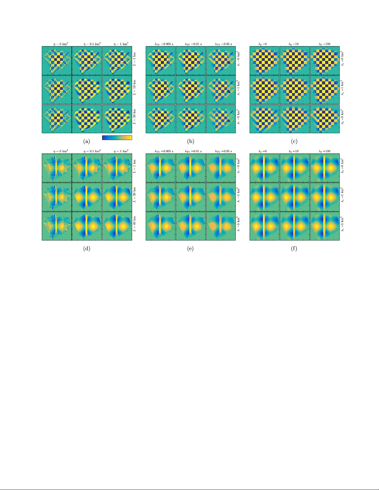
Loading comments...
Leave a Comment