A Novel Learnable Dictionary Encoding Layer for End-to-End Language Identification

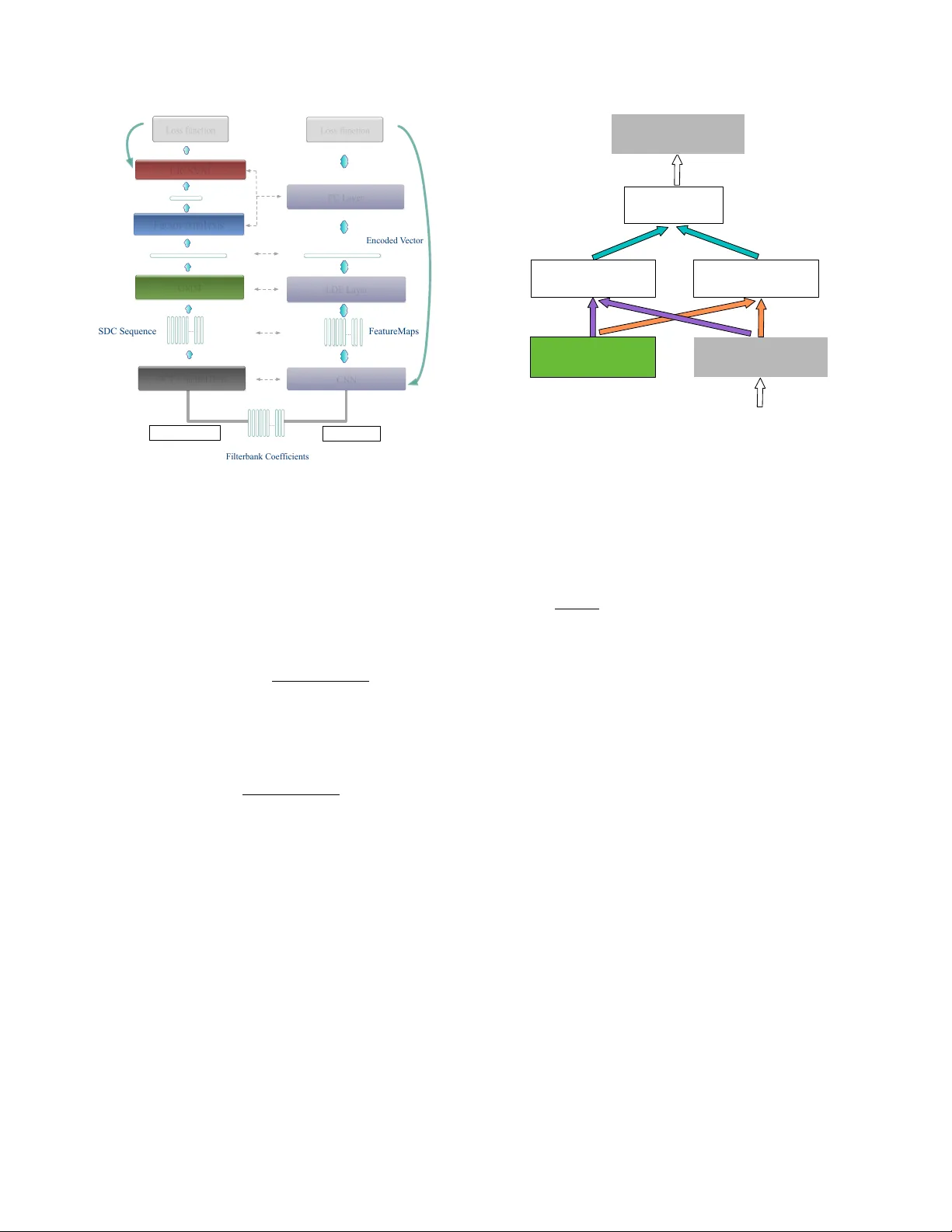
A NO VEL LEARNABLE DICTION AR Y ENCODING LA YER FOR END-TO-END LANGU A GE IDENTIFICA TION W eicheng Cai 1 , 3 , Zexin Cai 1 , Xiang Zhang 3 , Xiaoqi W ang 4 and Ming Li 1 , 2 ∗ 1 School of Electronics and Information T echnology , Sun Y at-sen Uni versity , Guangzhou, China 2 Data Science Research Center , Duke Kunshan Uni versity , Kunshan, China 3 T encent Inc., Beijing, China 4 Jiangsu Jinling Science and T echnology Group Limited ml442@duke.edu ABSTRA CT A nov el learnable dictionary encoding layer is proposed in this paper for end-to-end language identification. It is inline with the con ventional GMM i-v ector approach both theoretically and practi- cally . W e imitate the mechanism of traditional GMM training and Supervector encoding procedure on the top of CNN. The proposed layer can accumulate high-order statistics from v ariable-length in- put sequence and generate an utterance le vel fix ed-dimensional vec- tor representation. Unlike the con ventional methods, our ne w ap- proach pro vides an end-to-end learning framew ork, where the inher - ent dictionary are learned directly from the loss function. The dictio- naries and the encoding representation for the classifier are learned jointly . The representation is orderless and therefore appropriate for language identification. W e conducted a preliminary experiment on NIST LRE07 closed-set task, and the results reveal that our proposed dictionary encoding layer achieves significant error reduction com- paring with the simple av erage pooling. Index T erms — language identification (LID), end-to-end, dic- tionary encoding layer , GMM Supervector , variable length 1. INTR ODUCTION Language identification (LID) can be defined as a utterance lev el paralinguistic speech attribute classification task, in compared with automatic speech recognition, which is a “sequence-to-sequence” tagging task. There is no constraint on the lexicon words thus the training utterances and testing segments may ha ve completely dif- ferent content [1]. The goal, therefore, might be to find a robust and duration-inv ariant utterance le vel vector representation describ- ing the distributions of local features. In recent decades, in order to get the utterance level vector rep- resentation, dictionary learning procedure is widely used. A dictio- nary , which contains sev eral temporal orderless center components ( or units, words), can encode the v ariable-length input sequence into a single utterance le vel vector representation. V ector quantization (VQ) model, is one of the simplest text-independent dictionary mod- els [1]. It was introduced to speaker recognition in the 1980s [2]. The av erage quantization distortion is aggre gated from the frame-le vel ∗ This research was funded in part by the National Natural Science Foundation of China (61401524,61773413), Natural Science Foundation of Guangzhou City (201707010363), Science and T echnology Development Foundation of Guangdong Province (2017B090901045), National Ke y Re- search and Dev elopment Program (2016YFC0103905). residual towards to the K-means clustered codebook. The Gaus- sian Mixture Model (GMM) can be considered as an extension of the VQ model, in which the posterior assignments are soft [3, 4]. Once we ha ve a trained GMM, we can simply av erage the frame- lev el likelihood to generate the encoded utterance level likelihood score. Besides, we can move forward to accumulate the 0 th and 1 st order Baum-W elch statistics, and encode them into a high dimen- sional GMM Supervector [5]. VQ codebook and GMM are unsu- pervised and there is no exact physical meaning on its components. Another way to learn the dictionary is through phonetically-aware supervised training [6, 7]. In this method, a deep neural network (DNN) based acoustic model is trained. Each component in the dic- tionary represents a phoneme (or senone) physically , and the statis- tics is accumulated through senone posteriors, as is done in recently popular DNN i-vector approach [8, 9, 10]. A phonotactic tokenizer can be considered as a dictionary doing hard assignments with top-1 score [1]. Once we have a trained tokenizer , usually a bag-of-words (BoW) or N-gram model is used to form the encoded representation [11, 12]. These e xisting approaches hav e the advantage of accepting variable-length input and the encoded representation is in utterance lev el. Howe ver , when we mov e forward to modern the end-to-end learning pipeline, e.g. the neural network, especially for the fully- connected (FC) network, it usually requires a fixed-length input. In order to feed into the netw ork, as is done in [13, 14, 15, 16], the orig- inal input feature sequence has to be resized or cropped into multiple small fix ed-size se gments in frame le vel. This might be theoretically and practically not ideal for recognizing language, speaker or other paralinguistic information due to the need of a time-in variant rep- resentation from the entire arbitrary and potentially long duration length. T o deal with this issue, recently , in both [17, 18], similar tem- poral average pooling(T AP) layer is adopted in their neural network architectures. W ith the merit of T AP layer, the neural network have the ability to train input segments with random duration. In testing stage, the whole speech segments with arbitrary duration can be fed into the neural network. Compared with the simple T AP , the con ventional dictionary learning have the ability to learn a finer global histogram to demon- strate the feature distribution better, and it can accumulate high order statistics. In computer vision community , especially in image scene classification, texture recognition, action recognition tasks, modern con volutional neural network (CNN) usually bound to the conv en- tional dictionary learning methods together to get a better encoding representation. For example, NetVLAD [19], NetFV [20], Bilinear Pooling [21], and Deep TEN [22] are proposed and achieved great success. This motiv ates us to implement the conv entional GMM and Su- pervector mechanism into our end-to-end LID neural network. As the major contribution of this paper , we introduce a novel learn- able dictionary encoding (LDE) layer, which combines the entire dictionary learning and vector encoding pipeline into a single layer for end-to-end deep CNN. The LDE layer imitates the mechanism of conv entional GMM and GMM Supervector , but learned directly from the loss function. This representation is orderless which might be suitable for LID and many other test-independent paralinguistic speech attribute recognition tasks. The LDE layer acts as a smart pooling layer integrated on top of con volutional layers, accepting variable length inputs and providing output as an utterance level vector representation. By allowing variable-length inputs, the LDE layer makes the deep learning framework more flexible to train ut- terances with arbitrary duration. In these sense, it is inline with the classical GMM i-vector [23] method both theoretically and practi- cally . 2. METHODS 2.1. GMM Superv ector In con ventional GMM Supervector approach , all frames of features in training dataset are grouped together to estimate a uni versal back- ground model (UBM). Giv en a C component GMM UBM model λ with λ c = { p c , µ c , Σ c } , c = 1 , · · · , C and an utterance with a L frame feat ure sequence { x 1 , x 2 , · · · , x L } , the 0 th and c entered 1 st order Baum-W elch statistics on the UBM are calculated as follows: N c = L X t =1 P ( c | x t , λ ) (1) F c = L X t =1 P ( c | x t , λ ) · r tc (2) where c = 1 , · · · , C is the GMM component index and P ( c | x t , λ ) is the occupanc y probability for x t on λ c . r tc = x t − µ c denotes as a residual between t th frame feature and the mean of the GMM’ s c th component. The corresponding centered mean supervector ˜ F is generated by concatenating all the ˜ F c together: ˜ F c = P L t =1 P ( c | x t , λ ) · r tc P L t =1 P ( c | x t , λ ) . (3) 2.2. LDE layer Motiv ated by GMM Supervector encoding procedure, the proposed LDE layer has the similar input-output structure. As demonstrated in Fig. 1, given an input temporal ordered feature sequence with the shape D × L (where D denotes the feature coefficients dimension, and L denotes the temporal duration length), LDE layer aggregates them over time. More specifically , it transforms them into an utter- ance le vel temporal orderless D × C vector representation, which is independent of length L . Different from conv entional approaches, we combine the dic- tionary learning and vector encoding into a single LDE layer on top of the front-end CNN, as shown in Fig. 2. The LDE layer si- multaneously learns the encoding parameters along with an inherent … LDE Layer ( #Components = C ) … D C ⇥ D L ⇥ Fig. 1 . The input-out structure of LDE layer. It recei ves input feature sequence with variable length, produces an encoded utterance level vector with fix ed dimension dictionary in a fully supervised manner . The inherent dictionary is learned from the distribution of the descriptors by passing the gra- dient through assignment weights. During the training process, the updating of extracted con volutional features can also benefit from the encoding representations. The LDE layer is a directed acyclic graph and all the compo- nents are dif ferentiable w .r .t the input X and the learnable parame- ters. Therefore, the LDE layer can be trained end-to-end by standard stochastic gradient descent with backpropagation. Fig. 3 illustrates the forward diagram of LDE layer . Here, we introduce tw o groups of learnable parameters. One is the dictionary component center , noted as µ = { µ 1 , · · · µ c } . The other one is assigned weights, which is designed to imitate the P ( c | x t , λ ) , noted as w . Consider assigning weights from the features to the dictio- nary components. Hard-assignment provides a binary weight for each feature x t , which corresponds to the nearest dictionary components. The c th element of the assigning vector is given by w tc = δ ( k r tc k 2 = min {k r t 1 k , · · · k r tC k} ) , where δ is the indi- cator function (outputs 0 or 1). Hard-assignment does not consider the dictionary component ambiguity and also makes the model non- differentiable. Soft-weight assignment addresses this issue by as- signing the feature to each dictionary component. The non-neg ativ e assigning weight is giv en by a softmax function, w tc = exp( − β k r tc k 2 ) P C m =1 exp( − β k r tm k 2 ) (4) where β is the smoothing factor for the assignment. Soft- assignment assumes that different clusters hav e equal scales. In- spired by GMM, we further allow the smoothing factor s c for each dictionary center u c to be learnable: w tc = exp( − s c k r tc k 2 ) P C m =1 exp( − s i k r tm k 2 ) (5) which provides a finer modeling of the feature distrib utions. Giv en a set of L frames feature sequence { x 1 , x 2 , · · · , x L } and a learned dictionary center µ = { µ 1 , · · · µ c } , each frame of FC Layer LR/SVM Loss function Loss function GMM LDE Layer Factor Analysis GMM i-vector End-to-End backward backward F i l t e rba nk Coe f fi c i e nt s S D C S e que nc e F e a t ure M a ps Supervector i-vector E nc ode d V e c t or … … … DCT + Shifted Delta CNN Fig. 2 . Comparison of GMM i-v ector approach and end-to-end neu- ral network with LDE layer feature x t can be assigned with a weight w tc to each component µ c and the corresponding residual v ector is denoted by r tc = x t − u c , where t = 1 , · · · L and c = 1 , · · · C . Gi ven the assignments and the residual vector , similar to conv entional GMM Supervector , the residual encoding model applies an aggregation operation for every dictionary component center µ c : e c = L X t =1 e tc = P L t =1 ( w tc · r tc ) P L t =1 w tc (6) It’ s complicated to compute the the explicit expression for the gradients of the loss ` with respect to the layer input x t . In order to facilitate the deri vation we simplified it as e c = P L t =1 ( w tc · r tc ) L (7) The LDE layer concatenates the aggreg ated residual vectors with assigned weights. The resulted encoder outputs a fixed dimen- sional representation E = { e 1 , · · · e C } (independent of the se- quence length L). As is typical in con ventional GMM Supervector/i- vector , the resulting vectors are normalized using the length normal- ization [24]. W e implement the LDE layer similar as described in [22], and more detail about the explicit e xpression for the gradients of the loss ` with respect to the layer input and the parameters can refer to [22]. 2.3. Relation to traditional dictionary learning and T AP layer Dictionary learning is usually learned from the distribution of the de- scriptors in an unsupervised manner . K-means learns the dictionary using hard-assignment grouping. GMM is a probabilistic version of K-means, which allows a finer modeling of the feature distribu- tions. Each cluster is modeled by a Gaussian component with its own mean, v ariance and mixture weight. The LDE layer makes the inherent dictionary differentiable w .r .t the loss function and learns V ariable Length Input Dictionary Components Residuals Aggregate Assign W eights Encoded V ector Fig. 3 . The forward diagram within the LDE layer the dictionary in a supervised manner. T o see the relationship of the LDE to K- means, consider Fig. 3 with omission of the residual v ec- tors and let smoothing f actor β → ∞ . W ith these modifications, the LDE layer acts like K-means. The LDE layer can also be re- garded as a simplified v ersion of GMM, that allows different scaling (smoothing) of the clusters. Letting C = 1 and fixing µ = 0, the LDE layer simplifies to T AP layer ( e = P L t =1 x t L ) . 3. EXPERIMENTS 3.1. Data description W e conducted experiments on 2007 NIST Language Recognition Evaluation(LRE). Our training corpus including Callfriend datasets, LRE 2003, LRE 2005, SRE 2008 datasets, and dev elopment data for LRE07. The total training data is about 37000 utterances. The task of interest is the closed-set language detection. There are totally 14 target languages in testing corpus, which included 7530 utterances split among three nomial durations: 30, 10 and 3 seconds. 3.2. GMM i-vector system For better result comparison, we b uilt a referenced GMM i-vector system based on Kaldi toolkit [25]. Raw audio is conv erted to 7-1- 3-7 based 56 dimensional shifted delta coefficients (SDC) feature, and a frame-level energy-based voice activity detection (V AD) se- lects features corresponding to speech frames. All the utterances are split into short segments no more than 120 seconds long. A 2048 components full covariance GMM UBM is trained, along with a 600 dimensional i-vector extractor , follo wed by length normalization and multi-class logistic regression. 3.3. End-to-end system Audio is con verted to 64-dimensional log mel-filterbank coef ficients with a frame-length of 25 ms, mean-normalized ov er a sliding win- dow of up to 3 seconds. The same V AD processing as in GMM T able 1 . Performance on the 2007 NIST LRE closed-set task System System Description Feature Encoding Method C avg (%) E E R (%) ID 3s 10s 30s 3s 10s 30s 1 GMM i-vector SDC GMM Supervector 20.46 8.29 3.02 17.71 7.00 2.27 2 CNN-T AP CNN FeatureMaps T AP 9.98 3.24 1.73 11.28 5.76 3.96 3 CNN-LDE(C=16) CNN FeatureMaps LDE 9.61 3.71 1.74 8.89 2.73 1.13 4 CNN-LDE(C=32) CNN FeatureMaps LDE 8.70 2.94 1.41 8.12 2.45 0.98 5 CNN-LDE(C=64) CNN FeatureMaps LDE 8.25 2.61 1.13 7.75 2.31 0.96 6 CNN-LDE(C=128) CNN FeatureMaps LDE 8.56 2.99 1.63 8.20 2.49 1.12 7 CNN-LDE(C=256) CNN FeatureMaps LDE 8.77 3.01 1.97 8.59 2.87 1.38 8 Fusion ID2 + ID5 - - 6.98 2.33 0.91 6.09 2.26 0.87 T able 2 . Our front-end CNN configuration layer output size downsample channels blocks con v1 64 × L in False 16 - res1 64 × L in False 16 3 res2 32 × L in 2 T rue 32 4 res3 16 × L in 4 T rue 64 6 res4 8 × L in 8 T rue 128 3 avgpool 1 × L in 8 - 128 - reshape 128 × L out , L out = L in 8 - - - i-vector baseline system is used here. For improving the data load- ing ef ficiency , all the utterances are split into short segments no more than 60s long , according to the V AD flags. The receptiv e field size of a unit can be increased by stacking more layers to make the network deeper or by sub-sampling. Modern deep CNN architectures like Residual Networks [26] use a combina- tion of these techniques. Therefore, in order to get higher abstract representation better for utterances with long duration, we design a deep CNN based on the well-known ResNet-34 layer architecture, as is described in T able 2. For CNN-T AP system, a simple average pooling layer followed with FC layer is b uilt on top of the font-end CNN. For CNN-LDE system, the av erage pooling layer is replaced with a LDE layer . The network is trained using a cross entropy loss. The model is trained with a mini-batch, whose size v aries from 96 to 512 consider- ing dif ferent model parameters. The network is trained for 90 epochs using stochastic gradient descent with momentum 0.9 and weight de- cay 1e-4. W e start with a learning rate of 0.1 and di vide it by 10 and 100 at 60th and 80th epoch. Because we have no separated v alida- tion set, even though there might exist some model checkpoints can achiev e better performance, we only use the model after the last step optimization. For each training step, an integer L within [200 , 1000] interval is randomly generated, and each data in the mini-batch is cropped or extended to L frames. The training loss tendency of our end-to-end CNN-LDE neural network is demonstrated in Fig. 4. It shows that our neural network with LDE layer is traninable and the loss can con verge to a small v alue. In testing stage, all the 3s, 10s, and 30s duration data is tested on the same model. Because the duration length is arbitrary , we feed the testing speech utterance to the trained neural network one by one. In order to get the system fusion results of ID8 in T able 1, we randomly crop several additional training data corresponding to the separated 30s, 10s, 3s duration tasks. The score level system fusion weights are all trained on them. Fig. 4 . Loss duraing CNN-LDE training stage, smoothed with each 400 steps 3.4. Evaluation T able 1 shows the performance on the 2007 NIST LRE closed-set task. The performance is reported in average detection cost C avg and equal error rate (EER). Both CNN-T AP and CNN-LDE system achiev e significant performance improvement comparing with con- ventional GMM i-v ector system. For our purpose in exploring encoding method for end-to-end neural network, we focus the comparison on system ID2 and ID3- ID7. The CNN-LDE system outperforms the CNN-T AP system with all different number of dictionary components. When the numbers of dictionary component increased from 16 to 64, the performance improv ed insistently . Howev er , once dictionary component numbers are lar ger than 64, the performance decreased perhaps because of ov erfitting. Comparing with CNN-T AP , the best CNN-LDE-64 system achiev es significant performance improvement especially with re- gard to EER. Besides, their score le vel fusion result further improves the system performance significantly . 4. CONCLUSIONS In this paper, we imitate the GMM Supervector encoding procedure and introduce a LDE layer for end-to-end LID neural network. The LDE layer acts as a smart pooling layer integrated on top of con volu- tional layers, accepting arbitrary input lengths and providing output as a fixed-length representation. Unlike the simple T AP , it rely on a learnable dictionary and can accumulate more discriminativ e statis- tics. The experiment results show the superior and complementary of LDE comparing with T AP . 5. REFERENCES [1] T . Kinnunen and H. Li, “ An overvie w of text-independent speaker recognition: From features to supervectors, ” Speech Communication , vol. 52, no. 1, pp. 12–40, 2010. [2] F . Soong, A. E. Rosenberg, J. BlingHwang, and L. R. Rabiner , “Report: A vector quantization approach to speaker recogni- tion, ” At & T T echnical Journal , vol. 66, no. 2, pp. 387–390, 1985. [3] D.A. Reynolds and R.C. Rose, “Robust text-independent speaker identification using gaussian mixture speaker models, ” IEEE T ransactions on Speech & Audio Pr ocessing , vol. 3, no. 1, pp. 72–83, 1995. [4] D.A. Reynolds, T .F . Quatieri, and R.B. Dunn, “Speaker ver - ification using adapted gaussian mixture models, ” in Digital Signal Pr ocessing , 2000, p. 1941. [5] W .M. Campbell, D.E. Sturim, and D A Reynolds, “Support vec- tor machines using gmm supervectors for speaker verification, ” IEEE Signal Pr ocessing Letters , v ol. 13, no. 5, pp. 308–311, 2006. [6] Y . Lei, N. Scheffer , L. Ferrer, and M. McLaren, “ A novel scheme for speaker recognition using a phonetically-aw are deep neural network, ” in ICASSP 2014 . [7] M. Li and W . Liu, “Speaker verification and spoken language identification using a generalized i-vector framew ork with pho- netic tokenizations and tandem features, ” in INTERSPEECH 2014 . [8] M. Mclaren, Y . Lei, and L. Ferrer, “ Advances in deep neural network approaches to speaker recognition, ” in IEEE Interna- tional Confer ence on Acoustics, Speech and Signal Pr ocessing , 2015, pp. 4814–4818. [9] F . Richardson, D. Reynolds, and N. Dehak, “Deep neural net- work approaches to speaker and language recognition, ” IEEE Signal Pr ocessing Letters , v ol. 22, no. 10, pp. 1671–1675, 2015. [10] D. Snyder , D. Garcia-Romero, and D. Po vey , “Time delay deep neural network-based universal background models for speaker recognition, ” in ASRU 2016 , pp. 92–97. [11] G. Gelly , J. L. Gauv ain, V . B. Le, and A. Messaoudi, “ A divide- and-conquer approach for language identification based on re- current neural networks, ” in INTERSPEECH 2016 , pp. 3231– 3235. [12] M. Li, L. Liu, W . Cai, and W . Liu, “Generalized i-vector repre- sentation with phonetic tokenizations and tandem features for both te xt independent and text dependent speaker verification, ” Journal of Signal Pr ocessing Systems , vol. 82, no. 2, pp. 207– 215, 2016. [13] I. Lopez-Moreno, J. Gonzalez-Dominguez, O. Plchot, D. Mar- tinez, J. Gonzalez-Rodriguez, and P . Moreno, “ Automatic lan- guage identification using deep neural networks, ” in ICASSP 2014 . [14] J. Gonzalez-Dominguez, I. Lopez-Moreno, H. Sak, J. Gonzalez-Rodriguez, and P . J Moreno, “ Automatic language identification using long short-term memory re- current neural networks, ” in Pr oc. INTERSPEECH 2014 , 2014. [15] R. Li, S. Mallidi, L. Bur get, O. Plchot, and N. Dehak, “Ex- ploiting hidden-layer responses of deep neural networks for language recognition, ” in INTERSPEECH , 2016. [16] M. Tkachenko, A. Y amshinin, N. L yubimov , M. Koto v , and M. Nastasenko, “Language identification using time delay neu- ral network d-vector on short utterances, ” 2016. [17] L. Chao, M. Xiaokong, J. Bing, L. Xiangang, Z. Xuewei, L. Xiao, C. Y ing, K. Ajay , and Z. Zhenyao, “Deep speaker: an end-to-end neural speaker embedding system, ” 2017. [18] D. Snyder , P . Ghahremani, D. Povey , D. Garcia-Romero, Y . Carmiel, and S. Khudanpur, “Deep neural network-based speaker embeddings for end-to-end speak er v erification, ” in SLT 2017 , pp. 165–170. [19] R. Arandjelovic, P . Gronat, A. T orii, T . Pajdla, and J. Si vic, “Netvlad: Cnn architecture for weakly supervised place recog- nition, ” in CVPR 2016 , 2016, pp. 5297–5307. [20] S. Simonyan, A. V edaldi, and A. Zisserman, “Deep fisher net- works for large-scale image classification, ” in NIPS 2013 , pp. 163–171. [21] T . Lin, A. Roychowdhury , and S. Maji, “Bilinear cnns for fine- grained visual recognition, ” in IEEE International Confer ence on Computer V ision , 2016, pp. 1449–1457. [22] H. Zhang, J. Xue, and K. Dana, “Deep ten: T exture encoding network, ” in CVPR 2017 . [23] N. Dehak, P . K enny , R. Dehak, P . Dumouchel, and P . Ouel- let, “Front-end factor analysis for speaker verification, ” IEEE T ransactions on Audio, Speech, and Language Processing , vol. 19, no. 4, pp. 788–798, 2011. [24] Daniel Garcia-Romero and Carol Y Esp y-W ilson, “ Analysis of i-vector length normalization in speaker recognition systems., ” in INTERSPEECH 2011 , pp. 249–252. [25] D. Pov ey and A. et al. Ghoshal, “The kaldi speech recognition toolkit, ” in ASRU 2011 . [26] K. He, X. Zhang, S. Ren, and J. Sun, “Deep residual learning for image recognition, ” in CVPR 2016 , 2016, pp. 770–778.