Insights into End-to-End Learning Scheme for Language Identification

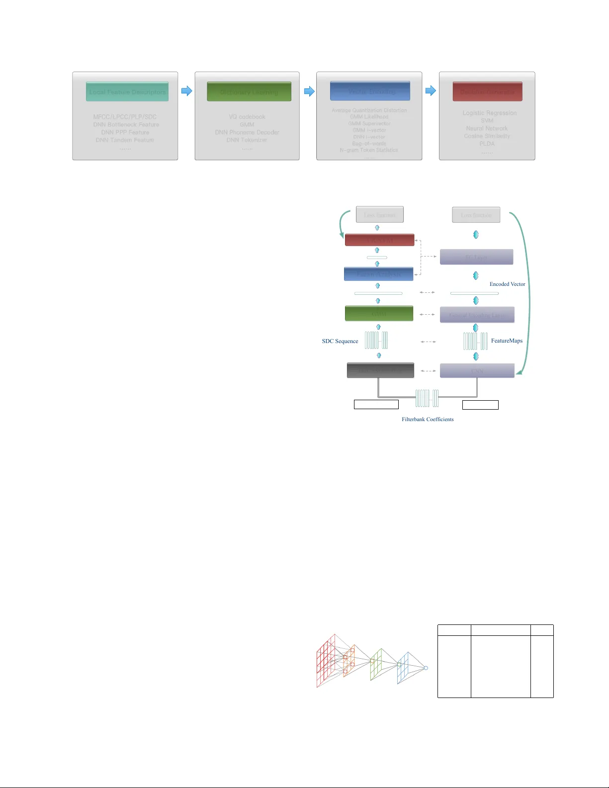
INSIGHTS INTO END-T O-END LEARNING SCHEME FOR LANGU A GE IDENTIFICA TION W eicheng Cai 1 , Zexin Cai 1 W enbo Liu 3 , Xiaoqi W ang 4 , and Ming Li 1 , 2 ∗ 1 School of Electronics and Information T echnology , Sun Y at-sen Univ ersity , Guangzhou, China 2 Data Science Research Center , Duke Kunshan Uni versity , Kunshan, China 3 Department of Electrical and Computer Engineering, Carnegie Mellon Uni versity , Pittsbur gh, USA 4 Jiangsu Jinling Science and T echnology Group Limited ml442@duke.edu ABSTRA CT A no vel interpretable end-to-end learning scheme for language identification is proposed. It is in line with the classical GMM i- vector methods both theoretically and practically . In the end-to-end pipeline, a general encoding layer is employed on top of the front- end CNN, so that it can encode the variable-length input sequence into an utterance level vector automatically . After comparing with the state-of-the-art GMM i-vector methods, we give insights into CNN, and rev eal its role and effect in the whole pipeline. W e further introduce a general encoding layer, illustrating the reason why they might be appropriate for language identification. W e elaborate on sev eral typical encoding layers, including a temporal av erage pool- ing layer , a recurrent encoding layer and a nov el learnable dictionary encoding layer . W e conducted experiment on NIST LRE07 closed- set task, and the results show that our proposed end-to-end systems achiev e state-of-the-art performance. Index T erms — language identification (LID), end-to-end, en- coding layer , utterance lev el, variable length 1. INTR ODUCTION Language identification (LID) can be defined as a utterance level par- alinguistic speech attribute classification task, in compared with au- tomatic speech recognition, which is a “sequence-to-sequence” tag- ging task. There is no constraint on the le xicon words thus the train- ing utterances and testing segments may have completely different contents [1]. The goal, therefore, might to find a robust and time- in variant utterance lev el vector representation describing the distri- bution of local features. In recent decades, we have witnessed that the classical Gaussian Mixture Model (GMM) i-v ector approach dominates many kinds of paralinguistic speech attribute recognition fields for its superior per - formance, simplicity and efficienc y [2, 3]. As shown in Fig. 1, the processing pipeline contains four main steps as follows: • Local feature descriptors, which manifest as a variable- length feature sequence, include hand-crafted acoustic level features, such as log mel-filterbank energies (Fbank), mel- frequency cepstral coef ficients (MFCC), perceptual linear prediction (PLP), shifted delta coefficients (SDC) features ∗ This research was funded in part by the National Natural Science Foundation of China (61401524,61773413), Natural Science Foundation of Guangzhou City (201707010363), Science and T echnology Development Foundation of Guangdong Province (2017B090901045), National Ke y Re- search and Dev elopment Program (2016YFC0103905). [1, 4], or automatically learned phoneme discriminant fea- tures from deep neural networks (DNN), such as bottleneck features [5, 6], phoneme posterior probability (PPP) features [7], and tandem features [8]. • Dictionary , which contains se veral orderless center compo- nents( or units, words), including vector quantization (VQ) codebooks learned by K-means [9], a universal background model (UBM) learned by GMM [10, 11] or a supervised phonetically-aware acoustic model learned by DNN [12, 13]. • V ector encoding. This procedure aggregates the variable- length feature sequence into an utterance level vector repre- sentation, based on the learned dictionary mentioned above. The typical examples are the well-known GMM Supervec- tor [14], the classical GMM i-vector [2] or recently popular DNN i-vector [15]. • Decision generator, includes logistic regression (LR), sup- port vector machine (SVM), and neural network for closed- set identification, cosine similarity or probabilistic linear dis- criminant analysis (PLD A) [16, 17] for open-set verification. Despite the great success, the baseline GMM i-vector methods remain room to be improved: First, the front-end process t o get i- vectors is totally unsupervised. Thus, the i-vectors we hav e extracted may ignore some patterns that might be useful for the back-end clas- sification. Second, the process to obtain i-vectors is comprised of a series hand-crafted or ad-hoc algorithmic components. Once fea- ture is extracted or front-end model is trained, they are fixed that can’t benefit from subsequent steps. For example, we often let the extracted i-vectors fixed and tune the back-end algorithm for better performance. Howe ver , no matter how superior the back-end algo- rithm is, we may still suffer from a local minima determined by the discrimination carried on i-vector . Therefore, the recent progress tow ards end-to-end learning opens up a new area for exploration [18, 19, 20, 21, 22, 23, 24]. The work in [24] introduced deep conv olutional neural Network (CNN) from image recognition, and proved its success on their own priv ate speaker recognition database. In both [20, 24], similar temporal av erage pooling (T AP) layer is adopted within their neural network architectures. T o the best of our knowledge, many of existing end-to-end works perform excellent on trial-and-error experiments, howe ver , there is no very clear explanation about why they perform so well, or how they might be further improved. In this paper, we explore both issues. As the first contribution, we giv e insights into a general learning scheme for end-to-end LID, with an emphasis on CNN and a encoding layer . W e explore how CNN can transform the variable- length input feature sequence into high-level representation, acting                             Fig. 1 . Four main steps in the con ventional processing pipeline as an automatic front-end feature extractor . Although the contextual information in conv olutional receptiv e field is captured, the fea- ture extracted by CNN is still with temporal order . The remaining question is: how to aggregate them together over the entire and po- tentially long duration length? Concerning about that, as our second contribution, we introduce a general encoding layer . W e provide its general structure and elaborate on several typical vector encoding layers, including a simple T AP layer , a recurrent encoding layer , and a learnable dictionary encoding (LDE) layer as well. 2. INSIGHTS 2.1. End-to-end learning scheme A comparison of con ventional approaches and the proposed end-to- end learning scheme is described in Fig. 2. In traditional methods like GMM i-v ector , each component is optimized in separate steps as illustrated with dif ferent colors. In our end-to-end learning scheme, the entire pipeline is learned in an integrated manner because the features, encoding layer and the encoded vector representation for the classifier are all learned jointly . There are two characteristics of our learning scheme sho wing the theoretical and practical compatibility with the classical GMM i-vector approach: First, each component of our neural network has its parallel equiv alent block tow ards to the classical GMM i-vector processing stream, as demonstrated in Fig. 2. Second, our neu- ral netw ork architectures accept v ariable-length speech inputs and learn an utterance level representation, which explores the strength of GMM i-vector based methods practically . 2.2. The role and effect of CNN CNN is a kind of specialized neural network for processing data with a kno wn grid-lik e topology and it uses learned filters to con volve the feature maps from the previous layer . One of the basic concepts in deep CNN is the receptiv e field, as dro wn in the left part of Fig. 3. A unit in CNN only depends on a region of the input and this region of the input is the receptiv e field for that unit [25]. The concept of receptiv e field is important for understanding how CNN can extract local feature descriptors automatically . Since anywhere outside the receptiv e field of a unit does not af fect the value of that unit, it is necessary to carefully control the recepti ve field, to ensure that it covers the entire rele vant input region. A sim- ple toy CNN is described in right part of Fig. 3. The input feature coefficient has 64 dimension, with L frames. After fi ve times conv o- lution, the recepti ve field of output units reach to 63, which not only cov er the entire feature coef ficients axis, b ut also a wide temporal context range. T o some extent, therefore, the con volution layer of CNNs oper- ates in an sliding windo w manner acting as a automatic local feature FC Layer LR/SVM Loss function Loss function GMM General Encoding Layer Factor Analysis GMM i-vector End-to-End backward backward F i l t e rba nk Coe f fi c i e nt s S D C S e que nc e F e a t ure M a ps Supervector i-vector E nc ode d V e c t or … … … DCT + Shifted Delta CNN Fig. 2 . Comparison of classical GMM i-vector approach and the proposed end-to-end learning scheme extractor . It learns temporal ordered feature representation automat- ically under the backward from loss function. Any feature sequence with variable-length can fed into CNN theoretically , and in our experiments, Fbank is adopted as the input. 2.3. General encoding layer Deep learning is well known for end-to-end modeling of hierarchical features, so what is the challenge of recognizing language pattern in an end-to-end way and why we need such proposed general encoding layer? The output featuremaps of CNN preserv e a relati ve temporal ar - layer shape RF input (64, L) 1 con v1 K=(3,3), S=2 3 con v2 K=(3,3), S=2 7 con v3 K=(3,3), S=2 15 con v4 K=(3,3), S=2 31 con v5 K=(3,3), S=2 63 Fig. 3 . Example diagram of con volutional recepti ve field General Encoding Layer … D in ⇥ L D out ⇥ C Fig. 4 . General encoding layer . It receives input feature sequence with variable length, produces an encoded utterance lev el vector with fixed dimension rangement of the giv en input feature sequence. A simple way is to concatenate the resulted globally ordered features together and fed it into the fully-connected (FC) layer for classification. Howe ver , this is theoretically and practically not ideal for rec- ognizing language, speak er or other paralinguistic information since we need a time-inv ariant representation instead of concatenation. Therefore, a general encoding layer , which can transfer the temporal ordered frame le vel local features with v ariable length into an tem- poral orderless utterance level vector representation is desirable for our end-to-end learning scheme. The general structure of encoding layer is demonstrated in Fig. 5. For a giv en input temporal ordered feature sequence with the shape D in × L (where D in denotes the feature dimension of local feature after CNN, and L denotes the temporal duration length after CNN), the encoding layer aggregates them over time. More specif- ically , it transforms them into a utterance lev el temporal orderless D out × C vector representation, which is independent of duration length L . W e introduce a ne w axis with shape C , because we can imitate the mechanism of conv entional K-means/GMM/DNN based dictio- nary model and design a dictionary to encode vector accumulating high order statistics. 3. ARCHITECTURES 3.1. CNN The receptive field size of a unit can be increased by stacking more layers to make the network deeper or by sub-sampling. Modern deep CNN architectures like Residual Networks [26] use a combination of these techniques. Therefore, in order to get higher abstract repre- sentation better for utterances with long duration, we design a CNN based on the well-kno wn deep ResNet architecture. The detailed network structure is the same as described in [27]. 3.2. T AP lay er The simplest encoding layer might equally pool the CNN extracted features over time. This encoding procedure is context-independent because it just accumulate the mean statistics and doesn’t rely on the temporal structure of feature. 3.3. Recurrent encoding layer The other way to encode vector is to employ recurrent layer , such as long short term Memory (LSTM) layer [28], gated recurrent unit (GR U) layer [29]. It operates on top of the extracted frame-le vel features to capture the temporal structure of speech segments into a single representation. This encoding procedure is context-dependent because it rely on the temporal order of feature sequence. Because recurrent layer can make full use of the context of fea- ture sequences in forward directions, we regard the last output vector of this recurrent layer as the encoded representation and put it only into the following fully-connected layer , as is in Fig. 5. 3.4. LDE layer The simple av erage pooling might not be the best way to demon- strate the feature distribution and conv entional methods always rely on an dictionary learning procedure like K-means/GMM/DNN, to accumulate more discriminativ e statistics. Inspired by this, we introduce a nov el LDE Layer to accumulate statistics on more detailed units. It combines the entire dictionary learning and vector encoding pipeline into a single layer for end- to-end learning. The LDE Layer imitates the mechanism of GMM Supervector , b ut learned directly from the loss function. This repre- sentation is orderless which is suitable for te xt-independent applica- tions, such as LID. The LDE Layer acts as a pooling layer inte grated on top of conv olutional layers, accepting arbitrary input sizes and providing output as a fix ed dimensional representation. More details can refer to [27]. 4. EXPERIMENTS 4.1. Data description For better results reproduction, we conducted experiments on 2007 NIST Language Recognition Evaluation(LRE), because the initial data processing and the referenced GMM/DNN i-vector baseline systems hav e their ready-made recipe developed in the Kaldi toolkit [30]. Our training corpus including Callfriend datasets, LRE 2003, LRE 2005, SRE 2008 datasets and development data for LRE07. The total training data is about 37000 utterances. The task of inter- est is the closed-set language detection. There are totally 14 target languages in testing corpus, which included 7530 utterances split among three nomial durations: 30, 10 and 3 seconds. 4.2. Con ventional systems As for the GMM i-vector system, raw audio is conv erted to 7-1- 3-7 based 56 dimensional SDC feature, and a frame-level energy- based V AD selects features corresponding to speech frames. All the utterances are split into short segments no more than 120 seconds long. A 2048 components full cov ariance GMM UBM is trained, along with a 600 dimensional i-vector extractor , followed by length normalization and multi-class logistic regression. The DNN i-vector system uses an extra DNN phoneme decoder containing 5621 senones, which is trainied with Fisher English database. The sufficient statistics is accumulated through the DNN senone posteriors and the DNN-initialized UBM. T o av oid training additional DNN acoustic model, we use DNN PPP feature, rather than DNN bottleneck feature. The 5621 dimen- sional senone posteriors are conv erted into 52 dimensional PPP fea- ture by log transform, principal component analysis (PCA) reduction and a mean-normalization over a sliding windo w of up to 3 second. For DNN tandem system, the 56 dimensional SDC feature and the 52 dimensional PPP feature is concatenated at feature le vel to train GMM UBM model. LSTM/GRU (a) T AP layer (b) Recurrent encoding layer (c) LDE layer … … T AP Layer … … LDE Layer (#Compoents =C) … D ⇥ L D D in ⇥ L D out D ⇥ C D ⇥ L Fig. 5 . T ypical encoding layers. They all receiv e variable-length sequence, produce encoded utterance le vel vector with fix ed dimension 4.3. End-to-end system Audio is conv erted to 64-dimensional Fbank with a frame-length of 25 ms, mean-normalized ov er a sliding window of up to 3 seconds. The same voice activity detection (V AD) processing as in GMM i- vector baseline system is used here. The network is trained using a cross entropy loss. The network is trained for 90 epochs using stochastic gradient descent. W e start with a learning rate of 0.1 and divide it by 10 and 100 at 60th and 80th epoch. For recurrent GR U/LSTM layer , a two layer structure with its hidden and output dimension equal to the input vector dimension is adopted. The dictionary component amounts in LDE layer are 64. For each training step, an integer L within [200 , 1000] interval is randomly generated, and each data in the mini-batch is cropped or extended to L frames. In testing stage, all the 3s, 10s, and 30s duration data is tested on the same model. Because the duration length is arbitrary , we feed the testing speech utterance to the trained neural network one by one. 4.4. Evaluation T able 1 shows the performance on the 2007 NIST LRE closed-set task. The performance is reported in average detection cost C avg and equal error rate (EER). The con ventional system results start from ID1 to ID5, and the DNN PPP feature system achiev es the best result. For ID2 to ID5, additional speech data with transcription and an extra DNN phoneme decoder is required, while our end-to-end systems only rely on the acoustic le vel feature of LID data. Comparing with GMM i-vector , our end-to-end systems achieve C avg and EER reduction in a large gap. Even comparing with those DNN acoustic model based sys- tems, our final best CNN-LDE system achie ves comparable perfor- mance with DNN PPP feature system, outperforming the rest of con- ventional systems in T able 1 significantly . It’ s very interesting that although recurrent layer introduces much more parameters comparing with T AP , it results in a slightly degraded performance. Specially , when the full 30s duration utter- ance is fed into our CNN-GRU/CNN-LSTM neural network trained within 1000 frames (10s), it suffers from “the curse of sentence length” [31]. The performance drops sharply and almost equals to T able 1 . Performance on the 2007 NIST LRE closed-set task System System Description C avg (%) /E E R (%) ID 3s 10s 30s 1 GMM i-vector 20.46/17.71 8.29/7.00 3.02/2.27 2 DNN i-vector 14.64/12.04 6.20/3.74 2.601.29 3 DNN PPP Feature 8.00/6.90 2.20/1.43 0.61/0.32 4 DNN T andem Feature 9.85/7.96 3.161.95 0.97/0.51 5 DNN Phonotactic[22] 18.59/12.79 6.28/4.21 1.34/0.79 6 RNN D&C[22] 22.67/15.57 9.45/6.81 3.28/3.25 7 LSTM-Attention[21] -/14.72 -/- -/- 8 CNN-T AP 9.98/11.28 3.24/5.76 1.73/3.96 9 CNN-GRU 11.31/10.74 5.49/6.40 -/- 10 CNN-LSTM 10.17/9.80 4.66/4.26 -/- 11 CNN-LDE 8.25/7.75 2.61/2.31 1.13/0.96 random guess. In addition, many of previous works [19, 21] em- ploying RNN only report success results on short utterance ( ≤ 3s). Therefore, we can infer that although recurrent layer can deal with variable length inputs theoretically , it might be not suitable for the testing task with wide duration range and particularly with duration that are much longer than those used for training. The success of T AP and LDE layer inspires us that for this kind of paralinguistic speech attribute recognition tasks, it might be more necessary to get utterance level representation describing the conte xt-independent feature distribution rather than the temporal structure. 5. CONCLUSIONS In this paper we present a novel end-to-end learning scheme for LID. W e gi ve insights into its relationship with classical GMM i-vector in both theory and practice. W e analysis the role and effect of each components in the end-to-end pipeline in detail and discuss the rea- son why they might to be appropriate for LID. The results is very re- markable e ven though we only use the acoustic le vel information. In addition, as is done in con ventional i-vector based approach, we can extend the basic learning scheme with phoneme discriminant feature or phonetically-aware dictionary encoding methods in the future. 6. REFERENCES [1] T . Kinnunen and H. Li, “ An ov erview of text-independent speaker recognition: From features to supervectors, ” Speech Communication , vol. 52, no. 1, pp. 12–40, 2010. [2] N. Dehak, P . Kenn y , R. Dehak, P . Dumouchel, and P . Ouel- let, “Front-end factor analysis for speaker verification, ” IEEE T ransactions on Audio, Speech, and Language Pr ocessing , vol. 19, no. 4, pp. 788–798, 2011. [3] N. Dehak, P .A. T orres-Carrasquillo, D. Reynolds, and R. De- hak, “Language recognition via i-vectors and dimensionality reduction, ” in INTERSPEECH 2016 , pp. 857–860. [4] H. Li, B. Ma, and K. Lee, “Spoken language recognition: From fundamentals to practice, ” Proceedings of the IEEE , vol. 101, no. 5, pp. 1136–1159, 2013. [5] P . Matejka, L. Zhang, T . Ng, H. Mallidi, O. Glembek, J. Ma, and B. Zhang, “Neural network bottleneck features for lan- guage identification, ” Pr oc. IEEE Odyssey , pp. 299–304, 2014. [6] Y . Song, X. Hong, B. Jiang, R. Cui, I. Mcloughlin, and L. Dai, “Deep bottleneck network based i-vector representation for language identification, ” 2015. [7] M. Li, L. Liu, W . Cai, and W . Liu, “Generalized i-v ector repre- sentation with phonetic tokenizations and tandem features for both text independent and text dependent speaker v erification, ” Journal of Signal Pr ocessing Systems , vol. 82, no. 2, pp. 207– 215, 2016. [8] F . Richardson, D. Reynolds, and N. Dehak, “Deep neural net- work approaches to speaker and language recognition, ” IEEE Signal Processing Letters , vol. 22, no. 10, pp. 1671–1675, 2015. [9] F . Soong, A. E. Rosenber g, J. BlingHwang, and L. R. Rabiner , “Report: A vector quantization approach to speaker recogni- tion, ” At & T T echnical Journal , vol. 66, no. 2, pp. 387–390, 1985. [10] D.A. Re ynolds and R.C. Rose, “Rob ust text-independent speaker identification using gaussian mixture speaker models, ” IEEE T ransactions on Speech & Audio Pr ocessing , vol. 3, no. 1, pp. 72–83, 1995. [11] D.A. Reynolds, T .F . Quatieri, and R.B. Dunn, “Speaker ver - ification using adapted gaussian mixture models, ” in Digital Signal Pr ocessing , 2000, p. 1941. [12] Y . Lei, N. Schef fer, L. Ferrer, and M. McLaren, “ A novel scheme for speaker recognition using a phonetically-aware deep neural network, ” in ICASSP 2014 . [13] M. Li and W . Liu, “Speaker verification and spoken language identification using a generalized i-vector framew ork with pho- netic tokenizations and tandem features, ” in INTERSPEECH 2014 . [14] W .M. Campbell, D.E. Sturim, and DA Reynolds, “Support vector machines using gmm supervectors for speaker verifi- cation, ” IEEE Signal Processing Letters , vol. 13, no. 5, pp. 308–311, 2006. [15] D. Snyder , D. Garcia-Romero, and D. Povey , “Time delay deep neural network-based universal background models for speaker recognition, ” in ASRU 2016 , pp. 92–97. [16] S.J.D. Prince and J.H. Elder , “Probabilistic linear discriminant analysis for inferences about identity , ” in ICCV 2007 , pp. 1–8. [17] P . K enny , “Bayesian speaker v erification with heavy tailed pri- ors, ” OD YSSEY 2010 . [18] I. Lopez-Moreno, J. Gonzalez-Dominguez, O. Plchot, D. Mar- tinez, J. Gonzalez-Rodriguez, and P . Moreno, “ Automatic lan- guage identification using deep neural networks, ” in ICASSP 2014 . [19] J. Gonzalez-Dominguez, I. Lopez-Moreno, H. Sak, J. Gonzalez-Rodriguez, and P . J Moreno, “ Automatic language identification using long short-term memory re- current neural networks, ” in Proc. INTERSPEECH 2014 , 2014. [20] D. Snyder , P . Ghahremani, D. Povey , D. Garcia-Romero, Y . Carmiel, and S. Khudanpur, “Deep neural network-based speaker embeddings for end-to-end speaker verification, ” in SLT 2017 , pp. 165–170. [21] W . Geng, W . W ang, Y . Zhao, X. Cai, and B. Xu, “End-to-end language identification using attention-based recurrent neural networks, ” in INTERSPEECH , 2016, pp. 2944–2948. [22] G. Gelly , J. L. Gauvain, V . B. Le, and A. Messaoudi, “ A divide- and-conquer approach for language identification based on re- current neural networks, ” in INTERSPEECH 2016 , pp. 3231– 3235. [23] J. Ma, Y . Song, I. Mcloughlin, W . Guo, and L. Dai, “End-to- end language identification using high-order utterance repre- sentation with bilinear pooling, ” in INTERSPEECH 2017 , pp. 2571–2575. [24] L. Chao, M. Xiaok ong, J. Bing, L. Xiang ang, Z. Xuewei, L. Xiao, C. Y ing, K. Ajay , and Z. Zhenyao, “Deep speaker: an end-to-end neural speaker embedding system, ” 2017. [25] W . Luo, Y . Li, R. Urtasun, and R. Zemel, “Understanding the effecti ve receptiv e field in deep conv olutional neural net- works, ” 2017. [26] K. He, X. Zhang, S. Ren, and J. Sun, “Deep residual learning for image recognition, ” in CVPR 2016 , 2016, pp. 770–778. [27] W . Cai, Z. Cai, X. Zhang, and M. Li, “A novel learnable dic- tionary encoding layer for end-to-end language identification, ” in ICASSP 2018 . [28] A. Gra ves, Long Short-T erm Memory , Springer Berlin Heidel- berg, 2012. [29] J. Chung, C. Gulcehre, K. Cho, and Y . Bengio, “Empiri- cal evaluation of gated recurrent neural networks on sequence modeling, ” arXiv pr eprint arXiv:1412.3555 , 2014. [30] D. Po vey and A. et al. Ghoshal, “The kaldi speech recognition toolkit, ” in ASR U 2011 . [31] K. Cho, B. V . ¨ enboer , D. Bahdanau, and Y . Bengio, “On the properties of neural machine translation: Encoder-decoder ap- proaches, ” arXiv pr eprint arXiv:1409.1259 , 2014.