Random Switching for High Performance DC-DC Power Converters
Random Pulse Width Modulation (RPWM) has been successfully applied in power electronics for nearly 30 years. The effects of the various possible RPWM strategies on the Power Spectral Density have been thoroughly studied. Despite the effectiveness of …
Authors: Jacques Naude, Ivan Hofsajer
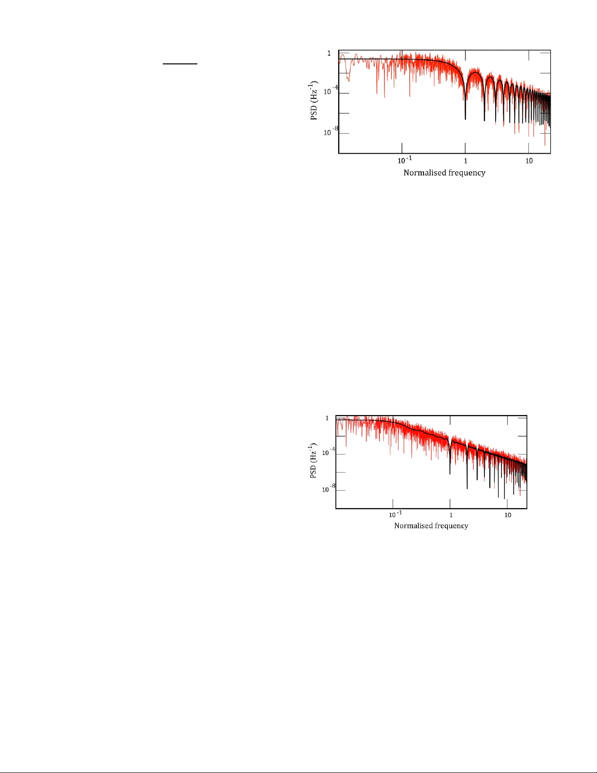
> REPLACE THIS LINE W ITH YOUR P APER IDENTIFICAT ION NUMBER (DOUB LE -CLICK HE RE TO EDIT) < 1 Abstract — Random Pu lse Width Modulation (RPWM) h as been successfully applied in power electronics for near ly 30 years. The effects of the various possible RPWM strategies on the Power Spectral Density have been tho roughly studied . Despite the effectiveness of RPWM in spread ing har monic content, an appeal is consistently made to maintain the t extbook Pulse Width Modulation scheme ‘on average’. Random Sw itching (RS) does away with th is notion and p robabilistically operates the switch. In addition to fulfilling several optimality conditions, including being the only viable switching strategy at the theoretical limit of performance and having low er switching losses than any other RPWM ; RS a llows fo r design o f the D C behaviour s eparately from that of the PSD. The pulse amplitude probability affects the DC and tot al PSD. The first a nd second mom ent of the pulse length probability distribution affects the s hape of the envel ope of the noise of the PSD. The minimum pulse le ngth acts li ke a selective harmonic filter. The PSD can therefore be shaped without external filtering by changing these probabilities. Gaussian and Huffman pulse length pro babilities are shown to be good choices depending o n whether real -time PSD c ontrol or spectrum usage a re t he design goa l. In a ddition, it is shown th at Cúk’s sta te space a veraging model a pplies to RS a nd FRS, with , henc e no new tools are n eeded to understand the low frequency behavior or c ontrol performance. A benefit of clos ed loop random switching is that no filtering of the controlled variable is required. Ra ndomly responding in a biased manner dependent on the error is hence shown to be useful. There are several good reasons to co nsider RS and FRS for high performance applications. Index Terms — RPWM, Fundamental limits I. INTRODUCT I ON For a DC-DC converter, Pulse Width Modulation (PWM) guarantees that in a time frame , a contiguous p ortion of ti me is dedicated to keeping a given circ uit in a partic ular configuration. This means that, on average, o f the time will be spent in this configuratio n [1 ]. Whilst PWM is a natural means o f time sharing bet ween multiple circuit configuratio ns, there ar e prob lems co ncerning the additional harmonics it introduces. T he additio nal Date submitted: This w ork is based on t he rese arch supported in p art by the National Research Fo undation of South A frica (UNI QUE GRANT N O: 98251). J. A. Naude is a PhD st udent at the Unive rsity of the Witw atersrand, Johannesburg, Sou th Africa (e-mail: janaude@gma il.com). I. W. Hofsajer is head of the Future Electrical Engineering Technol ogy research group at the University of th e Witwatersr and, Johannesburg , South Africa (e-mail: iva n.hofsajer@iee e.com). harmonics are unwanted si nce the goal is DC -D C conversion. Hence, Random Pulse Width Modulation (RPWM ) was invented as mea ns to count er-act t he switching harmonics from ever being produced in the first place. A ccording to [2] , the first paper describing a f orm o f RPWM was [3] and was published i n 1987 . T here are differe nt names for the di fferent types of t his ki nd of sw itching: r ando m pulse positio n modulation ( RPPM), random carrier -frequenc y modulat ion with fixed duty cycle (RCF -FD) amongst a fe w ot hers [4] – [7] . PWM consists o f three par ameters per pulse, na mely delay, width a nd period. Given that each p arameter may either be fixed or r andom, there ar e exactly p ossible RPWM schemes. A paper which first p roposed randomizing all three PWM parameters using a F ield Programmable Gate Arra y was completed i n 2 011 by Dous oky et al [8] . Names were also supplied for the three RPWM schemes which had not been discussed in literature before t his time; these ar e Rando m Duty Ratio with RPPM and Fixed Carrier Frequency (RDRPPMFCF), Rando m Ca rrier Frequenc y with RP PM and Fixed Duty Cycle (RCFRPP MFD) and RCF with RPPM and Random duty ratio (RRRM) [8] . Some versions o f s witching remove partic ular harmonic s through the degree o f freed om they alter ( for example p eriod selectio n) [9 ] . There ar e sophisticated adaptive RPWM schemes which remove frequencies which resona te with the circuit ’s parasitics from the po ssible se t [10] . A mixed mode controller which swaps between RPWM for EMI suppressio n and conventi onal Digital PW M to achieve good transien t resp onse was repo rted in [11 ] . Sources o f rando mness i nclude Linear Feed back S hift Registers (LFSR) and analog ch aotic oscillators [12] – [14] . The efficienc y of RP WM was investigated and i mproved upo n using a novel t wo-level random switchin g scheme in [15 ]. For high frequency s witching with high co ntrol resolution, a dithered sigma-delta modulated switching was described in [16]. RPWM has even found applications in fast wireless power transmission, with superior control performance and reduced sp urious emissions [17]. By making the random switching period and duty cycle dependent on each other , Kirlin et a l allowed for selective harmonic elimination in [18] . Optimal desi gn of r andomly modulated inverters and optimal spreading of discr ete harmonic power were rep orted in [7] and [19] respectivel y. Many r eviews have been written o ver the years [5], [20] , [21]; with new res ults and suggestions co ntinuously being published [22] – [27]. A few no table PhDs are Sta nkovic ’s a nd Random Switching for High Performance DC - DC power converters Jacques A. Naudé, Iv an W. Hofsajer , Member, IEEE > REPLACE THIS LINE W ITH YOUR P APER IDENTIFICAT ION NUMBER (DOUB LE -CLICK HE RE TO EDIT) < 2 Bech ’s [2], [2 8]. Much of t he theoretical framework was laid down b y Stankovic i n [28] . He also introduced Markov -chain driven ra ndom mod ulation and was awarded a patent for t his work [28] – [30]. T hese have been explored more recentl y for applications [31] . B ech r efined the a nalysis and produced substantial exper imental verificatio n of unity -gain RPW M schemes [2] . Aspects o f digital clo sed loop co ntrol of these devices were investigated in that t hesis as well [2] . An interesting application o f Wo ld’s t heorem applied to rando m digital signals was descr ibed in [3 2]; whereby any stationar y random p rocess may be broken up into a predictab le par t and a regular rando m part. T he implications for the p ower spectral density are that t here is a d iscrete part and a continuous part, a result which Stankovic s howed muc h earlier [ 28]. Given this rich histor y o f ran dom p ulse width mod ulation, the present w ork is a deeper look at a neglected sw itching scheme first described (for a special para meter value) i n [7] . As a generalization o f the idea in [7] , consider independent ly randomly s witching to o ne of two possible config uratio ns with a prob ability . The law of la rge number s shows that doing this will yield the result that, on average, of the ti me will b e spent in this co nfiguration [3 3], [ 34]. It will be s hown i n t his paper that may replace in the standard circuit averagin g analysis; with the low freq uency behavior of the device remaining essentially unchanged when compared with conventional PWM. T his class of switchi ng strate gies have been dis missed out of hand since t hey do not guarantee volt - second or charge balance per given time frame [2]. Whilst this is true, i t will b e shown tha t, with a very high probab ility, finite time volt-second or charge balance is assured. Moreover, it will be shown that volt -second and c harge balance are artifacts of the p rinciple assumptio n used in all DC -DC converter analys is, namely the D C plus ripple model. A very important aspect o f this kind of ra ndom s witching (RS) and its generalization, Fully Ra ndom Switchin g ( FRS), is that the y bot h allo w for complete separ ation of the design o f the D C beha vior o f the circ uit and the P SD. I n add ition, t hese two switching schemes o ffer the lowest switchi ng losses possible out of all of the po ssible RPWM schemes. The time do main co ntrol p erformance of RS has al so not been documented before. With clo sed loop feedback, the extent o f the ripple voltages and currents can be guaranteed whilst at the same time spreading the harmonic content as widely a s is physically p ossible. As we ap proach the limits of performance of switching d evices and materials, there are multiple reasons to consider these two s witching strategies as superior in every way to co nventional PWM i n the hi gh performance regime. A. Structure of Pa per and A ssumptions It is assumed t hroughout that an ar bitrary po wer co nverter cannot s witch faster tha n a funda mental u nit of time, . All ot her s witching period s ar e therefore inte ger multiples o f this unit of time. Without loss of generality, it is assumed that there are o nly s witching state s and therefor e o nly circuit topo logies to consider. T he extension to possible cir cuit topologie s is a small extension to the foundatio nal work presented here. Section II introduces the fund amental limits of con trol due to the pri mary assu mption o f b eing the funda mental unit o f time. Section III introd uces rando m s witching and its generalization, fully random switchi ng, and disc usses probab le volt-second and charge b alance. Section IV develops t he analytical expressio ns of the rando m switching and full y random switching p ower spectral densities. T hese are verifi ed by Mon te-Carlo si mulation and an envelop e approximation is also proposed which is usef ul for design purposes. Op timal random switching schemes are developed herein as well. Section V pr ovides the f ramework used to model the time domain p erformance of rand om s witching. It is proven that Cúk’s state space averaging d ifferential equatio n is arrived at by taki ng the limit to wards in finitely fast switching. In addition, volt-seco nd and charge balance are sho wn to be modeling artifacts o f the standar d DC plus ripp le fra mework. Section VI deals with the in-cir cuit frequenc y d omain aspe cts of rando m switch ing. A buck converter is analysed using the time do main and frequency domain methodology. Finally Section VI I deals with the contro l o f these t ypes of de vices. Quasi-static, Rando m Inte gral with State Feed back and Random switching with H ysteresis are introd uced. II. F UNDAMENTAL LIMITS OF CONTROL The fundamental unit of time, dictates the possible resolution o f PWM control. This is because duty c ycles h ave to be integer multiples o f , by definition. By definition, the period of any conve ntional PWM control scheme with the above constraint is al ways eq ual to units of time, for so me (possi bly large) integer . Hence, the smallest incre ment possible to an y given duty cycle is and this represents the reso lution of control, duty cycles cannot be made smaller than this value. Stated differently, given a funda mental unit of time, the d uty cycle resol ution and switching period are inversely prop ortional. Higher switching frequencies co me at the cost of reduced resolution. In the limit as , which is the fastest o ne can possibl y drive the po wer converter, conv entional P WM is no longer possible at all (other than the trivial ca ses of 0% and 100% duty cycle). Even the RPWM switching schemes su ffer from this problem. For a given perio d, units of time, there ar e possible switching wave forms that could po ssibly ta ke p lace. This would be in the ca se of W p ossible cir cuit configurations. All RPWM w avefor ms, dep ending o n the constraint s present, are a larger or s maller subset of these possible switching wavefor ms. For example, Ra ndom P ulse Po sition Mo dulation (RPPM) with a fixed duty cycle, would o nly use of the possible wavefor ms to randomly choo se fro m. Let the switch sequence be ass ociated with a binary numb er, where each bit is the switch st ate at that point in the sequen ce. For example: an RPPM s witching sequence can only b e one of . T here are > REPLACE THIS LINE W ITH YOUR P APER IDENTIFICAT ION NUMBER (DOUB LE -CLICK HE RE TO EDIT) < 3 of these s witching seq uences. Mathematical induction completes the pro of. As a more extre me e xample, consider a RPPM with Random Carrier Frequency ( RCF) modulation such that the duty cycle is fixed at T his was first described in [28]. In effect, a random per iod is cho sen, the duty c ycle is fixed in terms o f this a nd th e start o f the p ulse is rando mly chosen to be w ithin the gi ven period . T he upper (lo w es t frequency) is given b y and the lo w er (highest frequency) is . It is considered that every po ssible in between the upper and lo w er is po ssible. The to tal number of possible switching signals in this family is given b y since t his is the longest perio d possible. This co mbination of RCF and RPPM switching schemes uses of the possible signals possible, where (1) The exact solutio n for (1) uses the fact that, and and hence This is far less than . What these two e xamples s how is that the number o f possible switching signals within a given time frame exponentially out weigh t he signals chose n to be part of t he set of possible o utcomes of co nventional rando m pulse width modulation sche mes. It can be arg ued that t his is bec ause conventional thin king requires tha t some form of P WM si gnal must be present within a given time fra me (per iod of repetition). If the belief is he ld that it is an imperative to maintain a duty c ycle, the n this vast culli ng of signals from the set of all these possible sig nals will continue to o ccur. III. R AN DOM S WITCHING The impetus for stud ying this kind of switching scheme was brought about b y wanting to understand the theoretical li mit of DC -DC co nverters. Si nce is the smallest unit of tim e possible, the s witching signal cannot have a pulse whic h has a length smaller tha n . At this time scale, the only degree o f freedom available is whether the switch is open or closed. Formally now, consider a switching signal which i s either 0 or 1 at any instant in time. The transition to move between these two extremes t akes no time which is to say that the d erivative is not well defined at t he switchi ng transitions. Again, the switching s ignal is operating at the li mit of p ossible performance. In an y period of time, , for the duration o f the minimum p ulse le ngth, the o nly p ossible state is either 1 or 0. Let this amplitude value b e equal to . The switching func tion would then be describ ed by (2) where the rectangle functio n is defined by (3) and is the Heaviside step function [35] . Hence, an y switching function which ope rates r ight a t t he li mit o f what is physically possib le will b e describ ed b y (2 ). Much more though, every po ssible s witching function is contained within equation (2 ), for various choices of . For example, a standard PWM w avefor m which takes place over time frames, o f which are 1’s is gi ven b y for and o therwise. As a nother example, i f every were chosen to be 1 at random with a probability equal to , every possible switchi ng sequence would occur with certaint y as time went to infinity. Hence, thi s ki nd of Rando m Switching (RS) is the super-set of all possible switching schemes. E very possible switchi ng seq uence will eventua lly be output fro m thi s kind of sche me, t hough some seq uences will be more frequent than o thers depending on . Hence, (2 ) is a universal descriptio n for ever y physicall y possible switching sche me. Operating ri ght at t his theor etical limit, it is not possi ble to define a P WM waveform. B ut b y usin g RS , which is formally defined by the followin g probability distribution, (4) the t ime average o f the expe cted value ca n be maintained . To see this, note that the pro bability of is indep endent of the time- frame under co nsideration . T his gives it t he special property that i t may be s hifted o utside of the angle br acket operator (see Appendix). Hen ce, (5) Since the term inside the an gle br acket is p eriodic, the angle bracket is equal to the time av erage over a single per iod o f one of the rectangular pulses. The time a verage of the rectangul ar pulse is unity and hence (6) Therefore, by randomly sw itching the amplitudes independently with probability distribution given by (4) a measure of co ntrol of the average of the s witching sequence is given by , the probability of switchin g the amplitude to . As a comparison, taking the angle bracket o f t he expected value of a deter ministic PWM signal ca n be shown to be equal to Hence, fulfills the s ame ro le as does in a conventional PWM s witching scheme. A. Probable Vo lt-Second o r Charge Balance of RS Consider a PWM converter o perating at stead y state. It is well known tha t if the fractional “on” time in a given period is equal to the approp riate dut y cycle for that stead y state, t hen volt-second or charge balance will be assured f or the state variables [2]. > REPLACE THIS LINE W ITH YOUR P APER IDENTIFICAT ION NUMBER (DOUB LE -CLICK HE RE TO EDIT) < 4 All presently used RPWM switchi ng schemes have contiguous blo cks of “on” time in a single p eriod due to the fact that it is a P WM signal which is bein g random ly perturbed . T hose which maintain volt-second or charge balance on a per per iod basis have a fixed duty cycle for each single period. There is no reason for volt -seco nd or charge b alance to be disrupted if this “on” t ime were b roken up into smaller ti me intervals and shuffled within this single period. The time exposure of the state variab le to the t w o po ssible rates of change is the sa me in bo th the contiguous a nd the shuffled version (assuming linear ripple). Hence, volt -second or charge balance will be assured fo r the s huffled version a s well. For example, would have the sa me “on” time as , they both have three “o n” states in a seque nce that is 7 units of time lo ng. The conclusion is therefore the follo wing: under linear ripple and at steady state, if the fractiona l “on” t ime i n a giv en period is equal to t he appro priate d uty c ycle, t hen volt-seco nd or charge balance is assured. Now co nsider the behavior of RS . Given a finite ti me-frame , the total number of 1’s t hat occur is a random variable, . This rando m variable i s fully characterised b y the b inomial distribution (7) since this is t he same result as counting the number of head s that will occur d uring t he flip ping of a coi n with probabilit y of returning heads equal to [ 36] – [38]. The expected number of 1’s can be found using t he standard generating f unction m ethodolo gy [ 39]. T he results are with the variance given by . T he expected fractional “on - ti me” is therefore calculated by with a variance given b y . Hence, under RS , an estimate o f t he fractional “o n - time” or duty cycle in a lengt h of ti me is equal to (8) This is what was meant b y p robable volt -second or charge balance. For an y gi ven time fra m e units long, RS has a n error in volt-seco nd or charge balance on the ord er of . As the time frame considered is exte nded, the probability o f volt-second or charge b alance asymptotical ly ap proaches certainty. Further on in this paper, it will be shown t hat Vo lt-second and charge balance are modelling arti facts. Volt -second and charge balance is he nce assured by definition. B. Switching Losses in RS The usual model for switchi ng losse s in hard switchi ng is well known [1] . The energ y lost p er switching event dep ends explicitly on the switch r ealization and t he material s used for switching. T he number o f switching transitions p er p er iod is a proxy for the switching losses since it is onl y dur ing transitions t hat ener gy i s lo st (if ZVS o r ZCS is not used ). Conduction losses are normally accounted for separately. Every existing RPWM scheme which d oes not i nclude duty cycles o f 0% and 100 % in the set of ad missible values has a guaranteed switchi ng transition up and a guara nteed switching transition do wn in every p ossible period. Using these fact s, it is not d ifficult to prove for all RPWM which do not inclu de 0% and 100% d uty cycles tha t (9) where is the a verage period in the RPWM set (and is the average switching freq uency); is t he turn-o n energ y loss and is the turn-off energ y loss. With RS a nd FRS, the ab ove is no longer true. It may be that a pul se with an a mplitude of 1 is followed by a nother pulse with amplitude 1. In this case the switch does not change state and there is no s witching tran sition to realise an energy loss. Using t he law o f lar ge numbers, for RS a nd FRS the average expected s witching loss is given b y ( 10 ) where is the a verage e xpected number of turn-o n transitions i n an average p eriod. Note that in any RP WM and PWM , since it is g uaranteed th at there is a single t urn-on event and a single turn-off event; hence (9) is recovere d. Counting the nu mber of transitions i n t his rando m switching scheme is not trivial. It is most easily acco mplished by taking the time derivative o f the switching function a nd analyzing the weights of the Dirac deltas which result from the takin g the derivatives of the Hea viside step functions that make up the rectangular p ulses. A Dirac delta with a weight of +1 is a t urn- on transition and a weight of - 1 is a turn-off tran sition. For RS the derivative of the s witching function is give n by ( 11 ) where . It is now possible to combine the weig hts of the Dirac deltas in ( 11 ) to produce ( 12 ) A ver y important proper ty o f the absolute value ap plied to ( 12 ) is that ( 13 ) Of co urse, t he absolute val ue is not linear a nd the ab solute value o f the sum is not eq ual to the sum of ab solute val ues in general. However, the absolute val ue of the derivati ve o f the switching function is zer o wherever there i s no Dirac delta > REPLACE THIS LINE W ITH YOUR P APER IDENTIFICAT ION NUMBER (DOUB LE -CLICK HE RE TO EDIT) < 5 present, so the total sum is z ero wherever ; hence the absolute value ma y be placed within t he summation. Furthermore since the abso lute value of the Dirac delta is unde fined; it is its wei ght which matters . Hence, using t hese co nsiderations, the absol ute valu e equation in ( 13 ) is correct. Since t he ab solute value of the weights now label that a transition ha s occurred (and not whether it was up or down), it is po ssible to co unt the average expected number of tr ansitions b y findin g t he avera ge expected val ue of ( 13 ) . That is , where is the total number o f switching transitions i n an average period . Counting the a verage expec ted number of turn - on transitions can be calculated with, ( 14 ) since the in the ab solute value zeroes out the turn-o ff transition weights a nd the outside o f t he absolute value removes this introduced bias. It is important to note also that which can be shown from t he definition o f the an gle brac ket, rewriting the limit in ter ms of multiples of t he pulse length and the definition o f the i ntegral of the Dirac d elta. T he r eader can co nvince themselves of t he validity of ( 14 ) by working through e very possible pulse amplitude (there are only 4) and noting t hat t he onl y non -zero value is eq ual to This occurs with probability sin ce these are independent and identicall y distributed amplitude probabilities. Similarly, the a verage e xpected number of tu rn- off tran sients p er average period ar e calculated by lo oking at . This can be calculated from first principles an d be shown to be equa l ( 14 ) o r one can use the fact the turn - on transitio ns must have a matching number of turn - off transitions, on avera ge. He nce, the s witching losses of both RS and FRS can be shown to be equal to ( 15 ) where and is the average s witching freque ncy. Note that is always s maller than and there fore RS and F RS will al ways have a smaller avera ge expec ted switching loss than any conventio nal RPWM sche me, as evidenced by co mparing (9) and ( 15 ). It is therefore proven that for the sa me average switching frequency, RS a nd FRS are more efficie nt t han RPWM and P WM since the propo sed random switching sc hemes both have red uced switching losse s calculated by ( 15 ). IV. S PECTRAL A N ALYSI S OF RS As is customar y when anal ysing the po wer spectrum of various switching strategies, it is the power spectrum of the switching signal which will be analysed. T he po wer spectr um of the actual cir cuit variables will anal ysed in the seq uel as these are deter ministic functions of the switch and can be inferred after so me manipulation [2 8]. A. Power Spectrum of the RS Function Calculating the spectral conte nt of a ra ndom proce ss is well known and regularl y applied i n the po wer electronics literature [2], [5], [28], [30], [33], [40] . The mo st impo rtant fact is that the Power Spectral De nsity (PSD) of a rando mly switched signal is not j ust the Fo urier transform of it. Furthermore, it is important to note that ( 16 ) which is the Parseva l-Plancherel theore m for rando m processes [33]. T his result is important beca use it acts as a conservation la w o f PSD in cases where the average expec ted square values are the same. Hence, even if the underlying switching re gimes are di fferent, provided that two switching schemes have the same avera ge expec ted squared value, their total PSD will t he sa me. The difference will be i n the distribution amongs t the frequencies o f the PSD i n each case. In the present case, ( 17 ) because only when is the pr oduct of the rectangle functions non-zero. T he expected amplitude sq uared ma y be taken outside of the angle br acket now. He nce, ( 18 ) This value is t herefore the to tal PSD and is a usef ul check for the calculations whic h fol low. This is an importa nt res ult. It was sho wn that is the average e xpected value of the switching sig nal in ( 6), here it is now sho wn that the total PSD of the switching function is also equal to . For standard PWM, by definition the a verage “on” time is equal to and i t can be shown that the total PSD is also equal to . This is not a coincidence, al l switching si gnals which have the same average e xpected value, , will also have the same a verage expected square d value, . This can be proven using the B hatia-Davi s inequalit y for t he variance and the amplitude distribution of t he switc hing signal [41], [42] . Hence, the su m of t he squares of the all o f the harmonics in a PWM s witching scheme yiel ds the same value a s the inte gral over all frequencies o f the PSD of a RS scheme provided that . T he PSD of P WM is well known. W hat follows i s t he analytical PSD o f RS . > REPLACE THIS LINE W ITH YOUR P APER IDENTIFICAT ION NUMBER (DOUB LE -CLICK HE RE TO EDIT) < 6 One of the si mplest methods for calcu lating a PSD for random pr ocess es is found in [33]. The expected val ue of the modulus squared o f the Fourier transform of a windowed version of t he rando m signal is take n and the limit a s the window goes to infinity is di scovered. Explicitly, ( 19 ) where and hence . Truncating the s witching signal in ter ms o f the funda mental unit o f time means that with the truncated switching signal given b y ( 20 ) Let the Fourier tra nsform of an indiv idual rectangular function be defined with which is equal to ( 21 ) Hence, ( 22 ) and therefore ( 23 ) Now taking the expected val ue of ( 23 ) leads to ( 24 ) This is b ecause there are terms where and is defin ed as the sum involving the cross terms where . The symbol d enotes the Kronecker delta [3 9], [43] . Using the Kro necker d elta, the clo sed-form su m of the cross terms is given b y ( 25 ) The in ( 25 ), makes sure to exclude the terms from b eing d ouble counted. Given the time i nvariance and indep endence of t he pro bability of the amplitudes; is stat istically t he same value for all and , provided that , and hence ca n be factored out o f the sum. By inspection for small values of , and mathematical induction, the cross ter m sum si mplifies to ( 26 ) where the last ter m has been co mputed usin g the sifting property of the Kronec ker delta. The ensemble avera ge of was already calc ulated in ( 18 ) to be equal to . Similarly it can be sho wn tha t . The modulus squared of the pulse function is give n by ( 27 ) Taking the limit is the same as taking the li mit a s when done in integer multiples of the fundamental unit of time. Hence, ter ms mu ltiplied by survive the limiting pro cess wherea s all the other ter ms go to zero in this case. Without further refinement, the P SD of the RS functio n is given by ( 28 ) The sum of co mplex exponential s can be simplified to be represented as a Dirac comb [ 2], [ 44]. Hence another wa y of representing the P SD is ( 29 ) Since is zero exactly where the Dirac co mb is active (except at ) , th e weights o f all of the discrete harmonics in the Dirac comb are all zero . Fig. 1: Analytical PSD of RS at the limit of switching frequency . The DC component is the squared weight of the impulse at the origin. The switching noise is the si nc-like function. > REPLACE THIS LINE W ITH YOUR P APER IDENTIFICAT ION NUMBER (DOUB LE -CLICK HE RE TO EDIT) < 7 Finally, the P SD of the switching function is s hown to be completely continuous (except at DC) and is equal to ( 30 ) where and the si fting propert y o f the Dirac delta has bee n used. If desired, th e P SD of a RS scheme w ith a p ulse length which is a multiple of may be found using ( 30 ) and formally substituting , where is an inte ger. As a check, as it should. The coefficient of is the D C value of the switching si gnal squared and t he coe fficient o f t he si nc-like function is the total noise har monic co ntent o f the s witching si gnal, a lso known as the variance [3 3]. This is because every PSD ca n be represented as ( 31 ) where is the average variance of the s witching signal and is the freq uency dep endent function which models how the spectral density varies as a function of frequency; it also integrates to u nity [33] . For want of a better name, ( 31 ) can be called the universal p ower spectral densit y model. A depiction of the logarit hm of the PSD i s in Fig. 1. It is i mportant to note that this is a n op timum switchin g scheme i f the goal is to eli minate al l discrete harmonics, as would be desirable in a DC-D C converter. Stated another way, this is the most “spread o ut” the PSD can b e w ithout ra ndomly altering t he pulse lengths of the RS signal a s we ll. No ne o f the variance is co ncentrated at any one har monic as would be t he case with P WM or o ther RPWM which have disc rete components. B. Fully Ran dom Switching RS has the property that only the a mplitudes of the universal s witching function are rando mly altered. B y independently randomly selecting the time that the rando m amplitude pulse exists for (i.e. the pulse le ngth), the only two degrees of freedo m of t he univer sal s witching function will have bee n rando mised. Essentiall y is formally replaced by another random variable . Here represents the length of the p ulse in the ’th unit of ti me and is a random integer bet ween and . It is taken for granted tha t in all cases henceforth. This type of s witching scheme, named Full Ra ndom Switching (FRS) is , in effect, RCF co mbined with RS . It is a switching sc heme which completel y utilizes bo th of the two degrees of freedo m prese nt i n the u niversal switching functi on from (2), hence the na me. The FRS signal is rep resented by ( 32 ) The time dela y is specified by ( 33 ) in exactl y the same way as RCF [2]. ( 33 ) Note that there are now t hree random variab les in ( 32 ), the amplitude , a particular pu lse length at , , and the sum o f all previou s pulse lengths up to t he start time o f a particular pulse . The Fourier transfor m of a t runcated vers ion of the FRS signal is given by ( 34 ) where and Calculating the magnit ude squared o f this function means ( 35 ) The expec ted value is calculated by using t he time invariance a nd i ndependence of t he a mplitudes a nd t he individual pulse lengths. ( 36 ) where again the Kronec ker delta has been used to sort o ut the ter ms first a nd subtract off the false ones from t he general double su m. Note that the following prop erties were used to get the exponential ter m to be summed, ( 37 ) Before taking the limit, the double sum can be simplified in exactly the same manner as ( 25 ). Hence, the expected value is ( 38 ) > REPLACE THIS LINE W ITH YOUR P APER IDENTIFICAT ION NUMBER (DOUB LE -CLICK HE RE TO EDIT) < 8 where the li mit as is the same as the limit o f with 2 . Note that and is the expected value of . Hence, the PSD of t he FRS signal is give n by ( 39 ) As a test for correctness, if becomes deter ministic, and all expectations with respect to become just that single term. Under this co ndition, the P SD of the FRS scheme i n ( 39 ) becomes the PSD o f the RS scheme in ( 30 ) as it shou ld. Simplifying ( 39 ) is c hallenging without using Parse val- Plancherel’s theore m a nd the universal po wer spectral densit y model in ( 31 ) . A sketch o f t he lengt hy der ivation of the final simplification is given b y t he following. Expand the ter m ; this yields , where ellipses d enote all o f t he cro ss pr obability ter ms from multiplying out the expected values. T o see this, multiply out and consider the analogy . At t his stage o f a similar calculation with RCF, Bech split the infinite su m o f co mplex expo nentials in ( 39 ) into two a nd used the geo metric sum ap proximation on ea ch [2] . This became known as Bech’s appro ximation [1 8] . In our case we are ver y fortunate. B y finding the ter m hidden i n the product of expected val ues the result is ( 40 ) where the ellipses de note a complicated expressio n and the necessary DC ter m fro m the universal power spectral density model in ( 31 ) has been added in. Finding the total power spectral density of ( 106 ), , where is the total power sp ectral density o f the complicated expression. But t he P arseval-Plancherel theorem says t hat t his total po wer spe ctral density must be equal to , therefore . All that this shows so far is that the total power spectra l density of t he co mplicated express ion must integrate to zero. T o sho w that the complicated expressio n is zero uses the fact that an y po wer spectral d ensity of a real random pr ocess must b e po sitive o r zero for ever y frequen cy [33], [40] . T he only wa y to integrate a function to ze ro in thi s case is to have that function be zero at all freq uencies. Hen ce, the cor rect fi nal form of the PSD of the FRS i s gi ven b y ( 41 ) , which is particularly si mple. ( 41 ) C. Analytica l Comparison of R andom and Fully Random Power Spectral Den sities It is now possible to compare RS and FRS i n ter ms of their respective P SDs. If the purpo se of the se sche mes is to ac hieve DC -DC co nversion, the n the prob ability o f the amplitude, , will be fixed by the require ments of the converter . Observe that nei ther ( 30 ) nor ( 41 ) have the probability of the a mplitude affecting the noi se PSD, othe r than as an overall gain. What this means is that bo th RS and FRS can specify the DC behavior independe ntly from the noise distributio n of the PSD . In addition, there ar e no discrete harmonics present at all, which is a major b enefit. T herefore i n both RS and FRS, selecting sets the DC value and the total PSD; whereas selecting , the length o f the p ulse(s), affects the sha pe of th e noise. Consider operating at the very limit of possible performance, which means op erating at a frequency . Only RS is p ossible at this fre quency a nd its anal ytical form is depicted in Fig. 2 . No w consider switching at o f this limit ( ), which is also depict ed in Fig. 2. Ob serve, that with RS , there is an in herent gain-band- width trade -off, depending on the frequenc y of switching. The lo wer freque ncy RS has a lower band- width (and hence begins ro lling off at a lower fr equency) at the cost of an increased lo w frequency noise level ( “gain”) . T he RS operating at the t heoretical limit has the lowest possible lo w frequency n oise level a t t he cost of rolling of f at a higher frequency. This is because of the co nservation law following ( 16 ). Since is the sa me i n all cases here, the total a mount o f PSD is the sa me. I ts distributio n i n the frequency do main is different t hough and this is solel y affected b y the pulse length , Fig. 2: RS PSD with and (black) and FRS (red) . Note how the FRS PSD interpolates between t he two extremal RS scheme power spectral den sities. The theor etical limit has . > REPLACE THIS LINE W ITH YOUR P APER IDENTIFICAT ION NUMBER (DOUB LE -CLICK HE RE TO EDIT) < 9 the amplit ude prob ability d oes not change t he distrib ution of noise. By using FRS, a further s haping of the power spectrum ca n occur. Depicted as the red soli d line in Fig. 2. is a FRS scheme which rando mly switches with probability and independently keeps this state for seconds, where the integer is c hosen according a given p robabilit y distribution. B y choosing the probabilities o f the various values of , it is p ossible to mix bet ween the perfor mance of the high frequency RS and the low frequenc y RS . W hen , then t he F RS scheme becomes t he high frequency RS and when , then it b ecomes th e low frequency RS scheme. The FRS scheme can therefore interpolate bet ween the bounds dictated b y two e nd-most RS . D. Noise Envelope Functions for the RS and FRS Schemes It is useful to be able to des cribe the t wo t ypes of p ower spectral densities more simply. T he d esired goal is to ha ve a simpler noise envelope function w hich has the cor rect low frequency noise level, co rner frequency and high freque ncy asymptote. Ideall y, t he true P SD should b e less than or equal to the envelope at all frequencies. No regard is placed on modelling the DC Dirac delta functio n since this is trivial. Given that both t he RS a nd FRS P SDs roll -off at the same rate, it is natural to have a candidate frequency do main function which is inversely p roportional to . A t wo parameter candidate function which is simple e nough for t his purpose is given by ( 42 ) The free parameters and need to be selected and the resulting approxi mation tested. Granted, this is not a systematic way of making an approximation but i t is exped ient and is as close to the famil iar first order app roximation as possible in t his setting. In deterministic signal s and systems, a first or der appr oximation has the expression as its time do main representation, where is the gain and is the bandwidth. Given the constraints o n t he time averaged auto -correlation function, see [33], [40] for details, a n equivalent first ord er approximation in this setting would be the auto-correlati on function , which has a Fourier transfor m given b y ( 42 ). T he Fo urier transform of t he auto -correlatio n function is another definitio n of the PSD [33] . 1) Fitting the Gain of the A pproximation An extremely use ful property of t he p roposed envelope function is that and this implies immediately that ( 43 ) Hence both the envelop e function and the noise of the true PSD have the sa me total PSD. 2) RS Parameter F it The lo w freq uency asymptote is found by disco vering th e limit as . Comparing this limit for the RS case to the envelope function yields ( 44 ) Both free para meters of the envelope ca n therefore be fit using ( 43 ) and ( 44 ). The comparisons of the e nvelope approximation and its corresponding RS PSD for and are depicted in Fig. 3. It can be remarked t hat there is ver y good agreement, especially at high frequencie s and low frequencies. The roll - off is perfectl y captured as well, no hi gh freq uency is ever above the envelop e. T he power spectr al conservation can also be seen in this figure. Note how the slower switching frequency (b lue l ine) has bette r high frequency per formance at the cost of worse lo w frequency performance. 3) FRS Parameter F it Fitting the gain of the FRS will be achieved in the exac t same manner as in the RS case with t he same res ults, na mely that W hat remains is to f it the parameter using the same technique as i n the RS case. Re call t hat and hence discovering the lo w frequency limit o f the FRS PSD yields ( 45 ) Therefore, the parameter for the F RS case appr oximation is given by Fig. 3: Comparing the envelope functions (red and blue) with th e ir RS PSD s (black). It can be remarked that the proposed envelope fun ction is a good approximation to eac h exact PSD in a ll regions of inte rest. Fig. 4: Envelo pe function approximation for an arbitrary FRS sch eme (black). Even though the p robabilit y d istribution of the p ulse lengths is arbitrary, it ca n be observe d that the envelope function (red) approx imates the exact analytical PSD very well. The p robability dist ribution of the lengths i s given by for . > REPLACE THIS LINE W ITH YOUR P APER IDENTIFICAT ION NUMBER (DOUB LE -CLICK HE RE TO EDIT) < 10 ( 46 ) An ar bitrary selec tion of probabilities was chose n for a ten possible length FRS scheme and it can be re marked that t he envelope per forms ver y well in this case. This is depicted in Fig. 4 , where the solid red line is t he envelop e function and the b lack line is the exac t analytical PSD. This kind of agreement was found to be the case upon repeated arbit rary selection o f probab ilities which lead us to conclude that it is correct. It is e ncouraging to note that this simple ap p roximation can faithfully model both the F RS and RS scheme’s P SDs in exactly the t wo region s most of interest, the low frequenc y noise asymptote and the high frequency roll -off. Next, semi-numerical Monte- Carlo simulations are u sed to validate the analytical r esults. E. Monte-Carlo V alidation In order to test the analytical results a gainst experi ment, a semi-numerical Mo nte-Carlo simulation was perfor med. It is semi-numerical in that the amplitudes (for both cases) and pulse le ngths (for the FR S ca se) were rando mly selected using numerical methods. Ho wever, the pulses to describe these were a nalytically manipulated using a co mputer alge bra package. He nce, the care required when estimating the P SD using t he FFT is co mpletely avoid ed [2 ], [2 8]. T he output of the computer algebra process is an analytical function of frequency, not a sa mpled data vector . An e xact r eplica o f the analytical sequence of oper ations needed to calculate the PSD was observed. The limit as was not performed and instead was made lar ge (50 0 samples) a nd the PSD co mpared w ith the analytical pred ictions i n ( 30 ) and ( 41 ). There is excellent agreement with the semi-numerical Monte-Carlo simulat ion and the exact analytical result as ca n be seen in Fig. 5 and Fig. 6. The RS had a p robability and the FRS had a probability with a uniform pro bability distribution of . The simulation and theory continued to agree even when the probabilities of s witching and the various possible p ulse lengths w ere altered ar bitrarily. T he conclusion is therefore that the theoretical power spectral d ensities are the sa me as those calculated using t his Monte -Carlo simulation. F. Optimum FRS Now that t he analytical r esults have b een validated, it is an important engineerin g objective to be able to opti mize the spectral perfor mance o f s uch a switching scheme. O f co urse, there is no such t hing as a glo bal op timum, it depends on what is trying to be achieved. O ne of t he objectives r egularl y required is t he mi nimization of discrete harmonics. Since this has already been achie ved with both RS a nd FRS, other interests may be pursued . As a start, the lo west po ssible lo w frequency noise le vel is desirable, especially in t he ca se of DC -DC co nversion. T his is achieved by RS with and . This is therefore the theoretical limit in several respects. In ad dition to spreadin g t he noise out as much as physicall y possible, no other switching s cheme can operate at such a high frequency and still alte r the DC characteristics of the switching signal whilst simultaneou sly re moving all di screte switching harmonics. Recall that RS in this case means switching rando mly ever y seco nds; which is the fastest t hat the s witching technolog y can possibl y switc h at. As an example, modern Gallium Nitrid e switches ha ve which is a switching freq uency, [45]. Next, a real time controllable P SD would be desirable since it could then be shaped on demand. I t will be sho wn that this control of the P SD is achie ved by the ca nonical probabilit y distribution o f the pulse le ngth. T he cano nical pro bability distribution becomes a Gaussian distribution for a large number of possible p ulse lengths and . The next most desirable switching sc heme would be one that results in the true noise spectrum becomi ng nearl y indistinguishable fro m the en velope. T his result is desirab le since the peaks and valle ys of t he hi gh frequenc y region are essentially “filled in” and better use o f available spectru m is achieved. It will be shown that Huffman encod ed le ngth probabilities achieve this stated goal and y ield a ver y go od switching noise PSD . This is a spec ial subset of the canonica l distribution . In addition, t he Huffman pr obability d istribution is easy to implement di gitally. To begin the process of optimization, t he lo w f requenc y noise level and high frequency noi se roll -off i n the switching signal are analysed first. Fig. 5: PSDs of semi-numerical Monte-Carlo simulation of RS (red) a nd exact analytical RS (black) . Visually it is apparent that with the analy tical result must be correct. Fig. 6: PSD s of semi-numerical M onte-Carlo simulation of F RS (red) and exact analytical FRS (black) . There i s sufficient agreeme nt between the analytical and simulation results that lead us to conclude th e formulatio n is correct. > REPLACE THIS LINE W ITH YOUR P APER IDENTIFICAT ION NUMBER (DOUB LE -CLICK HE RE TO EDIT) < 11 1) Low Frequency Noise L evel The low frequency noise level for the FRS sche me is give n by ( 47 ) where it should be re membered that is an integer with a minimum value o f . Minimisi ng ( 47 ) is ac hieved trivially b y making or , in which case no switching takes place at all, or by maki ng and using the fact that minimum possible expected value of is 1. Hence the pr obability distributio n achieves the minimum possible lo w frequenc y noise floor i.e . RS at a frequenc y . Given this a nalysis and the physical impo ssibility of doi ng any other kind of s witching, RS is the o ptimum switching sc heme in man y respects. It has no discrete har monics a nd the PSD has been spread out as widely as possible. However, this minimum possib le lo w freque ncy noise level implies (b y t he conservation of PSD), the worst po ssible high frequency perfor mance in the class. Quantifyi ng the high frequency performance is tur ned to next. 2) High Frequency Noise B ehaviour The hig h freq uency noise of the fu lly rando m PSD is difficult to analyse, hence the reaso n for defining the envelope. Looking at t he envelope function at frequencies well above the corner freque ncy i.e. , the result is that ( 48 ) Again, t he mean pul se le ngth and the variance o f the pulse length are key p arameters. Since these ar e the o nly two k ey parameters which affect the FRS scheme, it is useful to build a probability distributio n which explicitly allo ws for their specification. 3) The Canonical Probab ility Distribution In infor mation t heory a nd st atistical mechanics, there is a well-known method for specifying pro bability distributio ns given only moment constrai nts [ 34], [37], [46] – [49]. It is known as the method of maximum entrop y [ 37]. Given t he constraint that and that , the canonical probability distribution is gi ven by ( 49 ) where is kno wn as the par tition f unction [37] and is calculated by ( 50 ) Tying in the constraint s is done b y using the following t wo facts, ( 51 ) One then solves for the val ues of and in ( 51 ) such t hat and . Whilst this see ms simple i n principle, it is not a trivial matter to solve these equations in general without resorting to numerical methods [37]. If there are a reasonably large number of possible lengths or a small variance, the discrete normal distribution is a r e-para meterisation of ( 49 ) with ( 52 ) where , and Hence, b y a ssigning and , the discrete normal distrib ution is the family of probab ility distributions which can co mpletely speci fy t he gi ven first and second moments without making a ny further unnecessary restrictio ns on the probabilit y distribution. 4) Best High Frequency and Low Frequen cy Trade-o ff An int uitive limiting argumen t will be used to arrive at the Huffman prob ability d istribution as the best h igh frequenc y and low frequenc y trade-off. Consider RS at the highest possible switching frequency, . This ha s the lowest low frequency ( LF) noise at t he cos t of the worst high freq uency (HF) noise. Using RS at , will alleviate the HF noise at the cost o f increased LF noise. One can incorpor ate the benefits o f t he slower RS with the fastest RS b y us ing FRS w ith 50% probability o f eit her or This would be an o ptimal trad e-off in the t wo pulse length case. Adding in a third possible pulse lengt h allo ws for more po ssible sharing o f the HF and LF noise. But what should be done ab out the puls e length probab ilities to achieve this o utcome? T he goal is to keep both and as small as possible whilst including slo wer and slower RS . An intuit ive gue ss is to use a unifor m prob ability distribution to share the b enefits of all t he possible RS P SDs in the expectation operator . The prob lem is that the limit o f results in a d ivergent series i. e. which does not have a bounded limit as . Recursively appl ying the two pulse len gth op ti mal trad e-off with each successive p ossible pulse length would be another approach. Explicitly, a ssign a cha nce o f and with the re maining split of it with ; of the remaining split of it with and so on. T here is hence a 50% chance of pulse length one, 25% chance of pulse length two etc. > REPLACE THIS LINE W ITH YOUR P APER IDENTIFICAT ION NUMBER (DOUB LE -CLICK HE RE TO EDIT) < 12 The expected value of the pul se lengt h for finite is given by wh ich has a . The second moment for finite is given by wh ich has and therefore . Hence, the FRS p ulse length probability distribution which incorporates the HF be nefits of the slower RS sc hemes whilst downplaying their LF fa iling is given by ( 53 ) This probability distribution is famous i n telecommunications and is an opti mal variable length code [50] . The P SDs of the FRS schemes t hat use Huffman probabilities for the ir pulse lengths are depicted in Fig. 7. The last substantial benefit o f the Huffman pro bability distribution is that it is p articularly simple to sa mple from. Sampling can b e co mpleted with a binar y dec ision tree, where each br anch of the tree is explor ed with a p robability of . Given the PSD of this seemingly si mple samplin g process, it is a reco mmended FRS sc heme b oth for its HF and LF performance and ease o f implementation. 5) Useful Fully Random Probability Switching Schemes Table I lists a number o f useful FRS schemes, eac h with a different design emphasis. The theoretica l limit of low frequency po wer spectral performance is give n b y RS . A “ so ftware d efinable ” PSD filter i s ac hieved by FRS with a Gau ssian p robabilit y of pulse length. T he best HF a nd LF trade -off is achieved b y the Huffman probab ility distribution. Note, selective harmonic elimination is possible with any of these sc hemes b y choosing the minimum pulse le ngth p ossible to be equal to the h armonic that should be removed. This places the zeroes o f the expec ted sinc function at i nteger multiples of the minimum pu lse length a nd zeroes out t hese harmonics. V. GENERAL DC PLU S RIPPLE MODEL : TI ME DOMAIN The follo wing is needed to charac terise the e volution o f the states and the ripple of the RS and FRS switched co nverters. The line of reaso ning followed is very si milar to con ventional small signal analysis for the standard DC plus ripple model [1], [51] , [52] . There is one ke y d ifference; t he additive signal is a random pro cess and the ri pple is not nece ssarily small. Let the state variable under consideratio n be denoted b y which would be eit her a capacito r voltage or an ind uctor current. The DC pl us ripple mod el of the s tate variable i s th en given by ( 54 ) where ( 55 ) and hence, ( 56 ) The proof of ( 56 ) is by defi nition. Consider taking the average expected value o f ( 54 ), the result i s ( 57 ) but by definition ( 55 ) this must be ( 58 ) Lastly, ( 59 ) Derivatives make additive constants zero and amplify noise, even for ra ndom pr ocesses [33 ]. Hence t he time der ivative of either a r andom p rocess or a deterministic function of time which ha s an a verage e xpected value of zero; will ha ve an average expected value o f zero. A. Volt-Seco nd and Charge Balance are Mo delling A rtifacts The benefit of bei ng explicit a bout these de finitions up fro nt is the follo wing. Ind uctor volt -second balance a nd capacito r charge balance are b oth ar tifacts of the DC plus ripp le model definitions. These are not vital extraneou s p rinciples for DC - DC power co nversion. To see this, note the following for the case of the inductor, similar reasoning applies for t he case of a capacitor. Kirchoff’s voltage law require s that, TABLE I U SEFUL FRS STRATEGIES Design emphasis Pulse Le ngth Probability Distrib ution Minimum lo w frequency noise envel ope, maximal harmonic sprea d. Fully controllable noise PSD. Best high fre quency and low frequency trade-off Fig. 7: PSDs of FRS with Huffman pulse length probabilities for possible pulse lengths 1 (blue), 2 (red), 8 (gree n), 32 (black) and 256 (purple). Huffman FRS with more than 8 possib le pulse lengths results in an indistinguisha ble PSD at this scale. Note th at Huffman FRS with is RS at the phy sical limit. > REPLACE THIS LINE W ITH YOUR P APER IDENTIFICAT ION NUMBER (DOUB LE -CLICK HE RE TO EDIT) < 13 ( 60 ) Substitution of the DC pl us ripple condition i mplies that ( 61 ) Now, taki ng the average expected value o f bo th sides and using ( 59 ) means that ( 62 ) Hence, t he p rinciple o f ind uctor volt-second balance and capacitor charge balance is an artifact of DC plus rip ple modeling. It is there fore not a requirement o f DC -DC po wer conversion that it be upheld for any given lengt h of time, it is automatically upheld provided that t he circ uit does not d estro y itself. B. Exact DC plus Rip ple Switching M odel Given a s witching f unction of time , which m ay be deterministic or rand om, consid er any t wo-confi guration D C- DC converter which can be described by ( 63 ) Note that is the vector of cir cuit state variables ( inductor currents a nd capacitor voltages), the matrix describes the dynamics o f the syste m and the vector describes the way the line voltage enters the system. Equation ( 63 ) is a non-linear, multi-variate ordinary di fferential equation and it is cumbersome to analytica lly solve it exac tly. When is a P WM signal, the appro xim ate so lution to it is well k nown and w idely applied [1] . The fa miliar s mall- ripple, or linear ripple, ap proximation yields a partic ularly simple re sult k nown as state-space averaging and there are multiple methods and assumptio ns which ar rive at t hat e xact same final form [1], [51], [52] . To keep the res ults general, t he a verage expected value of the switching function is d enoted as ( 64 ) Even though it has been denot ed , the expected average of the switching function do es not need to b e a probability. If deterministic PWM s witching is to used, then rep lace where is the dut y cycle. For RCFVD, the res ult would be , the average d uty cycle. I n t he case o f RS th ough, the expected average of the switching function is indeed a probability . For br evity o f notation’s sake, let t he complement switching state . After substituting in the DC plus ripple for and into ( 63 ), the following factorized form is arrived at, ( 65 ) Note that this is an exact large signal description of the DC - DC power converter . No assu mptions or ap proximations have been made yet as to the nature of the ripple. Linearizatio n has not been used nor any small -signal techniq ues. It is not e ven assumed that the switching is fast, relative to t he s ystem dynamics. C. DC Solu tion Observe tha t b y taki ng t he expected average of bo th sides, the result is that ( 66 ) where the a verage expected value of co nstants le ft as is and linearity of the a verage expected value has bee n used. Usin g the facts about the a verage e xpected value of the rip ple b eing zero, the result is that ( 67 ) which is identical to the stead y state solut ion of state -space averaging and the s mall-signal AC m odel [1], [51], [52] . It requires some work to show that in general. A sketch of the reasoning is as f ollows: b y definition; also b y definition , where is the correlation co efficient, is the standard d eviation o f the state variable and is the switching ripple standard deviatio n. Since neither of the two standar d deviations are ze ro, in general; the r esult can only occur if the co rrelation c oefficient betwee n the switching ripple and ev ery state v ariable is ze ro. Since the s witch is responsible for ca using t he evolut ion o f the states, the correlation between and wi ll always be , depending o n whether the s witch ca uses a build - up or release of energy. The correlatio n between and is alw ays zero and since and are per fectly correlated , the final implication is that the correlation bet ween and is always zero, for every state variable. The average state is there fore given by ( 68 ) This result is completely general, no small signal approximations were made a nd it is not dep endent o n exactl y what switching scheme is implemented. As lo ng as , then ( 68 ) will calcula te the DC values of > REPLACE THIS LINE W ITH YOUR P APER IDENTIFICAT ION NUMBER (DOUB LE -CLICK HE RE TO EDIT) < 14 the states. No assessment as to the s tability of these states has been made yet, hence the rip ple dynamics are loo ked at next. D. Exact Ana lytical Solution for the Ripple To calculate the switching ripp le, b y definition, the average expected value of the s witch is subtracted from . The result is that w hen and when . This fact and the substitution of the DC value from ( 68 ) into ( 65 ) means that ( 69 ) Hence, ( 70 ) is a s witched model of the ripple d ynamics, ( 70 ) where . Again, t his is a n exact large s ignal m odel o f the r ipple and it ap plies on an instant by insta nt basis depending o n the value of the switching si gnal. It is clear that the ripple is intimatel y dependent o n the e xpected average o f the s witch, throu gh , and the expected average sta te which is included in . T his result i s because t he second o rder non -linear ter ms which ar e normally i gnored in the small -signal AC model were retained for this analysis. It also applies for an y switching scheme. For a given in itial conditio n of the rip ple, , when , the evolution of the ripple is given by ( 71 ) whereas when , it is calculated by ( 72 ) Note that is the matrix expon ential and is the identity matrix. E. Rando m Switching in th e Time Domain Using the time domain method from [53 ], the probability density of the e volution of th e ripple may be sol ved f or as a function of ti me when is rando mly switched or fully randomly switched. T his section will highlight an expedie nt means of calculating t he most i mportant aspect of the probability density for the DC -DC conversio n problem, namely the expected value . 1) RS Expected Value U pdate By using the li near ripple approximation and using the mean update eq uation fro m [ 53], in the limit as t he s witching frequency app roaches infinit y the expected value o f t he states update exactly the same as Cúk’s state space averagi ng. All the salient features of t he proof follow. Assume that the p ulse length ti me of the RS is given by a fixed value and that , the linear ripple approximation o f the mean upd ate equation is therefore gi ven by ( 73 ) which implies that ( 74 ) Taking the limit means that ( 75 ) which the reader will recognize as Cúk’s state space averaging eq uation with n o d uty c ycle or line volt age variation. Hence, the expecte d value d ynamics are descr ibed by Cúk’s state space averaging but with the change o f . Recall that this ap proximatio n i s only valid under very fast switching. 2) FRS Expected Value Update Equation The salien t featu res of the derivation ar e p resented here . The difference between the RS case and the FRS case is that the value of is no lo nger fixed but varies probabilistical ly from pulse to pulse. The mean upd ate equation can have the pulse le ngth time marginalized out and t his coupled with t he linear ripple app roximation results in, ( 76 ) Note that and similarly for . T he linearity o f the rig ht ha nd side o f ( 76 ) then means that for FRS, the expected value of the states upd ate as Fig. 8: A visual mnemonic to demonstrate the effect of each family of probability di stributions on the circuit behavior. T he probability of th e amplitude affects the DC value, shapes the transient modes and allows for control. The pulse length probabilities shape the steady sta te PSD. Th e minimum pulse length results in zeroes at integer multip les of this harmonic. The switching scheme also probably sk ips t ransitions, avoiding those switching losse s. > REPLACE THIS LINE W ITH YOUR P APER IDENTIFICAT ION NUMBER (DOUB LE -CLICK HE RE TO EDIT) < 15 ( 77 ) where . T his solution is valid provided that every possible pulse le ngth in t he set results i n a valid li near ripple approximation. Taking the limit as in ( 106 ) results i n the identical dynamics a s desc ribed b y ( 75 ). In the limit, t here is no difference between the average value dynamics o f RS and FRS (and P WM switching) of DC-DC power converters. 3) RS and FRS Equilibrium Ripple Value Using the same simpli fication steps as above, u nder ver y fast switching, taking the en semble average o f ( 70 ) results in ( 78 ) Taking the time avera ge of ( 78 ), results in ( 79 ) due to . The original claim abo ut the expected average of the derivative bein g zero is hence verified. Solving ( 78 ) under ver y fast switching results in ( 80 ) with the solution ( 81 ) where is the expec ted va lue of t he rip ple variab les at time . W hat t hese la st t wo e quations sho w is that the expected d ynamics of the ripple follow the modes g iven by t he eigenvalues of . Hence, assuming the state - space averaged system is s table, the e xpected ripple dynamics are stable and app roach zero exponentially. Analysing the covariance matrix update e quation from [5 3] under fast switching pr oduces a n identica l conclusion; namely that the expo nentially fa st i.e . Cúk’s state space average equations d escribe the time domain evolutio n of bo th the RS and the FRS expec ted values. 4) Discussion on RS a nd FRS in the Time Doma in It has been shown that the ex pected ripple expo nentially goes to zero and that the expected value of the states are modelled b y the state space averaging equations in both RS and FRS. In ad dition, the theory shows that , under infinitely fast RS and FRS, the actual e volution of the circuit is gi ven by the solution to ( 75 ). T he circuit w ill beha ve as a deterministic system that is a b lend of the t wo possible circui t configurations with ze ro ripple, as op posed to zero a verage expected r ipple . These results are grati fying in t hat it vindicates the use o f RS . It does not matter that volt -second balance or capacitor charge b alance is not guaranteed within a gi ven time frame; as the p ulse lengths of RS (and expec ted pulse length s o f FRS) shorten, the syste m b ehaves more and more like a deterministic o ne and the in stantaneous de viations a way from the moving average go to ze ro in the limit. So in additio n to being the onl y viable s witching sche me a t the lo west po ssible time l imit , there is no loss o f design abilit y with regards to transients, transfer functions, impedances etc. since the standard modeling tool is ap plicable direc tly. Since only affects the transfer functions, impedances etc. the p robability of pulse length , can be used to indep endently shape the switching PSD. Effectively, one can create a filter for the harmonics using t he p robability of the pulse lengt hs. This statement is dep icted in Fig. 8 as a visual mnemonic. What follows is the calculat ion of the PSD o f the state variables under ra ndom and F RS. T his will allo w for a holis tic filter design methodolog y. T he effect of the cir cuit’s filter ing components as well as prob ability o f the p ulse lengths in random and FRS will be shown. VI. DC PLUS RIP PLE : FREQUENCY DOMAI N Two key a spects of rando m pr ocesses are looked at before presenting the general result. These are the mixing eq uation and the random input filterin g theorem. 1) The Mixing Equation: Lin ear Combinations and Linea r Combinations o f Derivatives The calculation o f t he P SD requires, in ge neral, a squarin g of a ra ndom variable. T his squaring e nds up multiplying ea ch term in a sum b y ever y ot her ter m and care i s required to calculate the final for m of the PSD. Two key aspects of this mixing of terms are looked at now. For linear combinations t he follo wing result shows ‘mixing’, in the time domain. Let be a random proce ss made up as a linear combination of i.e. ( 82 ) where and ar e constants. Recall tha t the PSD o f is calculated by ( 83 ) Let and , then by following si milar notation and multiplying out t he definition of , one gets ( 84 ) Taking t he e xpected avera ge of both and in t he time do main before taking the Fourier transform, yields . Hence, the final result is ( 85 ) > REPLACE THIS LINE W ITH YOUR P APER IDENTIFICAT ION NUMBER (DOUB LE -CLICK HE RE TO EDIT) < 16 For linear combinations of derivatives, ‘mixing’ in the frequency domain sho ws that cross -terms cancel out. Consider that is kno wn. The goal is to describe which is related to linear derivatives of with ( 86 ) Using the definition a nd ‘mixi ng’ in the frequency do main yields, ( 87 ) where is the Fourier transform o f a finite length of the signal . No w, applying the conventiona l Fourier transform to the right hand side of ( 87 ) the result is ( 88 ) because the cross ter ms canc elled out d ue to the co mplex conjugation. This is what is meant b y the m ixing equation, linear combinations and linear combinations of derivatives must be mixed by multiplying through all o f the ter ms and t he combined P SD is calculated via this p rocess. Note: i f the P SD of were known and were the required PSD, then the random inpu t filterin g theorem would need to be used. This is described next. 2) Random Filtering Theorem Consider passing a rando m signal as an i nput to a linear time in variant system with output and impulse response . The PSD of the output variable will be calculated by ( 89 ) where is the trans fer function of t he s ystem. This is a well-known result a nd the details of the p roof are in [33] . 3) Switching Ripple PSD By us ing the d efinition of t he switching ripple, and the l inear combinatio n theorem, the ripp le PSD of the switch is given b y ( 90 ) which is useful for this ap plication. 4) Ripple PSD The DC plus ripp le equation is capable o f solv ing for bo th the D C values of t he state variables and the e xact ripple of t he state variables. By making the usual approximation, namel y that the cro ss term is negligib le, the result i s that the rip ple is described by ( 91 ) where all of the ter ms have been previously de fined. T he transfer function from the s witching ripple, to the state variable ripple is given by ( 92 ) It is cr ucial to note that thi s transfer function is identical to the control to state transfer function from Cúk’s state space averaging method. This means that the filtering o f the RS function is achieved via a well -known transfer functio n without having to resort to an y expected value i ntegrals i.e. the random inp ut filtering theorem applies directl y. It ca n also be thought of as t he bes t linear appro ximation to the actual non- linear s ystem response [5 4]. Hence the vector of circuit ri pple power spectral densities is given b y ( 93 ) This is an exped itious mea ns of calculating the i nfluence o f the RS sche me on the ripp le po wer spectral densities. I ndeed, given t he ge neral character o f the random input filter ing theorem, this res ult can b e repurp osed for arbitra ry switching schemes, including deter ministic switching [33]. Calculating the expected squared amplitude of the r ipple can be achieved via the Par seval-Planc heral theorem with ( 94 ) or may be accomplished algebraicall y using the equilibri um covariance matrix method in [53] . T he diagonal of the equilibrium co variance matrix gives each state - variable’s ripple expected sq uared amplitude. Taking the square ro ot of the result has the same units as the DC val ue a nd is equal to the standard deviation of the state variab le of interes t. In mor e familiar ter minology, this is the RMS error of the state variable. T he mathematical d efinition of the RMS erro r , also known as the standard deviation, is given by ( 95 ) At steady-state, the rando mly s witched co nverter has state variables best described b y a multi -variate Gaussian distribution with mea n and covariance matrix ca lculated by [53]. The amplitude histogram o f each state variable is therefore expected to b e normally distributed. The previous exposition can be su mmarized by following these four steps. > REPLACE THIS LINE W ITH YOUR P APER IDENTIFICAT ION NUMBER (DOUB LE -CLICK HE RE TO EDIT) < 17 1. W rite the circuit equatio ns for the state variables, multiplied appro priately by the switching function . 2. Substitute i n the DC pl us ripple condition and sol ve for the DC operating point for all circuit variables b y taking the expected average, , on both sides of the equation. 3. Solve for t he switching to stat e transfer function. Usin g this transfer function, co mpute the ripple P SD of all circuit variables. 4. Calculate the RMS error of the state variables usin g Parseval- Plancheral ’s theorem OR the equilib rium covariance matrix met hod from [53 ]. Since the DC values of all o f the circuit variables are already known from step 2, the PSD of all circui t variables will be written as ( 96 ) where the DC value and the ripple PSD are discovered fro m steps 2 and 3 respectively. B. Example: S implified Buck Converter Consider th e ideal Buck con verter w ith a resista nce i n series with t he inductor to model conductive losses . Let be the i nductor current a nd be the capacitor voltage. For reasons o f brev ity, explicitl y showing the dep endence on ti me of all functions has bee n suppressed. Step 1 involves findi ng the circuit equations, these are given by ( 97 ) Step 2 involves subs tituting in the DC plus ripple condition, hence ( 98 ) and taking on both sides, one gets ( 99 ) Hence ( 100 ) which is identical to the us ual circuit average stead y state solution with as p reviously declared . Step 3 Replacing the DC values from ( 99 ) into the ripple model of ( 98 ) ( assuming is negligible) results in ( 101 ) where . Hence, the trans fer function can be found using matrix algebra at this s tage. Ho wever, this prob lem is simple e nough to do b y han d and sho w the steps. Decoupling this differential equation may be done by inserting t he capac itor current equation and its derivative into the inductor voltage eq uation, hence ( 102 ) This is a second ord er LT I syste m being drive n b y a single random input , hence the PSD o f the output ripple voltag e is given by ( 103 ) where . Hence, the ripple volt age PSD is give n by ( 104 ) Calculating the current PSD can be accomplished by the linear co mbination o f d erivatives. U sing ( 101 ) and the fact that is known res ults in ( 105 ) One ca n check t hat thi s is the sa me small signal AC tra nsfer function whic h would result fro m a per turbation o f the d uty cycle to in the conventional t heory [1]. Step 4 involves finding t he RMS error of the voltage a nd current. There are many ways to compute the se integrals. T he reason for the e nvelope app roximation o f the s witching ripple was to be able to appro xim ate the s witching ripp le PSD for just this kind of p urpose. Alternatively, the eq uilibrium covariance matrix met hod may be used. Using the eq uilibrium covariance matrix method (assu ming linear ripple) and a computer algebra p ackage the r esult i s ( 106 ), where is the switching frequency , and . > REPLACE THIS LINE W ITH YOUR P APER IDENTIFICAT ION NUMBER (DOUB LE -CLICK HE RE TO EDIT) < 18 ( 106 ) 1) Discussion: Noise and Hea t An important and non -trivial r esult is found by co nsidering the ef fect that the serie s resis tance has on the r ipple p ower spectral densities and the D C values. Using t he sta ndard methodolo gy, it can be sho wn that the average expected input po wer is equal to ( 107 ) and th at the average e xpected output power is approximately given b y ( 108 ) since the outp ut po wer harmonics are i gnored in the standard frame w or k. The efficiency is there fore appr oximated b y ( 109 ) In the limit as , the ef ficiency appro aches unity si nce there are no conduction lo sses. This efficienc y calculation is useful since the ter m appears directly i n the noise P SD, it is exactl y equal to , the gai n o f the ripple LTI system i.e. ( 1 10 ) where . Looking at the low frequency asymptote of the output voltage noise yields the following, ( 111 ) It is a given that the RS parameter, sets the DC behavior of the device. It cannot be altered in o rder to achieve a bet ter PSD. T he fundamental switching p eriod is a given fixed value and can also not b e alte red. T he onl y parameters which can alter t he spectral p erformance of t he buck co nverter under RS a nd FRS are t herefore and and . Operating right at the t heoretical li mit means F RS with and , hence ( 112 ) This is the best voltage no ise ceiling possible for a switched-mode b uck co nverter without resorting to an E MI filter. It has the noise har monics sprea d as widely as po ssible in the frequency do main, has zero discrete harm onics a nd is fully controllab le ri ght at the fastes t p ossible switchi ng frequency. Of note is that the theoretical limit ha s a noise ceiling which is inti mately d ependent on the efficie ncy of the device. One is able to reduc e the low frequency noise even further only at t he expense o f efficiency being r edu ced. The noise has to b e tra nsformed into heat in order to r educe it any further in o ther w ords. It can therefore be postulated that th is is the true p urpose of t he EMI filter, it tra nsforms t he excess noise into heat. Note t hat the noi se po wer has units o f . Fig. 10: High reso lution ver sion of Fig. 9 w ith histogr am. Note tha t the output voltage is normally distrib uted as predicte d by the theo ry of RS. Fig. 9: O utput voltage of a buck c onverte r due to RS sch eme. Note the extended periods of time w hich have zero sw itching transitions as predicted. > REPLACE THIS LINE W ITH YOUR P APER IDENTIFICAT ION NUMBER (DOUB LE -CLICK HE RE TO EDIT) < 19 C. Experimenta l Verification A buck converter fed from a source was developed to demonstrate the verac ity of these analytical claims. A 32 -bit Linear Feedback S hift Register ( LFSR) pse udo -random number generator, d riven by a clock was used to feed the gate drivers for the Ga N switches on an EP C 9 006 half- bridge demo board . T he output filter co nsisted of a inductor and capacitor with a load of . T he results of the experi ment ar e d epicted in Fi g. 9, 10 and 11. Using the variance calc ulations from ( 106 ), with as a fir st approximation, the theor etical r esults are tha t and . VII. R ANDOM S WITCHI NG : CONTROL ASPECTS Since Cúk’s state space averaging model applies directl y to the RS a nd FRS schemes. Control of the device being dr iven by these switching sc hemes can therefore be ac hieved using the standard tool. A fe w uniq ue features with r egards to RS and FRS co ntrol will be lo oked at in this section . Quasi -static random control, whereb y the switching probabilit y is slowly altered as a function of ti me will be explo red. T here are theoretical perfor mance limits with regard s to thi s strateg y which are described in detail. Three important closed loo p control strategies will be looked at, RS with H ysteresis, Rando m Integral Co ntrol, and Random State Feedback co ntrol. One of t he majo r benefits o f these kinds o f closed lo op s witching sc hemes is that no filtering is required in the f eedback loop. As an intuition primer, co nsider that a clo sed loo p RS scheme will rando mly respond to the output vari able(s), b y its very nature of operation. Only whe n it responds to error s as often as it fails to respond to error s will the system remain steady. It is sho wn that this stead y state case is exactl y the equilibri um conditi on so ught. T herefore no filtering is req uired in co ntrol the DC value, only a biased rando m response to erro r. A. Quasi-Sta tic Control Quasi-static control works by e nsuring that the ti me variation o f is so slo w that the system has ti me to reach equilibrium befo re the next chan ge in val ue of , it was inspired fro m the work in clas sical ther modynamics [55 ], [56] . This t ype of control was previo usly described i n [57 ]. Recall that the state- space averaged s ystem’s modes of d ecay a lso depend on , so the definition of “slow” c hanges as t he value of changes. This would be classified as an o pen loop control strategy si nce no feedb ack is utilized and an explicit model of the plant is req uired in order to calculate the appropriate value of to ar rive at a given DC value of t he system states . Using either r andom or FRS, the DC value o f the switchi ng function is made to be a slow function o f ti me . It is not assumed that the DC variation is small, onl y that it is slow. Hence, the eq uilibrium states are now also a slow function of time and these are appro ximately calculated b y ( 113 ) The definition of slow depend s o n the p roposed value of in the next step. Perturb the present v alue of , where is not necessaril y s mall. T he new equilib rium state variable is denoted as whereas the present one is denoted by . Provided that the system is being switched fast e nough so that linear ripp le applies at th e micro -time sca le, the e xpected value o f the ripple states ( error) w ill dec ay with d ynamics governed by ( 81 ) i.e. ( 114 ) where . Hence, the definition of slow is the time it ta kes . T his ti me would be dominated b y t he slowest eige nvalue o f the argument o f the e xponential d ecay in ( 106 ). The most expedie nt means of ca lculating this slo west eigenvalue is b y using a matrix algeb ra t heore m that relates the 2-nor m of the inverse of a matrix to the s mallest eigenvalue [ 43]. This means t hat the ripple will deca y approximately with ( 115 ) where ( 116 ) So provided that , the chan ge induced b y will be within 1% of the final eq uilibrium value i.e. ( 117 ) Hence, ( 117 ) is the formal definition of slo w such that quasi-static control is p ossible. B. Closed Loop Con trol Let be the desired DC value of the states of the converter. T his means that the desired reference states are given by since the desire d DC co ndition has no Fig. 11: High resolution oscilloscope reading of the inductor current of the buck converter . The current is normal ly distrib uted as expecte d. > REPLACE THIS LINE W ITH YOUR P APER IDENTIFICAT ION NUMBER (DOUB LE -CLICK HE RE TO EDIT) < 20 ripple. The error s bet ween the act ual s tates a nd the desired states are therefore given b y the vector ( 118 ) Hence, provided that , the ripple vector completely defines the time domain descriptio n of the error s. Hence, the ripple dynamics descr ibe the evolutio n of the erro r in a D C - DC co nverter. T he noise PSD is therefore the er ror PSD and the RMS error is a justified measure of the total ripp le. Recall the property t hat the p robability of the amplit ude in both random and F RS specifies co mpletely t he D C b ehavior whereas the pro bability of the p ulse le ngths spec ify t he noise spectrum. He nce, the control of the rando mly driven DC -DC converter can b e achieved e ntirely b y consideration of t he probability of the amplitude only. In an open loop configuration, (4) d escribes the amplit udes o f b oth RS and FRS. In closed loop, the pr obability of t he a mplitude being equal to is conditional on some function of the measure ment of the state(s) ( 119 ) where is a r eference p robability, is a measurement of t he proce ss, is the feedback function and is the saturation function which en sures that t he probability is bounded betwee n 0 and 1. The saturation function is defined as ( 120 ) By the rules o f p robability theo ry, since probab ility has to sum to unity, the prob ability o f t he a mplitude being equal to is given by ( 121 ) Any ot her choice w ould violate a fundamental rule o f probability theory. Hence, th e conditional expected value of the switching a mplitude at any instant in ti me is therefore ( 122 ) Any RS con trol algorit hm will t herefore be defined as a choice of and . C. RS with Hysteresis RS with hysteresis randomly switches with a reference probability suc h that the DC value will be corr ect; but it has a defined operational en velope such t hat any state which exceeds a threshold tr iggers the switch in order to b ring that state b ack under control. E ssentially this is RS with safet y limits which li mit the maximum possible rando m drifting of the variab les . As an exa mple, the reference pr obability co uld be 50% so that a buck co nverter halve s the inp ut volta ge whilst the hysteresis to ggles the swit ch whenever t he current is too high or too low. T his exa mple would have a start -up sequence whereby the switch latches i n the “on” state to dr ive the current towards eq uilibrium and once it clears t he lower threshold, begins rando mly switching at 50% proba bilit y. I f at any po int, either d ue to rando m cha nce, load chan ges etc. t he current exceeds a thres hold, it is to ggled to bring the curr ent back within t he hysteresis band. This type o f strategy is depicted in Fig. 12 in order to giv e a clearer understandi ng. The first step of designing this kind of control scheme involves choosing such t hat t he DC value of the states are the desire d ones. Mathe matically t his means solving for such that ( 123 ) If more than one state variable is to have this hysteresi s a nd the threshold levels are chosen po orly, then it is not d ifficult to predict that li mit c ycles co uld form. For e xample, in respon se to an o ver voltage, the switch is to ggled but t he co rrection dynamics are such that there is an over current condition which toggles the switch a gain which leads to an over volta ge and so on. T his t ype o f li mit cycle can be avoid ed as long as the hysteresis bands are wide enough to allo w ‘ wanderin g ’ . T o further this argument, co nsider the act ual c urrent behavior in the RS buck converter d epicted in Fig. 11. If the h ysteresis bands are so large t hat the entire probab le a mplitude spa n is included; then t he s ystem is effectivel y op erating under o pen loop control. If the band is re duced to exclude certai n curr ent levels then o f course the ‘t ails’ of the open -loop nor mal distribution will be eli minated at the cost o f a n i ncrease in switching events. In all non-trivial cases, the hysteresis band will introduce additional s witching events which in turn will introduce additional s witching losse s that were not prese nt in t he op en loop case. The result is an e xcess heat p roduction i.e. noise will have been traded for heat. Fig. 12: (a) RS control with hysteresis. The instantaneous value of the state variable will saturate t he probability outside of the h yste resis bounded by . The probability of sw itching is a c on stant within the hystere sis band. (b) The salient start-up behavior of RS control with hystere sis. Note that the state variable never escapes the hy steresis ban d after entering it. > REPLACE THIS LINE W ITH YOUR P APER IDENTIFICAT ION NUMBER (DOUB LE -CLICK HE RE TO EDIT) < 21 D. Rando m Integral Control This type of control is i mportant because it do es not rely on a model in order to deter mine the cor rect value of . The multi-variate exte nsion of the idea req uires some care and the point of t he device under control is DC -DC co nversion, hence the integrato r is made to o perate o n the erro r of t he outp ut voltage only. Let the s tate of the integrator b e , the random integral control algorith m would therefore b e defined by ( 124 ) Due to the fact t hat saturati on is explicit in the co ntrol algorithm, there is a possibil ity of integrator wind -up if t he integrator gain is chosen badly [58]. An ti-windup protection on this k ind of i ntegral control is hence important [58]. What anti-windup protection d oes is stop the integrat ion of errors whenever the probab ility of the amplitude sat urates at either o r . The proof that in tegral co ntrol w ill eventually find t he appropriate reference p robability relies on the D C plus rip ple model of o utput volta ge. Using t he DC plus r ipple co ndition, the differe ntial equation of t he probabilistic integral controller is given by, ( 125 ) which has an average expecte d value of ( 126 ) However, from the d efinitions, the average expected value of the r ipple volta ge is zero and the average expected rate of change of the prob ability of switching is therefore give n by ( 127 ) Therefore, if , the average e xpected ra te of change o f the prob ability o f s witching will i ncrease (or decrease) depending o n the o ffset. This increase (or dec rease) will bring clo ser to and eventuall y the avera ge expected rate of change o f the switching pro bability will equal to zero . The system will therefore be in steady state with t he correct DC output voltage. Given th is state of affairs, at eq uilibrium the instantaneous time rate o f change of the prob ability of switching will equal to ( 128 ) Hence, the switching pro bability as a function of ti me (assuming no saturation ta kes place) will be ( 129 ) where is the equilibrium switching probability such that the DC outp ut voltage is correct. T he fluctuations about the correct switching pro bability, will be automatically filtered b y a number of things. T he value o f will scale the overall level of vol tage fluctuatio ns’ effect o n . The filtering of high frequency pro cess noise will be achieved by the integrator in ( 128 ) and finally the switch will only probably respo nd to the fluctuations in , assuming no saturation occurs. All three of the se effects are beneficial in this context. For succes sful probab ilistic integral control, it is i mportant that be small. A q uantitative m easure of sma ll can be inferred from the quasi -static conditions. If ( 130 ) then the c hange in s witching p robability will c hange quasi - statically and the i ntegrator will slo wly find the correct switching probability such that the o utput DC voltage is correct. E. Random State Feedback Due to Cúk’s state space averaging equation app lying, random state feedback control is not dif ferent from the usual PWM s tate feedback control other than with the c hange o f . Hence the co ntroller for rand om state feedback co ntrol will be given by ( 131 ) where is cho sen such that when the error is zero, the correct DC value is maintained. As with the random switching with Hysteresis, may be chosen b y solving the DC equation directly. Another mod el-free way to ac hieve the same would be to use random integral control to calc ulate on - line and use s ta te -feedback to shape the closed lo op p oles so the desired transient behavior is achieved. T he us ual care must be taken when desig ning t he closed loop poles such that is not too large [ 1]. VIII. C ONCLUSION This p aper has de monstrated the analysis and design o f R S and FRS switching schemes which o ffer several bene fits over conventional PWM with rand om dithering schemes. It should be po ssible to shape the narro w-band perfor mance using t he zeroes of the si nc function. Paradoxicall y, the RS and FRS PSDs sho w t hat eliminati ng a narr ow-band har monic can be achieved by randomly switching a t an intege r multiple o f t hat frequency. Selective harmoni c eli mination can be therefore be accomplished in real ti me very simply but o nly at multiples of a si ngle frequency. Quanti fying t he shape o f the narro w band and the how the p ulse length pro babilities influence t he shape of the switch ing sig nals’ PSD around the zeroes would therefore b e a useful piece of anal ysis in or der to further refine the analysis of this sort o f selective harmonic eli mination. APPEN DIX The angle bracket or averagi ng operator is defined by > REPLACE THIS LINE W ITH YOUR P APER IDENTIFICAT ION NUMBER (DOUB LE -CLICK HE RE TO EDIT) < 22 ( 132 ) which has the follo wing important properties. If is a constant then, ( 133 ) whereas if is p eriodic with period then it can b e proven that ( 134 ) Lastly, transient s whic h deca y to zero have an a ngle brac ket which equals zero i.e. ( 135 ) where . R EFERENCES [1] R. Erickson a nd D. Maksimovic, Fun damentals of P ower Electronics , 2nd ed. Kl uwer Academic, 200 4. [2] M. M. Bech, “A nalysis of random pulse -width modulation techniques for powe r electronic conver ters.” Aalborg Univeristy (PhD). [3] T. Tanaka, T. N inomiya, and K . Harada, “Random -switching co ntrol in DC- to - DC converters,” in 2 0th Annual IEEE P ower Electro nics Specialists Confere nce , 1989, pp. 50 0 – 507. [4] K. K. Tse , H. S.-H. Chung, S. Y. R. Hui, and H. C. So, “A comparative inve stigation on the use of random mo dulation scheme s for DC/DC conve rters,” IEEE Trans. Ind. Electr on. , vol. 47, no. 2, pp. 253 – 263, Apr. 2 000. [5] A. M. Stankovic , G. E. Verghe se, and D. J. Per reault, “A nalysis and synthesis of ra ndomi zed modulatio n schemes for power conver ters,” IEEE Trans. Pow er Electron. , vol . 10, no. 6, pp. 68 0 – 693, Nov. 1995. [6] S. Y. R. Hui, “N ovel random PW M schemes w ith weighted sw itching decision,” 199 6, vol. 1996, pp. 348– 353. [7] Y. Shrivastva, S. S athiakuma r, and S. Y. R. Hui, “R andom discre te PWM method for D C- DC powe r converters,” Electron. Le tt. , vol. 32, no. 23, p. 2105, 1996. [8] G. M. Dousoky , M. Shoy ama, and T. Ninomiy a, “FPGA -Based Spread-Spectrum S chemes for Con ducted-Noise Mitigat ion in DC – DC Power Conve rters: Desig n, Implementation, an d Experimental Inve stigation,” IEEE Trans. Ind. El ectron. , vol. 58, no . 2, pp. 429 – 435, Fe b. 2011. [9] A. Peyghambar i, A. Dastfan, an d A. A hmadyfard, “Strategy for switching per iod selection in ra ndom pulse w idth modulation to shape the noise spectr um,” IET Power E lectron. , vol. 8, no. 4, pp. 517 – 523, Apr. 2015. [10] G. M. Dousoky, E. M . Ahmed, and M . Shoyama, “A n Adaptive Frequency Hopping Technique f or Conducte d -Noise Red uction in DC - DC Converte rs,” in Proceedings of Inter national Power Electronics an d Motion Control Conference , Harbin, C hina, 2012. [11] C. -H. Tsai, C.-H. Ya ng, and J.- C. W u, “A D igitally Controlle d Switching Regula tor With Red uced Conductive EMI Spectra,” IEEE Trans. Ind. Elec tron. , vol. 60, no. 9, pp. 3938 – 3947, Sep. 2013. [12] T. Tanaka, H. Ham asaki, and H. Yo shida, “Random -switchi ng control in DC- to -DC converters: an implementat ion using M- sequence,” 1997, pp. 431 – 43 7. [13] S. Honglad and W. Sa n- Um, “A utomatic stand -alone liqui d mixer with chaotic PW M control using diode-based R 6;ssler system,” 2014, pp. 1– 4. [14] K. K. Tse , R. W.-M. Ng, H. S.- H. Chung, and S. Y. R. H ui, “An Evaluation of the S pectral Charac teristics of Switching Conve rters With Chaotic Carrier- Frequency Modulation,” IEEE Trans . Ind. Electron. , vol. 50, no. 1, Feb. 2003. [15] Y. -S. Lai and B.- Y. Che n, “New Random PW M Technique for a Full - Bridge DC/DC Co nverter W ith Harmonics Intensi ty Reduction an d Considering Eff iciency,” IEEE Trans. Power Electron. , vol . 28, no. 11, pp. 5013 – 5023, Nov. 2013. [16] J. Mooney, M. Halton, P. Io rdanov, and V. O’Brie n, “Dithered m ulti - bit sigma-delta mo dulator based DPW M for DC- DC conve rters,” 2015, pp. 2835 – 28 39. [17] T. Moroto, T. K awajiri, and H. I shikuro, “Dy namic period switchi ng of PRS-PW M with run-length limiti ng technique for spurious and ripple re duction in fast response w ireless powe r transmission,” 2 016, pp. 1802 – 1806. [18] R. L. Kirl in, C. Lascu, and A. M. T rzy nadlowski, “Shaping the Noise Spectrum in Pow er Electronic Co nverters,” IEEE Trans. Ind. Electron. , vol. 58, no. 7, pp. 2780 – 27 88, Jul. 2011. [19] R. L. Kirl in, S. F. Legow ski, and A. M. Trzy nadlowski, “An opt imal approach to ran dom pulse w idth modulation in power inve rters,” 1995, vol. 1, pp. 313 – 318. [20] A. M. Trzy nadlowski, F. Blaabjerg, J. K . Pederse n, R. L. Kirl in, and S. Legow ski, “Random pulse w idth modulation te chniques for converter- fed drive systems- a re view,” IEEE Trans. In d. Appl. , vol. 30, no. 5, pp. 1 166 – 1175, Oct. 1994. [21] A. M. Trzy nadlowski, S. Le gowski, and R. Ly nn Kirlin, “Rando m pulse-w idth modulation techniq ue for vol tage-controlled power inverters,” Int. J. El ectron. , vol. 68, no. 6, pp. 1027 – 103 7, Jun. 1990. [22] S. Neshvad, S. Cha tzinotas, and J. Sa chau, “W ideband Identifica tion of Power N etwork Paramete rs Using Pseudo-Random B inary Sequences on Po wer I nverters,” IEEE Trans. Smart Grid , pp. 1 – 1, 2015. [23] T. Ramanathan, R. Ramesh, C. K . Subramaniam, a nd K. Ganesan, “Pseudorandom carrier based su bharmonic PW M for cascade d multileve l inverters,” in IEEE Intern ational Sympos ium on Circuits and Systems (I SCAS) , 2014, pp. 117 – 120. [24] H. Kiani Savadkooh i, D. Arab Kha buri, and S. Sadr, “ A new switching metho d for PWM inve rter with unifor m distribution of output current’s s pectrum,” 201 5, pp. 242– 246. [25] F. Paresch i, G. Setti, R. Rovatti, and G. Frattini, “Pr actical Optimization of EMI Reduction i n Spread Spectr um Clock Ge nerators With Applicatio n to Switching DC /DC Conve rters,” IEEE Trans. Power Electro n. , vol. 29, no. 9, pp. 4646 – 4657, Sep. 2014. [26] H. Mehrabian- Nejad, S. Mohammadi, and B. Farhangi, “N ovel control method for reduci ng EMI in shunt active fil ters with level shifted random modulat ion,” in PEDSTC20 15 , 2015, pp. 585 – 590 . [27] F. Mihali and D. K os, “Reduced Con ductive EMI in Switched -Mode DC -DC Powe r Converters Without E MI Filters: PWM Versus Randomize d PWM,” IEEE Trans. P ower Electron. , vol . 21, no. 6, pp. 1783 – 1794, Nov . 2006. [28] A. M. Stankovic, “Ra ndom pulse mo dulation with ap plications to power e lectronic converter s,” M.I.T, 1993. [29] A. M. Stan kovic, G . C. Verghese , and D. J. Perre ault, “Randomize d modulation of pow er conve rters via Markov chai ns,” IEEE Trans. Control Syst. Tec hnol. , vol. 5, no. 1, pp. 61 – 73, Jan. 199 7. [30] A. M. Stankovic, G . C. Verghe se, and D. J. Perre ault, Markov c hain controlled random m odulation of s witching sign als in power converters . Go ogle Patents, 1996. [31] Y. Sun, M. Su, L . Xia, and W. Gui , “Randomize d carrier modulation for four- le g matrix converter based on optimal Mar kov chain,” 200 8, pp. 1 – 6. [32] B. Audone, G . Trosini, and M. Paol inelli, “Spectral A nalysis of Random Digital Signals,” in Proc. of the 10th Int. S ymposium on Electromagnetic Compatibility , Yor k, 2011. [33] P. Peebles, Probability, random varia bles and signal principles . McGraw -Hill, 1987. [34] A. Caticha, “Entropic Infere nce and the Fo undations of Physics.” [35] H. Hsu, Schaum’s ou tline of theory an d problems of si gnals and systems . McGr aw-Hill, 1995. [36] I. Jordaan, Decisions under uncertaint y: probabilistic analysis for engineering decisi ons , 1. paperbac k ed. Cambri dge: Cambridge University P ress, 2011. [37] E. T. Jaynes, Probabi lity Theory: The Logic of Scie nce , First. Cambridge U niversity Pre ss, 2003. [38] A. N. Kolmog rov, Foundations of the theory of prob ability , 2nd ed. Chelsea Publishing Company, 1956 . [39] H. Wilf, generating functionology . Academi c Press, 1994. [40] H. Hsu, Schaums outlin e of theory an d problems of pro bability, random variables and random pr ocesses . McGraw -Hill, 1997. [41] R. Bhatia and C. Davis , “A Be tter Bound on the Variance,” Am. Math. Mon. , vol. 107, no. 4, p. 353, A pr. 2000. > REPLACE THIS LINE W ITH YOUR P APER IDENTIFICAT ION NUMBER (DOUB LE -CLICK HE RE TO EDIT) < 23 [42] S. P. Boyd and C. H. Barratt, Linear contr oller design: lim its of performance . Engl ewoo d Cliffs, N.J: Prentice Hall, 19 91. [43] C. Meyer, Matrix an alysis and applie d linear algebra . SIA M, 2000. [44] R. Feynman, The Fey nman lectures on P hysics . Reading MA : Addison-We sley, 1963. [45] J. S. Glaser and D. Reusch, “Compar ison of deadt ime effects on the performance of DC-DC converte rs with GaN FET s and silicon MOSFET s,” 2016, pp. 1– 8. [46] E. T. Jaynes, “I nformation theory and statistical me chanics,” Phys. Rev. , vol. 106, no. 4, p. 620, 19 57. [47] C. E. Shannon, “A Mathematical T heory of Communication,” Bell Syst. Tech. J. , vo l. 27, pp. 379 – 423, 1 948. [48] A. Caticha, “L ectures on probability, entropy, and stat istical physics,” ArXiv Prepr. Ar Xiv08080012 , 2008. [49] A. Caticha, “Entropic Infere nce,” ArXiv Prepr. ArXiv1011 0723 , 2010. [50] D. Mackay, Inform ation theory, Infer ence and Learning Algorithms , 3rd ed. Cambri dge University Press, 2003. [51] R. D. Middlebroo k and S. Cuk, “A general unified approach to modell ing switching- converter pow er stages,” Int. J. E lectron. Theor. Exp. , vol. 42, no. 6 , pp. 521 – 550, 197 7. [52] R. D. Middlebroo k and S. Cuk, Advan ces in Switched-Mode Power Conversi on . Teslaco., 1981. [53] J. Naude and I . W. Hofsajer , “Generalised random switching circuits: a time domain tec hnique,” Electr on. Lett. , vol. 52, no. 2 , pp. 109 – 109, Jan. 2016. [54] A. Cooman and G . Vandersteen, “D istortion Contri bution Analy sis by combini ng the Best Linear A pproximation and no ise analysis,” in 2014 IEEE Inter national Symp osium on Circuits and Systems (ISCAS) , 2014, p p. 2772 – 2775. [55] F. Weinhold, Classic al and Geometri cal Theory of Chem ical and Phase Thermo dynamics . John Wiley & Sons, 200 9. [56] A. Ben- Nāʿîm, A farewe ll to entropy: statistical therm odynamics based on informa tion , Reprinted. Si ngapore: World Scientific, 20 09. [57] M. F. Schlecht, “T ime -varying fe edback gains for pow er circuits wit h active w aveshaping,” in General El ectric Company Rep ort , 1981, pp. 52 – 59. [58] K. J. Astrom and R. M. Murray , Feedback Systems: An In troduction for Scientists and Engineers . Princeto n University Press, 2008.
Original Paper
Loading high-quality paper...
Comments & Academic Discussion
Loading comments...
Leave a Comment