Automatic Conflict Detection in Police Body-Worn Audio

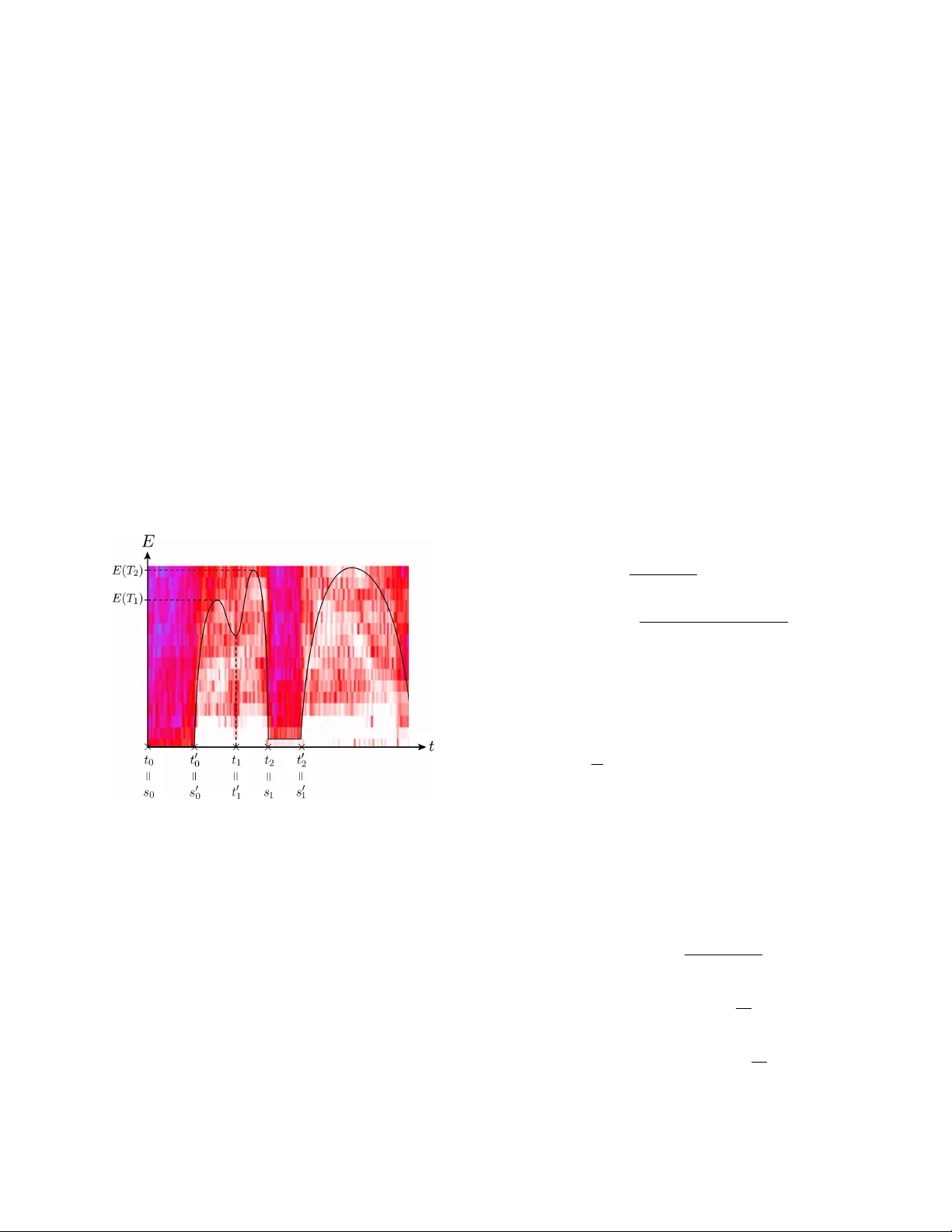
A UTOMA TIC CONFLICT DETECTION IN POLICE BOD Y -WORN A UDIO Alistair Letcher 1 , † J elena T ri ˇ sovi ´ c 2 , † Collin Cademartori 3 Xi Chen 4 J ason Xu 5 † Joint first authors 1 Uni versity of Oxford 2 Uni versity of Belgrade 3 Bro wn Uni versity 4 Carleton College 5 Uni versity of California, Los Angeles ABSTRA CT Automatic conflict detection has gro wn in relev ance with the advent of body-worn technology , but existing metrics such as turn-taking and ov erlap are poor indicators of conflict in police-public interactions. Moreov er , standard techniques to compute them fall short when applied to such di versified and noisy contexts. W e dev elop a pipeline catered to this task combining adapti ve noise removal, non-speech filtering and new measures of conflict based on the repetition and intensity of phrases in speech. W e demonstrate the effecti veness of our approach on body-worn audio data collected by the Los Angeles Police Department. Index T erms — Conflict detection, speech repetition, body-worn audio. 1. INTR ODUCTION Body-worn technology is be ginning to play a crucial role in providing evidence for the actions of police officers and the public [1], but the quantity of data generated is far too large for manual re view . In this paper we propose a nov el method for automatic conflict detection in police body-worn audio (BW A). Methodologies from statistics, signal processing and machine learning play a bur geoning role in criminology and predictiv e policing [2], but such tools have not yet been ex- plored for conflict detection in body-w orn recordings. More- ov er , we find that existing approaches are ineffecti ve when applied to these data off-the-shelf. Notable papers on conflict escalation inv estigate speech ov erlap (interruption) and con versational turn-taking as indi- cators of conflict in political debates . In [3], o verlap statistics directly present in a hand-labelled dataset are used to predict conflict, while [4] detect ov erlap through a Support V ector Machine (SVM) with acoustic and prosodic features. The work in [5] compares variations on both methods. Using au- tomatic overlap detection, their method achiev es 62 . 3% un- weighted conflict accuracy at best in political debate audio. This approach is all the less effecti ve on BW A data, which i s far noisier and more di verse. Besides being harder to detect, ov erlap serves as an unreliable proxy for conflicts between This research was supported by the LAPD and the UCLA Institute for Pure and Applied Mathematics, NSF Grant DMS-0931852. police and public: these often in volve little to no interruption, especially in scenarios where the of ficer is shouting or other - wise dominating the interaction. W e propose new metrics that successfully predict conflict in BW A along with speech processing and modeling tech- niques tailored to the characteristics of this data. Section 2 details adaptiv e pre-processing stages, feature extraction, and a SVM for non-speech discrimination. In Section 3, we dev elop metrics based on repetition using audio fingerprint- ing and auto-correlation techniques. This is based on the observation that conflict largely occurs in situations of non- compliance, where the offi cer repeats instructions loudly and clearly . Finally , performance is e v aluated on a dataset of 105 BW A files provided by the Los Angeles Police Department (LAPD) in Section 5. The illustration below summarizes our conflict detection procedure. Denoising Feature Extraction Non-Speech Filter Repetition Detection Conflict Score 2. PRE-PR OCESSING AND FIL TERING The success of our approach relies on pre-processing steps catered to the task at hand. W e apply adaptiv e denoising pro- cedures follo wed by feature extraction for supervised discrim- ination of non-speech, also called V oice Activity Detection. 2.1. Denoising Persistent noise like traffic, wind and babble as well as short- term bursts of noise including sirens, closing doors and po- lice radio are present along with speech in BW A audio. W e filter persistent but non-stationary background noise based on optimally-modified log-spectral amplitude (OM-LSA) speech estimation, and apply minima controlled recursi ve averaging (MCRA) as described in [6]. Briefly , this approach computes the spectral gain while accounting for speech presence un- certainty , ensuring that noise removal best preserves speech components ev en when the signal-to-noise ratio (SNR) is low . Let x ( n ) and d ( n ) denote speech and (uncorrelated, ad- ditiv e) noise signals respectively . Then the observed signal is y ( n ) = x ( n ) + d ( n ) , where n is a discrete-time index. The spectrum is obtained by windowing y ( n ) and applying the short-term Fourier transform (STFT), denoted Y ( k, l ) with frequency bin k and time frame l . The STFT of clean speech X ( k , l ) can be estimated as ˆ X ( k , l ) = G ( k , l ) Y ( k, l ) , where G ( k , l ) is the spectral gain function. V ia the LSA estimator , we apply the spectral gain function which minimizes E h ( log | X ( k , l ) | − log | ˆ X ( k , l ) | ) 2 i . Let hypotheses H 0 ( k , l ) and H 1 ( k , l ) respectively indicate speech absence and presence in the k th frequency bin of the l th frame. Assuming independent spectral components and STFT coefficients to be complex Gaussian variates, the spec- tral gain for the optimally modified LSA is gi ven by G ( k , l ) = G H 1 ( k , l ) p ( k,l ) G 1 − p ( k,l ) min . Here G H 1 ( k , l ) represents the spectral gain which should be applied in the case of speech presence and G min is the lower threshold for the gain in case of speech absence, preserving noise naturalness. p ( k , l ) is the a posteriori speech proba- bility P ( H 1 ( k , l ) | Y ( k, l )) , computed using the estimates of noise and speech variance λ d ( k , l ) and λ x ( k , l ) , the a priori SNR ξ ( k , l ) = λ x ( k,l ) λ d ( k,l ) and the a priori speech absence proba- bility q ( k , l ) = P ( H 0 ( k , l )) . T o estimate the time-varying spectrum of non-stationary noise λ d ( k , l ) , we employ temporal recursiv e smoothing dur- ing periods of speech absence using a time-varying smoothing parameter . The smoothing parameter depends on the estimate of the speech presence probability , obtained from its previ- ous v alues and the ratio between the local energy of the noisy signal and its derived minimum. Giv en ˆ λ d ( k , l ) we may im- mediately estimate the a posteriori SNR, γ ( k , l ) = | Y ( k , l ) | 2 λ d ( k , l ) . This is used to estimate the a priori SNR giv en by ˆ ξ ( k , l ) = αG H 1 ( k , l − 1) 2 γ ( k , l − 1) + (1 − α ) max { γ ( k , l ) − 1 , 0 } , with weight α controlling the noise reduction and signal dis- tortion. The estimate ˆ ξ ( k , l ) allows for computing the prob- ability of a priori speech absence as described in [6], which finally enables computation of the spectral gain and in turn speech spectrum. W e perform this filtering method three times in sequence to reliably remove residual noise that may persist after one stage of filtering. Doing so produces e xcellent results, elimi- nating most persistent noise while crucially a voiding attenua- tion of weak speech components. Nevertheless, sudden bursts of noise are rarely eliminated because the filter cannot adapt in time. W e apply the method belo w to remov e them, which is equally crucial to reliable repetition detection. 2.2. Featur e Extraction and Non-Speech Filter The task of this section is to filter remaining non-speech. T o begin, the audio signal is split into ov erlapping frames of size 0 . 06 s and with 0 . 02 s steps between start times. Ov er each frame, we compute 23 short-term features consisting of the first 13 Mel-Frequency Cepstral Coefficients (see [7]); zero- crossing rate; energy and energy entropy; spectral centroid, spread, entropy , flux and rolloff; fundamental frequency and harmonic ratio. Features which require taking the Discrete Fourier T ransform are first re-weighted by the Hamming win- dow . Since many meaningful speech characteristics occur in a longer time-scale, we additionally include the mid-term features obtained by averaging our short-term features across frames of size 0 . 3 s and step 0 . 1 s. W e apply a SVM with Radial Basis Function kernel [8, Chap. 12] to discriminate between speech and non-speech in this feature space. The SVM is trained on 38 minutes ( 22733 frames) of labeled speech and 47 minutes ( 28239 frames) of non-speech from BW A data. T o ev aluate predicti ve power we perform cross-validation (CV) with 10 folds [8, Chap. 7]. Our results are displayed in T able 1 and compare fav ourably with state-of-the-art papers in speech detection, which obtain error rates no lower than 5% in [9] and 12% in [10], on clean and noisy data (SNR at least 15 dB) respecti vely . Their learn- ing algorithms include SVMs, Gaussian Mixture Models and Neural Networks. False Positi ve False Ne gati ve T otal Error 1 . 26% 3 . 61% 2 . 31% T able 1 : 10 -fold CV error in speech/non-speech detection. 3. REPETITION DETECTION AND SCORING Having eliminated most of the non-speech and noise, we turn to detecting repetitions as a measure of conflict. W e split the audio into regions of interest and compare them using finger- print and correlation methods based on [11] and [12]. 3.1. Segmentation and Repetition In order to reduce the time it takes to search for repetitions, we automatically break the signal into regions which contain entire syllables, words, or phrases. W e begin by applying a band-pass filter between 300 and 3000 Hz, which we found to carry the most information about speech in our recordings. Let E 0 ( t ) be the energy (squared amplitude) of the sig- nal in a window of length 0 . 05 s starting at time t , and define E ( t ) = 1 { E 0 ( t ) > 0 . 05 } E 0 ( t ) . This threshold filters windows with energy below 0 . 05 , in which the signal-to-noise ratio is too small for reliable repetition detection. W e define points t 0 = 0 and t 1 , . . . , t n by the following criteria: 1. E ( t i ) is a local minimum of E ( t ) . 2. There exists t ∈ [ t i − 1 , t i ] such that E ( t ) 6 = E ( t i ) . 3. Each t i is the earliest time satisfying (1) and (2) . This somewhat cumbersome definition deals with the possi- bility that E attains the same local minimum value at con- secutiv e times, by taking the earliest such time. W e define t 0 1 , . . . , t 0 n analogously by taking the latest such times. This defines re gions [ t 0 i − 1 , t i ] delimited by local minima which are not trivially flat inside. W e then let T i be the earliest time in [ t 0 i − 1 , t i ] such that E ( T i ) is a local maximum. Finally , let s 0 = 0 and define ne w endpoints s j recursiv ely by s j = min { t i | t i ≥ s j − 1 and E ( T i ) − E ( t i ) > σ } , where σ is the standard de viation of E . W e define s 0 j analo- gously with t, s replaced by t 0 , s 0 ev erywhere. This isolates regions R j =  s 0 j − 1 , s j  which start at the bottom of an en- ergy spike and finish at the other end, ignoring spik es that are too small to be meaningful. The definitions are illustrated in Figure 1 belo w , where one of our BW A spectrograms is over - laid with a depiction of its energy curv e. Fig. 1 : Spectrogram o verlayed with ener gy across time. In this example, the local minimum t 1 = t 0 1 is not equal to any s j because the energy distance E ( T 1 ) − E ( t 1 ) to the previous maximum is less than σ . The resulting regions usually contain syllables or short words. In order to form regions of longer words and short phrases, we concatenate these initial regions together . First we choose a cutoff distance C = 0 . 02 s and let k = 0 . For each region R j = [ r 1 j , r 2 j ] , proceed as follows. If   r 2 j + k − r 1 j + k +1   < C then add a new region [ r 1 j , r 2 j + k +1 ] , increment k , and repeat until the condition is false. Finally , segments shorter than 0 . 05 s are discarded since any syllable takes longer to pro- nounce. These contain too little information to be reliably distinguished, and do not provide meaningful repetitions. Fingerprinting: Follo wing [11], our first measure associates a binary rectangular array called fingerprint to each region, and computes the percentage of entries at which two arrays differ . Regions are binned into N non-overlapping windows of length 0 . 1 s in the time domain, which are then partitioned into M = 32 bands of equal length between 300 and 3000 Hz in the frequency domain. W e define E n,m to be the energy of window n within frequenc y band m for 1 ≤ n ≤ N , 1 ≤ m ≤ M . W e then take second-order finite differences ∆ 2 ( n, m ) = [ E n,m − E n,m +1 ] − [ E n − 1 ,m − E n − 1 ,m +1 ] , which provide a discretized measure of curv ature in the spectral energy distribution over time. The value of the fin- gerprint at position ( n, m ) is no w defined as F ( n, m ) = 1 { ∆ 2 ( n,m ) > 0 } . Giv en a fingerprint pair , the percentage of positions at which arrays differ provides a measure E of dissimilarity between regions. Correlation: The second metric, based on [12], makes use of the correlation between Fourier coefficients over short win- dows. Regions R 1 and R 2 are first split into N overlapping windows w i 1 , . . . , w i N for i = 1 , 2 . For each window w i n , let ˆ w i n ( m ) be the Fourier coef ficients corresponding to frequen- cies between 300 and 3000 Hz. For each m , we compute the correlation C ( m ) = σ 1 , 2 ( m ) σ 1 ( m ) σ 2 ( m ) between the values of the m th coefficient of the tw o regions, where σ i ( m ) = v u u t N X n =1 ( ˆ w i n ( m ) − ˆ w i ( m )) 2 , σ 1 , 2 ( m ) = N X n =1 ( ˆ w 1 n ( m ) − ˆ w 1 ( m ))( ˆ w 2 n ( m ) − ˆ w 2 ( m )) , and ˆ w i ( m ) = 1 N P N n =1 ˆ w i n ( m ) . Finally , averaging C ( m ) ov er m = 1 , . . . , M yields an overall similarity measure C for R 1 and R 2 . This measure is less sensitiv e and produces more f alse positi ves than fingerprints. On the other hand, cor - relation can pick up on noisy repetitions where fingerprints fail. Our approach is to combine these methods so as to bal- ance their strengths and weaknesses. 3.2. Scoring Combining the fingerprint and correlation metrics into a sin- gle score, define S ( E , C ) = p f 1 ( E ) f 2 ( C ) where f 1 ( E ) = 1 { E < 0 . 3 } + 1 { 0 . 3 ≤ E ≤ 0 . 45 }  20 3 (0 . 3 − E ) + 1  , f 2 ( C ) = 1 { C > 0 . 55 } + 1 { 0 . 25 ≤ C ≤ 0 . 55 }  10 3 ( C − 0 . 25)  . The functions f 1 and f 2 are designed to conv ert the outputs of each method to more meaningful le vels of confidence that can be compared and combined, taking into account our empirical observations about the behavior of each method. For exam- ple, both our experiments and the paper [11] suggest that a fingerprint dif ference abov e 45% corresponds to regions that are almost certainly not repetitions. Similarly , we are almost certain that a fingerprint difference below 30% corresponds to repeated regions. After e v aluating segments, the measures are aggreg ated to score the entire audio file. This total score is computed as the av erage of non-zero scores among the top 5% of unique comparisons. As such, this score is higher for files that contain more or clearer repetitions, and lo wer for those with fewer or less distinguishable repetitions. Though repetition tends to be more frequent in scenarios of conflict, significant disputes can further be distinguished from mild ones via a measure of intensity . High conflict sce- narios often in volv e shouting or loud commands, producing higher energy . Accordingly , an intensity score is computed by averaging the energy among the same top 5% set of rep- etitions. The overall conflict score for an audio signal is the product of its repetition and intensity scores. 4. RESUL TS AND DISCUSSION W e test our approach on a collection of 105 body-worn audio files provided by the LAPD, of lengths between 3 and 30 min- utes each. The files are manually labeled according to level of conflict, where the classes and criteria are as follows: 2. High conflict (3 files): activ e resistance, escape, draw- ing of weapon, combativ e arguments. 1. Mild conflict (15 files): questioning of officer judg- ment, av oiding questions, av oiding to comply with commands, aggressiv e tone. 0. Low conflict (87 files): none of the abov e. Figure 2 is a plot of files ranked in descending order of con- flict score as determined by our method, illustrating that those labeled as high or mild conflict are concentrated toward the top. More specifically , all three files labeled as high conflict occur in the top 10 scores. In general, the three classes are correctly prioritized by the scoring algorithm. Only 4 of the 18 files in classes 1 and 2 fell below rank 24 . In other words, 78% of the files with any con- flict w ould be found by re viewing only the top 23% of files in the list. The mean scores for each class, displayed in the fig- ure, are clearly well-separated. Our method can thus be used to significantly reduce the time it takes to manually locate files containing conflict. Further , the algorithm automatically iso- lates the repetitions detected in a given file, which amount to very short audio portions relativ e to the entire signal. As such, we may quickly search through the high-rank audio files by listening to these portions. Giv en a larger dataset, one could automatically determine the adequate scores to label a file as containing high/mild/lo w 0 10 20 30 40 50 60 70 80 90 100 Rank 0 1 2 3 4 5 6 7 8 Score High Mild Low Fig. 2 : Plot of conflict score against rank. Horizontal lines depict the mean score for the class of corresponding color . conflict using a learning algorithm of choice. One may also input the fingerprinting, auto-correlation and intensity mea- sures as features into the learning algorithm, producing a de- cision hyperplane in three dimensions. In addition to their immediate use, our findings may also inform policy to better aid future work. W e find that officer speech is vastly more informativ e than other voices, which are less comprehensible and contribute to false positiv es. T o further improv e performance, one may exclude all speech except that of the officer . This falls under the task of speaker diarization—see [13] for a recent revie w—and most stud- ies in this area are based on relatively clean data (broadcast meetings, conference calls). State-of-the-art methods includ- ing [14] and [15] achieve no less than 18% diarization error rate on av erage, rising to 30% for some of the meetings, but perform much worse when applied to our BW A data. This obstacle may be overcome provided additional labeled data. Giv en a sample of the of ficer’ s voice that can be used to iden- tify them else where, our supervised learning task translates to speaker v erification [16]. Such data could be pro vided by requiring officers to record a few minutes of clean speech once in their career; this sample could then be ov erlaid with non-speech extracted by our pipeline to render it comparable with BW A files featuring a range of noise environments. 5. CONCLUSION T o summarize, we offer a novel method for automatic con- flict detection which is successful for applications in police body-worn audio. W e are able to automatically select audio files which are very likely to contain conflict, despite a small number of high conflict files. W e propose eliminating non- officer speech through speaker v erification and using all three sub-scores as learning features to improv e these results. 6. REFERENCES [1] Barak Ariel, W illiam A. Farrar , and Alex Sutherland, “The effect of police body-worn cameras on use of force and citizens’ complaints against the police: A random- ized controlled trial, ” Journal of Quantitative Criminol- ogy , v ol. 31, no. 3, pp. 509–535, Sep 2015. [2] George O. Mohler , Martin B. Short, Sean Malinowski, Mark Johnson, George E. Tita, Andrea L. Bertozzi, and P . Jeffrey Brantingham, “Randomized controlled field trials of predictiv e policing, ” Journal of the Ameri- can Statistical Association , v ol. 110, no. 512, pp. 1399– 1411, 2015. [3] F ´ elix Gr ` ezes, Justin Richards, and Andrew Rosen- berg, “Let me finish: automatic conflict detection using speaker ov erlap, ” in Interspeech , 2013. [4] Marie-Jos ´ e Caraty and Claude Montaci ´ e, Detecting Speech Interruptions for Automatic Conflict Detection , pp. 377–401, Springer International Publishing, 2015. [5] Samuel Kim, Sree Harsha Y ella, and Fabio V alente, “ Automatic detection of conflict escalation in spoken con versations, ” in Interspeech . ISCA, 2012. [6] Israel Cohen and Baruch Berdugo, “Speech enhance- ment for non-stationary noise en vironments, ” Signal Pr ocessing , vol. 81, no. 11, pp. 2403–2418, 2001. [7] Kishore Prahallad, “Speech technology: A practical introduction, topic: Spectrogram, cepstrum, and mel- frequency analysis, ” Carnegie Mellon Univ ersity , 2011. [8] Tre vor Hastie, Robert T ibshirani, and Jerome Friedman, The Elements of Statistical Learning , Springer-V erlag New Y ork, 2009. [9] Benjamin Elizalde and Gerald Friedland, “Lost in se g- mentation: Three approaches for speech/non-speech de- tection in consumer-produced videos, ” in Multimedia and Expo (ICME), 2013 IEEE International Conference on . IEEE, 2013, pp. 1–6. [10] Y uexian Zou, W eiqiao Zheng, W ei Shi, and Hong Liu, “Improv ed voice acti vity detection based on support vector machine with high separable speech feature vec- tors, ” in 2014 19th International Confer ence on Digital Signal Pr ocessing , Aug 2014, pp. 763–767. [11] Jaap Haitsma and T on Kalker , “ A highly robust audio fingerprinting system with an ef ficient search strategy , ” Journal of Ne w Music Resear ch , v ol. 32, no. 2, pp. 211– 221, 2003. [12] Cormac Herley , “ ARGOS: Automatically extracting repeating objects from multimedia streams, ” T rans. Multi. , vol. 8, no. 1, pp. 115–129, Sept. 2006. [13] Xavier Anguera, Simon Bozonnet, Nicholas Evans, Corinne Fredouille, Gerald Friedland, and Oriol V inyals, “Speaker diarization: A revie w of recent re- search, ” IEEE T ransactions on Audio, Speech, and Lan- guage Pr ocessing , vol. 20, no. 2, pp. 356–370, 2012. [14] Gerald Friedland, Adam Janin, David Imseng, Xavier Anguera, Luke Gottlieb, Marijn Huijbregts, Mary T ai Knox, and Oriol V in yals, “The ICSI R T-09 speaker di- arization system, ” IEEE T ransactions on Audio, Speec h, and Language Processing , v ol. 20, no. 2, pp. 371–381, 2012. [15] Emily B. Fox, Erik B. Sudderth, Michael I. Jordan, and Alan S. Willsk y , “ A stick y HDP-HMM with application to speaker diarization, ” The Annals of Applied Statistics , vol. 5, no. 2A, pp. 1020–1056, 06 2011. [16] Douglas A. Reynolds, Thomas F . Quatieri, and Robert B. Dunn, “Speaker verification using adapted Gaussian mixture models, ” Digital signal pr ocessing , vol. 10, no. 1-3, pp. 19–41, 2000.