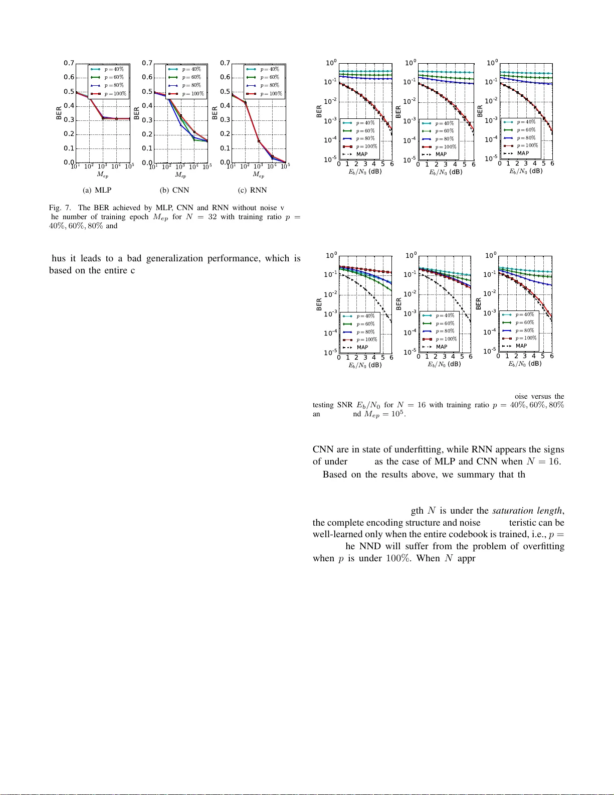
Performance Evaluation of Channel Decoding With Deep Neural Networks

Performance Ev aluation of Channel Decoding W ith Deep Neural Networks W ei L yu, Zhaoyang Zha ng † , Chunx u Jiao, Kan gjian Qin, and Hu azi Zha n g College of Inf ormation Science an d Electronic Eng ineering, Zhejiang Un i versity , Hangzhou, China. Provincial Ke y Lab o f Info . Proc., Commu n. & Netw . (IPCAN), Zhejiang , Chin a . E-mails: † ning ming@zju.ed u.cn Abstract —With the demand of high data rate and low latency in fifth generation (5G), deep neural n etwork decoder (NND) has become a promising candidate due to its ca pability of one-shot decoding and parallel computin g. In this paper , three types of NN D, i.e., multi-layer perceptron (MLP), con volution neural netwo rk (CNN) and recurr en t neural network (RNN), are proposed with the same parameter magnitud e. Th e performance of these deep neu ral networks are ev aluated through extensive simulation. Numerical results sho w that RNN has the best decod- ing performa nce, yet at the price of the highest computational ov erhead. Moreov er , we find there exists a saturation length for each type of neural n etwork, which is caused by their restr icted learning abilities. I . I N T RO D U C T I O N Recently , the long- term evolution, also known as fifth gen- eration (5G), h as been widely rolled out in many co untries. There is no do ubt that 5G can accommodate the rapid in- crease o f u ser data and system capacity . In tuitiv e ly , hig her transmission rate requires lower decoding laten cy . Howev er , conv e n tional decod ing algorithm s suffer from high decoding complexity th at inv o lves a nu mber o f iterativ e calcu lations. As su ch, d esigning n ew high-speed low-latency deco ders has become an emerging issue to be cop ed with. Recent a dvances in deep learning provide a n ew direction to tackle th is pro b lem. Deep lear n ing [1] has be en applied in computer v ision [2], n atural language pro cessing [ 3], au- tonomo us vehicles [4] and many other areas. The remark- able results verify its g ood p erform ance. Inspire d by this, the gene r al d ecoding prob lem ca n be viewed as a form of classification, which is a typica l application of deep learn ing. In brief, the deep n eural ne twork u ses a cascad e o f multiple layers with non linear proc e ssing units to extract and transform features co ntained in encodin g structure and noise c harac- teristic. Com pared with c o n ven tio nal iterati ve decod ing, the deep neural network d ecoder (NND) calculates its estimator by passing ea c h lay er o n ly o nce with the pre-trained neural network, which is refer red to as one-sh ot dec oding. It provides a fo undation f or low-latency implem e ntations. In a d dition, the hig h -speed demand can be easily satisfied by utilizing the cu rrent d eep lea r ning p latforms, such as T ensorflow [5]. Generally , they support par allel computing and explo it the powerful hardwares like graph ical processing units (GPUs). Researchers have tried to solve ch annel deco d ing problem using deep neural network. The authors in [6] h av e dem on- strated that by assigning p roper weights to the p assing m es- sages in the T a nner graph , comparable decoding performance can be ach ieved with less iterations than tra d itional belief propag ation (BP) deco ders. These weigh ts are obtain ed via training in deep lea rning, which partially co mpensates for the effect of small cycles in the T anner gr aph. Conside r ing th at BP decodin g contains many multip lica tions, [7] pro posed a lig h t- weight neural offset min-sum decoding algorithm, with no multiplication and simple hardware im p lementation . [ 8] found that the stru ctured codes are indeed easier to lea r n than ran dom codes, an d addr e ssed the challenge that deep learning b ased decoder s are difficult to train fo r long codes. Conseq u ently , [9] propo sed to divide the p olar coding graph into sub-b locks, with the deco d er for each sub-codeword being trained separ ately . Although th e co mbination o f c h annel d ecoding an d deep neural network has been studied in the above w o rks, two im- portant pr oblems have not been fully in vestigated . First, wh ich type of deep n eural network is more su itab le for NND. Seco nd, how the length of codeword affects the NND p erform ance. In this paper, thre e typ es of NND, which build upon multi-layer perceptro n (MLP), conv olution neural n etwork (CNN) a nd recurren t neural network (RNN), are pro p osed with th e same parameter magnitude. W e com pare the perfo rmance amon g these three dee p neu ral n etworks thro ugh num erical simu la- tion, and find that the RNN has the best decod in g perfo rmance at the p rice of the highest com p utational overhead . Also, we find the leng th of codeword influences the fitting of d eep neural network (overfitting an d underfitting ). It is infe r red that there exists a saturation length for each type of dee p neur al network, which is caused by their r estricted learning a b ilities. The rest of th is paper is organized as fo llows. In Sectio n II, the system fr a m ew o r k an d the pro posed structu r es o f NND ar e provided. Section III shows th e nume rical results a n d pr ovides the co mparisons am o ng MLP , CNN and RNN that are trained with and w ith out no ise. Section IV conclude s this paper . I I . S Y S T E M D E S I G N In ord er to better p resent the design of NND, we fir st describe the system framework of NND. Spec ifically , the training process of NND is introduced in detail and the reason why we set some param eters like tr aining r atio o f co deboo k set is explain e d. Finally , we de scr ibe the pro posed stru ctures of MLP , CNN and RNN, respectively . Encoder BPSK Modulator Channel Deep Neural Network Decoder x u s y ˆ x Fig. 1. The archit ecture of deep neural networ k decoder . A. System F ramework The arc hitecture of NND is illustrated in Fig. 1. At the transmitter, we assume that the length of infor m ation bits x is K . T hen, x is encoded to a bina ry cod ew or d u of length N throug h a chan nel encode r , and th e cod eword u is then ma pped to a symbol vector s through the binary ph ase shift keying (BPSK) mod ulation. It is assumed that the BPS K symbols are transmitted in the ad ditiv e white Gaussian noise (A WGN) in this pap er . At the receiver , vector y is rece i ved and can be written as y = s + n , (1) where n ∼ N ( 0 , σ 2 I N ) repr esents the N × 1 symbol vector . The estimated informatio n bits ˆ x is decoded from y with the aid of the NND , where th e structur e of NND substantially affects the perfo rmance. For the no ta tio nal convenience of the following pap er , we denote that ˆ x , [ ˆ x 0 , . . . , ˆ x K − 1 ] , x , [ x 0 , . . . , x K − 1 ] , y , [ y 0 , . . . , y N − 1 ] , and we refer to the set of all possible x an d ˆ x as X and tha t o f all possible y as Y . Generally , the aim of decod ing algorithm is to find a optim a l map function f ∗ : Y → X , which satisfies the maximum a posteriori (MAP) criterion f ∗ ( y ) = ar g max x ∈X P ( x | y ) . (2) Obviously , we hope that th e NND ca n reach the p e rfor- mance of MAP decod ing as far as possible. As a super vised learning metho d , the construction of n eural network needs two phases, they are training phase an d testing phase, respe cti vely . During the trainin g p hase, a nu mber of training samples a r e used to correct the weigh ts and biases in the neu ral network with the aim of min imizing the lo ss function , and the map function f will be obtained after this phase. Then, the testing phase, whic h is th e actu a l deco ding phase, is just to estimate informa tio n bits from the ne w received symbol vector by f , and it is wh y we call it one -shot d ecoding . B. T raining T o design the training phase of neur al network, which greatly influen ces the decoding perfor mance of NND, we need solve two pr oblems. First, how to gener a te tra in ing samp les. Second, which type of loss fu nction should b e chosen. 1) Generating training samples: T o train the network, we need bo th r eceiv ed vector y and tru e informatio n bits x . As such, the gen eral sample generating proc e ss can be described like this: The inf ormation bits x is rand omly picked fr om X , and then the received vector y can be ob tained b y performing channel encodin g , BPSK mapping and simulated c h annel noise. · · · · · · · · · · · · · · · · · · 0 y 1 y 2 y 3 N y - 2 N y - 1 N y - Input Hidden Layer-1 Hidden Layer-2 Hidden Layer-3 Sigmoid Layer 64 Nodes 32 Nodes 16 Nodes Sigmoid 0 ˆ x 1 ˆ x 2 ˆ K x - 1 ˆ K x - · · · Output Fig. 2. The proposed archit ecture of multi-laye r percept ron. Howe ver, there are two impo rtant factors we have to con - sider in the design . One is the ratio of cod ebook set X du r ing training p hase, we denote it as p . If we just rand omly pick x from en tire set X in the tr aining p hase, th e new cod ew o rds received at testing phase may have been seen dur in g the training pha se, thus the p r ocess of neural network is m ore like recordin g an d reading , oth er than learnin g. T o ev alua te the g eneralization ab ility of N ND which means if the NND is able to estimate the unseen codewords, we set that th e informa tio n bits x is rando mly picked fro m X p which covers only p % o f th e entire set X . The o ther factor is the signal to noise ratio (SNR) of training samples, we denote it as ρ t . As the SNR of the actu al decoding pha se is u n known and time- varying, the p erforma nce of NND greatly de p ends o n the SNR of training samples. As in [8], we adopt the pro posed meth od for the settin g of train ing SNR and define a n ew performance metric which is called th e norma lize d validation erro r (NVE) as follows NVE ( ρ t ) = 1 S S X s =1 BER NND ( ρ t , ρ v, s ) BER MAP ( ρ v, s ) , (3) where ρ v, s denotes th e s -th SNR in a set of S different validation samples, BER NND ( ρ t , ρ v, s ) is the bit erro r rate (BER) achie ved b y a NND train ed at ρ t on the data with ρ v, s and BER MAP ( ρ v, s ) repr esents the BER o f MAP dec o ding at ρ v, s . As such, the NVE measures how g ood a NND, trained at a particular SNR, is compared to MAP decodin g over a range of dif fe r ent SNRs, an d it can be inferred that the less NVE indicates the better perform ance the NND. As [8] say s, there is always an optimal ρ t , wh ich can be explained b y the two extreme cases: • ρ t → + ∞ : train without noise, the NND is n ot tr a ined to hand le noise. • ρ t → −∞ : train only with noise, the NN can n ot learn the enco d ing structure. This clearly ind icates an optim um somewhere in between these two cases. For this reason, we tr ain the NND with datasets of · · · · · · · · · · · · · · · Input Convolution Layer Pooling Layer Output N x 1 vector Feature Maps Feature Maps K x 1 vector Fig. 3. The proposed archit ecture of con volutio n neura l net work. different ρ t in o ur work, and choo se the optimal ρ t which results in the least NVE. 2) Cost function: Loss fun ction is to mea sure the difference between the actual NND output and its expected outp ut, if the actual outpu t is close to the expected o utput, the loss sho uld be incremen ted only sligh tly whereas large erro rs should result in a very large loss. In o ur work, w e emp loy th e mean squared error (MSE) as th e loss fun ction, which is defined as L MSE = 1 K K − 1 X i =0 ( x i − ˆ x i ) 2 , (4) where x i ∈ { 0 , 1 } is the i -th target infor mation bit and ˆ x i is the i -th NND estimator . No tably , we make ˆ x i ∈ [0 , 1] by incurrin g a sigmoid functio n at the end o f NND, and it can be interp reted as the prob ability that a “1” was transmitted. Although there are other common ly used cost f unctions in neural network, our focus is to co mpare the NND per forman ce with dif f e rent types of deep neural network, a nd th e in fluence of cost function for each ty pe of NND is identical, thus w e just c hoose the MSE which is simple a nd ea sy understand ing. T ABLE I S U M M A RY O F T OTA L PA R A M E T E R N U M B E R Number of N MLP CNN RNN N = 8 3136 2072 2052 N = 16 3712 2456 3076 N = 32 4864 3992 5124 C. Design of Deep Neural Network In this sectio n , ou r sp ecific design s for MLP , CNN an d RNN are described. It is well k n own that if the p arameters of n eural network (weights and biases) are very large, the expression and learning ability of neural network usually will be very stro ng. Considering that o ur aim is to compa r e the learning ability of different d eep neural networks, we should keep the total parameter n u mber of each neura l n etwork app roximately the same, to a void that the perfor mance difference o f deep n eural networks comes f rom the d ifference of parameter number . As such, we construct a relative simple and gen eral structur e for T ABLE II PA R A M E T E R S O F C N N T ype of layer Kernel size / stride (or Annotation) Input size Con voluti on 3 × 1 / 1 N × 1 × 1 Pooling 2 × 1 / 2 N × 1 × 8 Con voluti on 3 × 1 / 1 N/ 2 × 1 × 8 Pooling 2 × 1 / 2 N/ 2 × 1 × 16 Con voluti on 3 × 1 / 1 N/ 4 × 1 × 16 Pooling 2 × 1 / 2 N/ 4 × 1 × 32 Con voluti on N/ 8 × 1 / 1 N/ 8 × 1 × 32 Squeeze Reduce the dimension 1 × 1 × K Sigmoid Output the classificati on probabilit y 1 × K each neural network, an d keep the m a gnitude of param e te r s as 10 3 , whic h is sh own in T a b le I . MLP is a class of feed forward a rtificial neur al network with fully connection between layers, which consists of at least three layers of node s. Each n ode o f MLP is a neuron that uses a no n linear activ atio n function wh ich gives it lea r ning ability . It is shown in [10] that nonlinear acti vation functions can theo retically appr o ximate any continu ous functio n on a bound ed region arbitrar ily closely if the number of neuro n s is large enoug h. In this paper, the propo sed architecture o f MLP is described in Fig. 2. W e em p loy three hidd en layer s with 64, 32, 16 in MLP , and the nodes of input layer and output layer is N and K with n o dou b t. CNN is a lso a class of f eedforward artificial neur al net- works which has been successfully applied to analyzing visual imagery . The hidden layer s of CNN are either conv olutional or po o ling, wh ich emulate d th e respo nse of an in dividual neuron to v isual stimuli [11], and the conv olu tion operatio n significantly r educes th e nu mber of parameter s, allowing the network to be deeper with fewer para meters. As such, the excellent perfo rmance of CNN fo r the image cha r acteristic extraction moti vates us to comb in e CNN with NND in this work. Considering that CNN is usually used fo r image, some modification s ar e neede d when apply ing CNN in NND. As Fig. 3 shows, we mo dify the each layer’ s input o f CNN a s a 1-D vector instead of a 2 -D im age. Also, we employ a general structure of CNN witho ut some high -lev el tricks like b atch normalizatio n pre sen ted in [ 1 3], the detailed para meter setting is listed in T able II. RNN is a class of artificial n eural ne twork wh ere con nec- tions between units f orm a directed cycle. This allows it to exhibit dynam ic temporal b ehavior . Unlike feedforward neura l networks, RNN can use their internal memory to pro cess arbitrary sequences of inpu ts. Th is makes them ap plicable to tasks such as unsegmented , connected han d writing recog ni- tion or sp e e ch reco gnition [12]. Inspire d by the remark able perfor mance of RNN on the time series task, we ho pe it can also ach ie ve a good per f ormance in NND. No ta b ly , general RNN suffers a ser io us vanishing gradient pr oblem as described in [15], p eople usually adop t long short-ter m memory (LSTM) in practice. As pre sented in [14], LSTM contains thr ee gates, called forget gate, in put gate and o utput gate respectively , to con tr ol th e inform ation flow , which can s s tanh s tanh Input Gate Output Gate Forget Gate t y t -1 c t -1 h t c t h (a) Basic L S T M cell 0 c LSTM Cell LSTM Cell LSTM Cell Sigmoid 0 ˆ x 1 ˆ K x - · · · · · · 0 y 1 y 1 N y - · · · · · · · · · 0 h 1 c 1 h 1 , 255 N h - 1 , 0 N h - (b) The flow diagram of LSTM. Fig. 4. T he proposed archite cture of long s hort-te rm memory (LSTM). prevent bac k propa g ated erro rs from vanishing or explod ing. As such , we take LSTM as the represen tati ve of RNN, and the propo sed arch itec tu re is described in Fig. 4. W e set the outpu t dimension of LSTM cell is 256, i.e., h and c are 256 × 1 vectors, an d only o ne LSTM cell is emp loyed in each time step. T ABLE III H Y P E R PA R A ME TE R S E T T I N G Size of training samples 10 6 Size of testing samples 10 5 Mini-bat ch size 128 Dropout probabi lity 0 . 1 Initia lizat ion method Xavi er initi alization Optimiza tion method Ada m opt imization I I I . P E R F O R M A N C E E V A L UAT I O N In this section , the per formanc es of NND with MLP , CNN and RNN f or different len gth of N are c ompared . Thro ugho u t all exper iments, we use a p olar code of rate 1 / 2 and set the codeword length N as 8 , 16 , 32 . The training ratio of codebo ok p is set as 40 % , 60% , 80% and 100% . W e take 12 different SNR points from − 2 d B to 2 0 dB as tra in ing SNR ρ t , an d as mention ed b efore, the best ρ t , wh ich results in the least NVE, will be chosen for testing phase. For the setting o f g eneral par ameters in neural network, which are called hyper parameter s [16], we cho ose a relativ ely reason able and satisfyin g set as sho wn in T ab le II I after a lo t of trials. Notably , we use T ensorflow as our experimen ta l platform , a n d the sou rce code 1 is available for repr oducible research. T o b etter ev alu ate the learn ing ability of NND, we divide the simulation into two parts. First part inv estigates the per - forman ce of NND that are trained without noise, w h ich only 1 https:/ /github .com/le vylv/deep-neural-network-decoder 10 1 10 2 10 3 10 4 10 5 M e p 0 . 0 0 . 1 0 . 2 0 . 3 0 . 4 0 . 5 0 . 6 0 . 7 BE R p = 40% p = 60% p = 80% p = 100% (a) MLP 10 1 10 2 10 3 10 4 10 5 M e p 0 . 0 0 . 1 0 . 2 0 . 3 0 . 4 0 . 5 0 . 6 0 . 7 BE R p = 40% p = 60% p = 80% p = 100% (b) CNN 10 1 10 2 10 3 10 4 10 5 M e p 0 . 0 0 . 1 0 . 2 0 . 3 0 . 4 0 . 5 0 . 6 0 . 7 BE R p = 40% p = 60% p = 80% p = 100% (c) RNN Fig. 5. The BER achie ved by MLP , CNN and RNN without noise ver- sus the number of trainin g epoch M ep for N = 8 with trai ning ratio p = 40% , 60% , 80 % an d 100% . 10 1 10 2 10 3 10 4 10 5 M e p 0 . 0 0 . 1 0 . 2 0 . 3 0 . 4 0 . 5 0 . 6 0 . 7 BE R p = 40% p = 60% p = 80% p = 100% (a) MLP 10 1 10 2 10 3 10 4 10 5 M e p 0 . 0 0 . 1 0 . 2 0 . 3 0 . 4 0 . 5 0 . 6 0 . 7 BE R p = 40% p = 60% p = 80% p = 100% (b) CNN 10 1 10 2 10 3 10 4 10 5 M e p 0 . 0 0 . 1 0 . 2 0 . 3 0 . 4 0 . 5 0 . 6 0 . 7 BE R p = 40% p = 60% p = 80% p = 100% (c) RNN Fig. 6. The BER achi e ved by MLP , CNN and RNN without noise versus the number of traini ng epoch M ep for N = 16 with training ratio p = 40% , 60% , 80% and 100% . reflects the learning ability for enco ding structure. Seco n d part in vestigates the perf ormance of NND that are trained with noise, which in volves the sim u ltaneous learnin g f or en coding structure and noise char acteristic. Addition ally , the system perfor mance is measured by th e bit error rate (BER) based o n the testing samples, and the per forman c e of MAP decod ing is compare d as a bench mark. A. Learning without Noise Fig. 5 invest igates the BER achieved b y MLP , CNN and RNN w ith out noise as a function of the numbe r of training epochs ranging from M ep = 10 1 , . . . , 10 5 for N = 8 , with respect to different training ratio of cod e b ook. From Fig. 5, we can see that the BER d ecreases gradually with the number of training epoch in creasing, and it fina lly reaches a steady value, which rep r esents th e conv e rgence of deep neural network. For all three deep neu ral networks, it can be ob served that th e lower p leads to highe r BER, and only when p = 100% the BER dro ps to 0 , wh ich deno tes the n eural network s have learned the complete encoding structure. The pheno m enon can b e explained as the overfitting of n eural network , i.e., the n eural network can fit the relationship be tween in put and output very well fo r each value o f p e ven if it is not 100% , 10 1 10 2 10 3 10 4 10 5 M e p 0 . 0 0 . 1 0 . 2 0 . 3 0 . 4 0 . 5 0 . 6 0 . 7 BE R p = 40% p = 60% p = 80% p = 100% (a) MLP 10 1 10 2 10 3 10 4 10 5 M e p 0 . 0 0 . 1 0 . 2 0 . 3 0 . 4 0 . 5 0 . 6 0 . 7 BE R p = 40% p = 60% p = 80% p = 100% (b) CNN 10 1 10 2 10 3 10 4 10 5 M e p 0 . 0 0 . 1 0 . 2 0 . 3 0 . 4 0 . 5 0 . 6 0 . 7 BE R p = 40% p = 60% p = 80% p = 100% (c) RNN Fig. 7. The BER achi e ved by MLP , CNN and RNN without noise versus the number of traini ng epoch M ep for N = 32 with training ratio p = 40% , 60% , 80% and 100% . thus it leads to a bad g eneralization p e rforman ce, wh ich is based on the en tire codeb ook. The similar case but when N = 1 6 is studied in Fig. 6. For MLP , we fin d that wh en p = 1 00% , th e perfor mance is getting worse co m pared with the case of N = 8 , the reason is the size of co deboo k expo n entially increase with the growth of N , thus it induces a mor e comp lex relationship between the input and output of NND, wh ich goes beyond the lear n ing ability of current ne u ral network and make it tend to b e und erfitting. Howe ver, it is satisfied to see that when p = 60% and 80% , the BER drops to 0 , which r e presents the MLP is able to generalize fro m a fr action of c o deboo k to the entire c odeboo k set. The only difference o f CNN when compar ed with ML P is that when BER d rops to 0 , the p is 80% an d 100% , it ind icates the learning ability o f CNN is a little b it stron ger than ML P . Notably , the RNN is still in the state of overfitting since its perfor mance remains the same as th e case wh en N = 8 . Similarly , Fig. 7 is f or th e case when N = 32 . Obviously , it can be inferred th at both of MLP and CNN are in state of u nderfitting. Howe ver , RNN can achieve a very good perfor mance bec a use the BER drop s to 0 with each value of p , it proves that RNN is better th an MLP and CNN fo r NND. B. Learning with Noise In this p art, we r esearch the case with n o ise which inv olves the simultaneous learning for en coding structure and noise characteristic, and th e BER perf ormances versus the testing SNR E b / N 0 for d ifferent codeword le n gth N are inves tigated. Fig. 8 studies the case when N = 8 , it ca n be observed that MLP , CNN and RNN can all achieve MAP performa nce whe n p = 100% , althoug h they are overfitting wh en p is under the 100% . Similarly , Fig. 9 stud ies the case when N = 16 . For both MLP and CNN, we find that the four curves of different training ratio p are very close an d have a certa in gap co mpared with MAP curve, it indicated that b oth of MLP an d CNN tend to be underfitting , alth o ugh CNN is a little better th an MLP . Howe ver, RNN still keeps overfitting who can ach iev e MAP perfor mance when p = 100% . From Fig. 10, wh ich studies the case wh en N = 32 , we can con clude that both of ML P and 0 1 2 3 4 5 6 E b /N 0 ( d B) 1 0 - 5 1 0 - 4 1 0 - 3 1 0 - 2 1 0 - 1 1 0 0 BE R p = 40% p = 60% p = 80% p = 100% M AP (a) MLP 0 1 2 3 4 5 6 E b /N 0 ( d B) 1 0 - 5 1 0 - 4 1 0 - 3 1 0 - 2 1 0 - 1 1 0 0 BE R p = 40% p = 60% p = 80% p = 100% M AP (b) CNN 0 1 2 3 4 5 6 E b /N 0 ( d B) 1 0 - 5 1 0 - 4 1 0 - 3 1 0 - 2 1 0 - 1 1 0 0 BE R p = 40% p = 60% p = 80% p = 100% M AP (c) RNN Fig. 8. The BER ac hiev ed by MLP , CNN and RNN with noise versus the testing SNR E b / N 0 for N = 8 with training ratio p = 40% , 60% , 80 % and 100% and M ep = 10 5 . 0 1 2 3 4 5 6 E b /N 0 ( d B) 1 0 - 5 1 0 - 4 1 0 - 3 1 0 - 2 1 0 - 1 1 0 0 BE R p = 40% p = 60% p = 80% p = 100% M AP (a) MLP 0 1 2 3 4 5 6 E b /N 0 ( d B) 1 0 - 5 1 0 - 4 1 0 - 3 1 0 - 2 1 0 - 1 1 0 0 BE R p = 40% p = 60% p = 80% p = 100% M A P (b) CNN 0 1 2 3 4 5 6 E b /N 0 ( d B) 1 0 - 5 1 0 - 4 1 0 - 3 1 0 - 2 1 0 - 1 1 0 0 BE R p = 40% p = 60% p = 80% p = 100% M A P (c) RNN Fig. 9. The BER ac hiev ed by MLP , CNN and RNN with noise versus the testing SNR E b / N 0 for N = 16 with trai ning ratio p = 40% , 60% , 80% and 100% and M ep = 10 5 . CNN are in state of under fitting, while RNN appears th e sign s of un d erfitting as the case of MLP and CNN when N = 16 . Based on th e results above, we summary that there e xists a saturation length for each typ e of deep neura l network in NND, w h ich is caused by their restricted learning a bilities. When th e codeword length N is un der the saturation length , the comple te e n coding structure an d noise char a cteristic can be well-learned only when the entire co debook is trained, i.e. , p = 100% , the NND will suffer from the problem of overfitting when p is u n der 100% . When N ap proache s the satur ation length , the per f ormance s with different training ratio p are very close, and the NND tends to be und erfitting with the tra ining ratio p increasing. When N exceeds the sa turation length , th e NND is th oroug hly un d erfitting no matter wh at the p is. For the pro posed neural network architectu res in this paper, we can conclud e that the saturation leng ths of MLP and CNN are both 16 d e sp ite that the learn ing ability of CNN is a little stronger th an MLP , while the satu ration length of RNN is 32 . W e fu r ther inv estigate the co mputation al time o f MLP , CNN and RNN as shown in Fig . 11. As mention ed before, we keep the same parameter m a g nitude for each neur al network, howe ver, the actual comp utational time is still very d ifferent due to their own specific structures. F o r both training and 0 1 2 3 4 5 6 E b /N 0 ( d B) 1 0 - 6 1 0 - 5 1 0 - 4 1 0 - 3 1 0 - 2 1 0 - 1 1 0 0 BE R p = 40% p = 60% p = 80% p = 100% M A P (a) MLP 0 1 2 3 4 5 6 E b /N 0 ( d B) 1 0 -6 1 0 -5 1 0 -4 1 0 -3 1 0 -2 1 0 -1 1 0 0 BE R p = 40% p = 60% p = 80% p = 100% M AP (b) CNN 0 1 2 3 4 5 6 E b /N 0 ( d B) 1 0 - 6 1 0 - 5 1 0 - 4 1 0 - 3 1 0 - 2 1 0 - 1 1 0 0 BE R p = 40% p = 60% p = 80% p = 100% M AP (c) RNN Fig. 10. T he BER achie ved by MLP , CNN and RNN with noise v ersus the testing SNR E b / N 0 for N = 32 with trai ning ratio p = 40% , 60% , 80% and 100% and M ep = 10 5 . N = 8 N = 1 6 N = 3 2 0 1 2 3 4 5 6 7 8 C o m p u ta ti o n a l t i m e ( s) 1 e − 4 M L P C N N R N N (a) N = 8 N = 1 6 N = 3 2 0 . 0 0 . 5 1 . 0 1 . 5 2 . 0 2 . 5 C o m p u ta ti o n a l t i m e ( s) 1 e − 4 M L P C N N R N N (b) Fig. 11. The computatio nal time of MLP , CNN and RNN versus the lengt h of code word N . (a) The backward propaga tion time for one training sample. (b) The forward propagat ion time for one testin g sample. testing phase, the comp utational time of RNN is muc h higher than that of MLP and CNN, while the compu tational time of CNN is just a little b it higher than that of ML P . As such, we can con clude that the perform ances of CNN an d MLP are very close, altho ugh CNN has b etter decodin g perfor mance but higher computa tio nal time in a small degree, and RNN can achie ve the best decodin g perfo rmance at the price of th e highest com putationa l time. I V . C O N C L U S I O N In this paper, we propo se three types of NND, which b uild upon MLP , CNN and RNN. W e com pare the performanc e among these three d eep n eural ne twork s thro ugh experimen t, and find that RNN has the best d ecoding per forman ce at the p rice o f the highest com putational time, and CNN has better deco ding perform ance but high er comp utational tim e than MLP in a small degree. W e find that th e length of codeword influences the fitting of deep neural network, i.e., overfitting and underfitting. It is inferr ed that there exists a saturation len gth for each type of neural network, wh ich is caused by their restricted learn ing abilities. Rem inding that the p r oposed structur es of ML P , CNN and RNN are relatively simple an d general, the focus o f our fu ture work is to design more co mplex structur e s to improve their sa turation lengths for the deman d of long er codew ords, for example, increasing neuron no des fo r MLP , adding co nvolution layers for CNN or stacking more LSTM cells in each time step. In the m eanwhile, the deco ding per f ormance with th e satu ration length must approx imate the MAP perf ormance as far as po ssible. A C K N O W L E D G E M E N T This work was supported in part by Natio nal Natural Science F ounda tion of China (Nos. 617 25104 , 61631 003), Huawei T echnolo gies Co.,Ltd (HF20 1 7010 0 03, YB20150 4 0053 , YB20 13120 029), and Educ a tion Foundation of Zhejian g Univ ersity . R E F E R E N C E S [1] Y . LeCun, Y . Bengio, and G. Hinton, “Deep learning, ” Nat ure , vol. 521, no. 7553, pp. 436, 2015. [2] K. He, X. Zhang, S. Ren, and J. Sun, “Deep residual learning for image recogni tion, ” in Pr oceedings of the IEEE Confer ence on Computer V ision and P atte r n Reco gnition , pp. 770–778, 2016. [3] I. Sutske ver , O. V in yals, and Q. V . Le, “Sequen ce to sequence le arning with neural netw orks, ” in Advances in Neural Information P r ocessing Systems (NIPS) , pp. 3104–3112, 2014. [4] C. Che n, A. Sef f, A. Kornh auser , and J. Xiao, “Deep dri ving: learning af fordance for direct perception in autono mous driving, ” in Pr oceedings of the IEE E Internati onal Confer ence on Computer V ision , pp. 2722–2730, 2015. [5] M. Abadi, P . Barham, and et al., “T ensor flo w: A system for large -s cale machine learning, ” in Proce edings of the 12th USENIX Symposium on Operat ing Systems Design and Implementati on (OSDI) , 2016. [6] E. Nachmani, Y . Beery , and D. Burshtein, “Learning to decode linear codes using deep learning, ” in The 54th Annual Allerton Confer ence on Communicat ion, Contr ol, and Computing , pp. 341–346, 2016. [7] L. Lugosc h and W . J. Gross, “Neural offset min-sum de coding, ” arXiv preprint , 2017. [Online]. A v ailable: http://arxi v .org/ab s/1701.05931 [8] T . Gruber , S. Cammerer , J. Hoydis, and S. ten Brink, “On deep learning- based channel decoding, ” in The 51st Annual Confere nce on Information Scienc es and Systems (CISS). IEEE , pp. 1–6, 2017. [9] S. Cammerer , T . Gruber , J. Hoydis, and S. te n Brink, “Scaling de ep learni ng-based decoding of polar codes via partiti oning, ” arXiv preprin t, 2017. [Online]. A va ilable: htt p://ar xi v . org/a bs/1702.06901 [10] K. Hornik, M. Stinchco mbe, and H. White, “Multilayer feedforward netw orks are univ ersal approximator s, ” Neural Net works , vol. 2, no. 5, pp. 359–366, 1989. [11] Y . LeCun, L . Bottou, Y . Bengi o, and P . Haffner , “Gradient -based learning applie d to docu ment recogn ition. ” Proc eedings of the IEE E vol . 86 no. 11, pp. 2278–2324, 1998. [12] S. Shelk e and S. Apte, “ A nov el multi-fea ture multi-cla ssifier scheme for unconstra ined handwritte n dev anagari charact er recogniti on, ” 2010 12th Internati onal Confere nce on F ronti ers in H andwriti ng Recogniti on , 2010. [13] S. Iof fe and C. Sze gedy , “Batc h normalizati on: acce lerati ng deep net- work training by reducing inter nal cov ariate shift, ” Internat ional Confe r- ence on Machin e Learning , 2015. [14] S. Hochreite r and J. Schmidhuber , “Long short-t erm m emory , ” Neural computat ion , vol. 9, no. 8, pp. 1735–1780, 1997. [15] S. Hochrei ter , Y . Bengio, P . Frasconi, J. Schmidh uber , and et al . , “Gradie nt flow in recurrent nets: the dif ficulty of learning long-t erm depende ncies, ” A Fie ld Guide to Dynamical Recurre nt Networks , 2009. [16] J. S. Bergstra, R. Bardenet, Y . Bengio, an d B. K ´ egl, “ Algorithms for hyper-para m eter optimizat ion, ” in A dvances in Neural Information Pr ocessing Systems , pp. 2546–255 4, 2011.