Robust Sparse Fourier Transform Based on The Fourier Projection-Slice Theorem

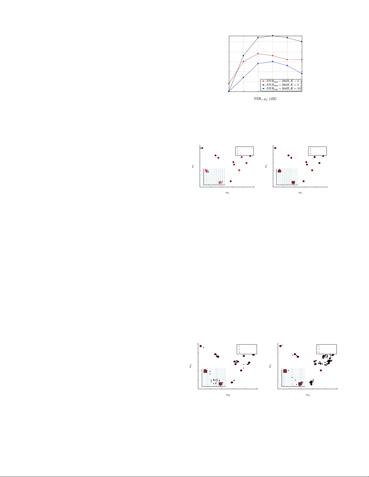
Rob ust Sparse F ourier T ransform Based on The F ourier Projection-Slice Theorem Shaogang W ang, V ishal M. P atel and Athina Petropulu Department of Electrical and Computer Engineering Rutgers, the State Univ ersity of Ne w Jersey , Piscataway , NJ 08854, USA Abstract —The state-of-the-art automotive radars employ mul- tidimensional discrete F ourier transforms (DFT) in order to estimate various target parameters. The DFT is implemented using the fast Fourier transform (FFT), at sample and com- putational complexity of O ( N ) and O ( N log N ) , respecti vely , where N is the number of samples in the signal space. W e hav e recently proposed a sparse Fourier transform based on the Fourier projection-slice theorem (FPS-SFT), which applies to multidimensional signals that are sparse in the frequency domain. FPS-SFT achieves sample complexity of O ( K ) and computational complexity of O ( K log K ) for a multidimensional, K -sparse signal. While FPS-SFT considers the ideal scenario, i.e., exactly sparse data that contains on-grid frequencies, in this paper , by extending FPS-SFT into a rob ust version (RFPS-SFT), we emphasize on addressing noisy signals that contain off-grid frequencies; such signals arise from radar applications. This is achieved by employing a windowing technique and a voting- based frequency decoding procedure; the former reduces the frequency leakage of the off-grid frequencies below the noise level to preserv e the sparsity of the signal, while the latter significantly lowers the frequency localization error stemming from the noise. The perf ormance of the pr oposed method is demonstrated both theoretically and numerically . Index T erms —Multidimensional signal processing, sparse Fourier transform, automotive radar , F ourier projection-slice theorem. I . I N T RO D U C T I O N W ith the rapid development of the advanced driv er- assistance systems (AD AS) and self-driving cars, the auto- motiv e radar plays an increasingly important role in providing multidimensional information on the dynamic environment to the control unit of the car . T raditional automotive radars mea- sure range and range rate (Doppler) of the targets including cars, pedestrians and obstacles using frequency modulation continuous wav eform (FMCW). A digital beamforming (DBF) automotiv e radar [1] can provide angular information both in azimuth and elev ation [2] of the targets, which is more desirable in the AD AS and self-dri ving applications. A typical DBF automotive radar uses uniform linear array (ULA) as the receiv e array . For such configuration and under the narrow-band signal assumption, each radar target can be represented by a D -dimensional ( D -D) complex sinusoid [3], whose frequency in each dimension relates to target param- eters, e.g., range, Doppler and direction of arriv al (DOA). The simultaneous multidimensional parameter estimation of a DBF automotiv e radar requires intensiv e processing. The con- ventional implementation of such processing relies on a D -D discrete Fourier transform (DFT), which can be implemented by the fast Fourier transform (FFT). The sample complexity of the FFT is O ( N ) , where N = Q D − 1 i =0 N i is the number of samples in the D -D data cube with N i the sample length for the i th dimension. For N a power of 2 , the computational complexity of the FFT is O ( N log N ) . Since N is typically large, the processing via FFT is still demanding for real-time processing with low-cost hardware. The recently proposed sparse Fourier transform (SFT) [4]– [6] leverages the sparsity of signals in the frequency domain to reduce the sample and computational complexity of DFT . Different v ersions of the SFT ha ve been inv estigated for sev eral applications including medical imaging, radar signal processing, etc. [7], [8]. In radar signal processing, the number of radar targets, K , is usually much smaller than N , which makes the radar signal sparse in the D -D frequency domain. Hence, it is tempting to replace the FFT with SFT in order to reduce the complexity of radar signal processing. Howe ver , most of the SFT algorithms are designed for 1-dimensional ( 1 -D) signals and their extension to multidimensional signals are usually not straightforward. This is because the SFT algo- rithms are not separable in each dimension since operations such as detection within an SFT algorithm must be considered jointly for all the dimensions [8]. Multidimensional SFT algorithms are inv estigated in [7], [9], [10]; those algorithms share a similar idea, i.e., reduction of a multidimensional DFT into a number of 1 -D DFTs. The SFT of [9] achiev es the sample and computational complexity lower bounds of all known SFT algorithms by reducing a 2 -dimensional ( 2 -D) DFT into 1 -D DFTs along ro ws and columns of a data matrix. Howe ver , such algorithm requires a very sparse signal (in the frequency domain) whose frequen- cies are uniformly distributed; such limitation stems from the restriction of applying DFT only along axes of the data matrix, which corresponds to projecting a 2 -D DFT of the data matrix onto the two axes of such matrix. In [7], [10], the multidimen- sional DFT is implemented via the application of 1 -D DFTs on samples along a few lines of predefined and deterministic slopes. Although employing lines with various slopes leads to more degrees of freedom in frequency projection of the DFT domain, the limited choice of line slopes in [7], [10] is still an obstacle in addressing less sparse signals. Moreov er , the localization of frequencies in [7], [10] is not as efficient as that of [9], which employs the phase information of the 1 -D DFTs and recovers the significant frequencies in a progressiv e manner . Thus, the SFT algorithms of [7], [10] suffer from higher complexity as compared to the SFT of [9]. W e have recently proposed FPS-SFT [11], a multidimen- sional, Fourier projection-slice based SFT , which enjoys low complexity while a voiding the limitations of the aforemen- tioned algorithms, i.e., it can handle less sparse data in the frequency domain, with frequencies non-uniformly dis- tributed. FPS-SFT uses the low-complexity frequency local- ization framew ork of [9], and extends the multiple slopes idea of [7], [10] by using lines of randomly runtime-generated slopes. The abundance of randomness of line slopes enables large degrees of freedom in frequency projection in FPS-SFT . Thus, less sparse, non-uniformly distributed frequencies can be effecti v ely resolved (see Section III-A for details). Employing random lines is not trivial, since the line parameters, including the line length and slope set should be carefully designed to enable an orthogonal and uniform frequency projection (see Lemmas 1 and 2 in [11]). FPS-SFT can be viewed as a lo w- complexity , Fourier projection-slice approach for signals that are sparse in the frequency domain. In FPS-SFT , the DFT of a 1 -D slice of the D -D data is the projection of the D -D DFT of the data to such line. While the classical Fourier projection- slice based method reconstructs the frequency domain of the signal using interpolation based on frequency-domain slices, the FPS-SFT aims to reconstruct the signal directly based on frequency domain projections; this is achiev ed by leveraging the sparsity of the signal in the frequency domain. While the FPS-SFT of [11] considered the case with exactly sparse data containing frequencies on the grid, in this paper we consider off-grid frequencies. FPS-SFT suffers from the frequency leakage caused by the of f-grid frequencies. Also, we address the noise that is contained in the signal. The frequency localization procedure of FPS-SFT is prone to error , since such low-complexity localization procedure is based on the so-called OFDM-trick [4], which is sensiti ve to noise. Addressing these issues makes the FPS-SFT more applicable to realistic radar applications where the radar signal contains off-grid frequencies and noise. W e term this new extension of FPS-SFT algorithm as RFPS-SFT . The off-grid frequencies are also addressed in [8], where we proposed a rob ust multidimensional SFT algorithm, i.e., RSFT . In RSFT , the computational savings is achiev ed by folding the input D -D data cube into a much smaller data cube, on which a reduced sized D -D FFT is applied. Although the RSFT is more computationally efficient as compared to the FFT - based methods, its sample complexity is the same as the FFT - based algorithms. Essentially , the high sample complexity of RSFT is due to its two stages of windowing procedures, which are applied to the entire data cube to suppress the frequency leakage. Inspired by RSFT , the windowing technique is also applied in RFPS-SFT to address the frequency leakage problem caused by the of f-grid frequencies. Instead of applying the multidi- mensional window on the entire data as in RSFT , the window in RFPS-SFT , while still designed for the full-sized data, is only applied on samples along lines, which does not cause ov erhead in sample complexity . T o address the frequency localization problem in FPS-SFT stemming from noise, RFPS- SFT employs a voting-based frequency localization procedure, which significantly lowers the localization error . The perfor- mance of RFPS-SFT is demonstrated both theoretically and numerically , and the feasibility of RFPS-SFT in automotive radar signal processing is shown via simulations. Notation: W e use lower-case (upper-case) bold letters to denote vectors (matrix). [ · ] T denotes the transpose of a vector . The N -modulo operation is denoted by [ · ] N . [ S ] refers to the integer set of { 0 , ..., S − 1 } . The cardinality of set S is denoted as | S | . The DFT of signal x is denoted by ˆ x . k W k 1 , k W k 2 are the l 1 and l 2 norm of matrix W , respectively . I I . S I G N A L M O D E L A N D P R O B L E M F O R M U L A T I O N W e consider the radar configuration that employs an ULA as the recei ve array . Assume that the ULA has N 1 half- wa velength-spaced elements. The radar transmits FMCW wa veform with a repetition interval (RI) of T p . W e also assume that there exist K targets in the radar coverage. After de- chirping, sampling and analog-to-digital conv ersion for both I and Q channels, the recei ved signal within an RI can be expressed as a superposition of K 2 -D complex sinusoids and noise [3], i.e., r ( n ) = y ( n ) + n ( n ) = X ( a, ω ) ∈ S ae j n T ω + n ( n ) , (1) where n , [ n 0 , n 1 ] T ∈ X , [ N 0 ] × [ N 1 ] is the sampling grid and N 0 is the number of samples within an RI. y ( n ) , P ( a, ω ) ∈ S ae j n T ω is the signal part of the received signal; ( a, ω ) represents a 2 -D sinusoid, whose complex amplitude is a , and it holds that 0 < a min ≤ | a | ≤ a max ; the 2 -D frequency ω , [ ω 0 , ω 1 ] T ∈ [0 , 2 π ) 2 represents the normalized radian frequencies corresponding to targets’ range and DO A, respectiv ely . The set S , with | S | = K contains all the 2 -D sinusoids. The noise, n ( n ) , is assumed to be i.i.d., circularly symmetric Gaussian, i.e., C N (0 , σ n ) . The SNR of a sinusoid with amplitude a is defined as S N R , ( | a | /σ n ) 2 . The tar get’ s rang r , Doppler f d and DO A θ relate to ω as ω 0 = 2 π (2 ρr /c + f d ) /f s , ω 1 = π sin θ , where ρ, c, f s are the chirp rate, the speed of wa ve propagation and sampling frequency , respectiv ely; the chirp rate is defined as the ratio of the signal bandwidth and the RI. Thus, the target parameters are embedded in frequencies ω 0 , ω 1 , which can detected in the 2 -D N 0 × N 1 -point DFT of r ( n ) [3], i.e., ˆ r ( m ) , 1 N X n ∈X w ( n ) r ( n ) e − j 2 π  m 0 n 0 N 0 + m 1 n 1 N 1  , = ˆ y ( m ) + ˆ n ( m ) , m , [ m 0 , m 1 ] T ∈ X , (2) where w ( n ) is a 2-D windo w , introduced to suppress frequency leakage generated by off-grid frequencies; N = N 0 N 1 ; and ˆ y ( m ) , ˆ n ( m ) are the DFTs of the windowed y ( n ) and n ( n ) , respecti vely . Assuming that the peak to side-lobe ratio (PSR) of the windo w is lar ge enough, such that the side- lobe (leakage) of each frequency in S can be neglected in the DFT domain, then ˆ y ( m ) is contributed by a set of 2 -D sinusoids, whose frequencies are on-grid, i.e., S 0 , { ( a, ω ) : ω , [2 π m 0 / N 0 , 2 π m 1 / N 1 ] T , [ m 0 , m 1 ] T ∈ X } with K < | S 0 | << N . Note that since the windo wing degrades the frequency resolution, each sinusoid in S is related to a cluster of sinusoids in S 0 , which can be estimated from ˆ r ( u, v ) ; next, the estimation of S can be computed from the estimation of S 0 via, for example, the quadratic interpolation method [12]. The sample domain signal component associated with the window w ( n ) , n ∈ X and the set of sinusoids, S 0 , can be expressed as x ( n ) , X ( a, ω ) ∈ S 0 ae j 2 π  m 0 n 0 N 0 + m 1 n 1 N 1  , [ n 0 , n 1 ] T ∈ X . (3) The state-of-the-art DBF automotive radars also measure the target Doppler f d by processing a 3 -dimensional ( 3 -D) data cube generated by N 2 consecutiv e RIs [3]. The normalized radian frequency ω 2 in the Doppler dimension relates to the Doppler as ω 2 = 2 π f d T p . The DBF automotiv e radars that also measure elevation DO A of targets introduce a 4 -th dimen- sion of processing [2]; the DOA measurement in elev ation is similar to that of the azimuth DO A dimension. In those cases, the proposed RFPS-SFT algorithm can be naturally extended to multidimensional cases, where the reductions of complexity of the signal processing algorithms are more significant. I I I . T H E R F P S - S F T A L G O R I T H M A. FPS-SFT The FPS-SFT algorithm proposed in [11] applies to mul- tidimensional data of arbitrary size that is exactly sparse in the frequency domain. In the 2 -D case, FPS-SFT implements a 2 -D DFT as a series of 1 -DFTs on samples extracted along lines, with each line being parameterized by the random slope parameters α , [ α 0 , α 1 ] T ∈ X and delay parameters τ , [ τ 0 , τ 1 ] T ∈ X . The signal along such line can be expressed as s ( α , τ , l ) , x ([ α 0 l + τ 0 ] N 0 , [ α 1 l + τ 1 ] N 1 ) = X ( a, ω ) ∈ S 0 ae j 2 π  m 0 [ α 0 l + τ 0 ] N 0 N 0 + m 1 [ α 1 l + τ 1 ] N 1 N 1  , l ∈ [ L ] . (4) On taking an L -point DFT on (4) w .r .t. l , we get ˆ s ( α , τ , m ) , 1 L X l ∈ [ L ] s ( α , τ , l ) e − j 2 π lm L = 1 L X ( a, ω ) ∈ S 0 ae j 2 π  m 0 τ 0 N 0 + m 1 τ 1 N 1  X l ∈ [ L ] e j 2 πl  m 0 α 0 N 0 + m 1 α 1 N 1 − m L  , m ∈ [ L ] . (5) The line length, L , which is the least common multiple (LCM) of N 0 , N 1 is designed such that the orthogonality condition for frequency projection is satisfied (see Lemma 1 of [11] for details), i.e., for m ∈ [ L ] , [ m 0 , m 1 ] T ∈ X , ˆ f ( m ) , 1 L X l ∈ [ L ] e j 2 πl  m 0 α 0 N 0 + m 1 α 1 N 1 − m L  ∈ { 0 , 1 } , (6) then if  m 0 α 0 N 0 + m 1 α 1 N 1 − m L  1 = 0 , [ m 0 , m 1 ] T ∈ X , (7) the m th entry of (5) can be simplified as ˆ s ( α , τ , m ) = P ( a, ω ) ∈ S 0 ae j 2 π  m 0 τ 0 N 0 + m 1 τ 1 N 1  . The solutions of (7) with re- spect to m lie on a line with slope − α 0 N 1 / ( α 1 N 0 ) in the N 0 × N 1 -point DFT domain (see the proof of Lemma 2 in [11]), i.e., for m 0 , m 1 satisfying (7), it holds that m 0 = [ m 0 0 + kα 1 L/ N 1 ] N 0 , m 1 = [ m 0 1 − kα 0 L/ N 0 ] N 1 , k ∈ Z , (8) where [ m 0 0 , m 0 1 ] T ∈ X is one of the solutions of (7). Hence each entry of the L -point DFT of the slice taken along a time-domain line with slope α 1 /α 0 represents a projection of the 2 -D DFT along the line with slope − α 0 N 1 / ( α 1 N 0 ) , which is orthogonal to the time-domain line. This is closely related to the Fourier projection-slice theorem. In fact, FPS-SFT can be viewed as a low-complexity , Fourier projection-slice based multidimensional DFT . This is achieved by exploring the sparsity nature of the signal in the frequency domain, which is explained in the following. Assume that the signal is sparse in the frequency domain, i.e., | S 0 | = O ( L ) . Then, if | ˆ s ( α , τ , m ) | 6 = 0 , with high probability , the m th bin is 1 -sparse, i.e., contains the projection of the DFT value from only one significant frequency , and it holds that ˆ s ( α , τ , m ) = ae j 2 π  m 0 τ 0 N 0 + m 1 τ 1 N 1  , ( a, ω ) ∈ S 0 . In such case, the 2 -D sinusoid, ( a, ω ) , can be ‘decoded’ by three lines of the same slope but different offsets. The offsets for the three lines are designed as τ , τ 0 , [[ τ 0 + 1] N 0 , τ 1 ] T , τ 1 , [ τ 0 , [ τ 1 + 1] N 1 ] T , respectively; such design allows for the frequencies to be decoded independently in each dimension. The sinusoid corresponding to the 1 -sparse bin, m , can be decoded as m 0 =  N 0 2 π φ  ˆ s ( α , τ 0 , m ) ˆ s ( α , τ , m )  N 0 , m 1 =  N 1 2 π φ  ˆ s ( α , τ 1 , m ) ˆ s ( α , τ , m )  N 1 , a = ˆ s ( α , τ , m ) e − j 2 π ( m 0 τ 0 / N 0 + m 1 τ 1 / N 1 ) . (9) T o recover all the sinusoids in S 0 , each iteration of FPS- SFT adopts a random choice of line slope (see Lemma 2 of [11]) and offset. Furthermore, the contribution of the recov ered sinusoids in previous iterations is removed to cre- ate a sparser signal. Specifically , assuming that for current iteration, the line slope and offset parameters are selected as α , τ , respectiv ely , the recovered sinusoids are projected into L frequency bins to construct the DFT along the line, ˆ s r ( α , τ , m ) , P ( a, ω ) ∈I m ae j 2 π  m 0 τ 0 N 0 + m 1 τ 1 N 1  , m ∈ [ L ] , where I m , m ∈ [ L ] represent the subsets of the recov ered sinusoids that relate to the constructed DFT along line via projection, i.e., I m , { ( a, ω ) : [ m 0 α 0 N 0 + m 1 α 1 N 1 − m L ] 1 = 0 , [ m 0 , m 1 ] T ∈ X } , m ∈ [ L ] . Next, the L -point in verse DFT (IDFT) is applied on ˆ s r ( α , τ , m ) , m ∈ [ L ] , from which the line, s r ( α , τ , l ) , l ∈ [ L ] due to the previously recovered sinusoids are constructed. Subsequently , those constructed line samples are subtracted from the signal samples of the current iteration. B. RFPS-SFT FPS-SFT [11] was developed for data that is exactly sparse in the frequency domain. Also, the frequencies are assumed to be on-grid of the N 0 × N 1 -point DFT . In the radar application howe v er , the radar signal contains noise. Also, the discretized frequencies associated with target parameters are typically off-grid. In the following, we propose RFPS-SFT , which employs the windowing technique to reduce the frequency leakage produced by the off-grid frequencies and a voting- based frequency localization to reduce the frequency decoding error due to noise. 1) W indowing: T o address the off-grid frequencies, we apply a window w ( n ) , n ∈ X on the signal of (1). The PSR of the window , ρ w , is designed such that the side-lobes of the strongest frequency are below the noise level, hence the leakage of the significant frequencies can be neglected and the sparsity of the signal in the frequenc y domain can be preserv ed to some extend. The following lemma reflects the relationship between ρ w and the maximum SNR of the signal. Lemma 1. (W indow Design): Consider (2), which is the N 0 × N 1 -point DFT of signal of (1). Let W ∈ R N 0 × N 1 be the matrix generated by the window function w ( n ) , n ∈ X . The PSR of the window , ρ w , should be designed such that ρ w > 2 k W k 1 √ π k W k 2 p S N R max , (10) Wher e S N R max , a 2 max /σ 2 n . Note that unlike the RSFT that applies windows on the entire data cube, in RFPS-SFT , while the window is still designed for the entire data cube, the windowing is applied only on the sampled locations. Thus, the windowing does not increase the sample and computational complexity of RFPS- SFT . 2) V oting-based fr equency decoding: When the signal is approximately sparse, the frequencies decoded by (9) are not integers. Since we aim to recover the gridded frequencies, i.e., S 0 of (3), the recov ered frequencies are rounded to the nearest integers. When the SNR is low , the frequency decoding could result into false frequencies; those false frequencies enter the future iterations and generate more false frequencies. T o suppress the false frequencies, motivated by the classical m -out-of- n radar signal detector [13], RFPS-SFT adopts an n d -out-of- n s voting procedure in each iteration. Specifically , within each iteration of RFPS-SFT , n s sub-iterations are ap- plied; each sub-iteration adopts randomly generated line slope and offset parameters and recovers a subset of frequencies, S i , i ∈ [ n s ] . W ithin those frequency sets, a given recovered frequency could be reco vered by n out of n s sub-iterations. F or a true significant frequency , n is typically larger than that of a false frequency , thus only those frequencies with n ≥ n d are retained as the recovered frequencies of the current iteration. When ( n s , n d ) are properly chosen, the false frequencies can be reduced significantly . 3) The lower bound of the pr obability of corr ect localiza- tion and the number of iterations of RFPS-SFT : The proba- bility of decoding error relates to the SNR, signal sparsity and choice of ( n s , n d ) in RFPS-SFT . In the following, we provide the lower bound for the probability of correct localization of the significant frequencies for each iteration of RFPS-SFT , from which one can derive the number of iterations of RFPS- SFT in order to recover all the significant frequencies of sufficient SNR. According to Section II, a 2 -D sinusoid ( a, ω ) ∈ S of (1) is associated with a cluster of 2 -D sinusoids S 0 ⊆ S 0 of (3), whose frequencies are on the grid of the N 0 × N 1 -point DFT . Let’ s assume that the sinusoid ( a d , 2 π [ m 0 / N 0 , m 1 / N 1 ] T ) ∈ S 0 with [ m 0 , m 1 ] T ∈ X has the largest absolute amplitude among the sinusoids in S 0 . In addition we assume that the SNR of ( a, ω ) is sufficiently high, then the probability of correctly localizing [ m 0 , m 1 ] T in each iteration of RFPS-SFT is lower bounded by P d , n s X n 0 d = n d  n s n 0 d  ( P 1 P w ) n 0 d (1 − P 1 P w ) n s − n 0 d , (11) where P 1 , (1 − | S 00 | / N ) N/L − 1 with L = LCM( N 0 , N 1 ) is the probability of a sinusoid in S 00 being projected to a 1 -sparse bin, and S 00 with S 00 ⊆ S 0 represents the remaining sinusoids to be recovered in the future iterations of RFPS-SFT ; P w , (1 − P u )(1 − P v ) is the lo wer bound of the probability of correct localization for a 2 -D sinusoid that is projected into a 1 -sparse bin for one sub-iteration of RFPS-SFT ; P u , P v are the upper bounds of the probability of localization error for the two frequency components, m 0 , m 1 , respectively , which is defined as P u ,  σ p (1 − f | a n | ( δ u ))  2 , P v ,  σ p (1 − f | a n | ( δ v ))  2 , where δ u , aπ k W k 1 / (2 N N 0 ) , δ v , aπ k W k 1 / (2 N N 1 ) , with W ∈ R N 0 × N 1 the windo w that is applied on the data; σ p with 1 2 ≤ σ p ≤ 1 2 π is the parameter determined by the phases of the error vectors contained in the 1 -sparse bin; f | a n | ( x ) is the cumulative distribution function (CDF) of the Rayleigh distribution, which is defined as f | a n | ( x ) , 1 − e − x 2 / (2 σ 2 a 0 n ) , x > 0 , where σ 2 a 0 n , σ 2 n k W k 2 2 / (2 N L ) . Essentially , (11) represents the complementary cumulative binomial probability resulted from the n d -out-of- n s voting procedure, where the success probability of each experi- ment, i.e., localizing ( a d , 2 π [ m 0 / N 0 , m 1 / N 1 ] T ) in each sub- iteration of RFPS-SFT is P 1 P w . When | S 0 | is kno wn, (11) can be applied to estimate the largest number of iterations (the upper bound) of RFPS-SFT in order to recover all the significant sinusoids in S 0 since the least number of recovered sinusoids in each iteration can be estimated by | S 00 | P d . 4) Complexity analysis: The RFPS-SFT executes T it- erations; within each iteration, n s sub-iterations with ran- domized line parameters are inv oked. The samples used in each sub-iteration is 3 L , since three L -length lines, with L = LCM( N 0 , N 1 ) are extracted to decode the two frequency components in the 2 -D case. Hence, the sample complexity of RFPS-SFT is O (3 T n s L ) = O ( L ) . The core processing of RFPS-SFT is the L -point DFT , which can be implemented by the FFT with computational complexity of O ( L log L ) . In addition to the FFT , each sub- iteration needs to ev aluate O ( | S 0 | ) frequencies. Hence the computational complexity of RFPS-SFT is O ( L log L + | S 0 | ) . Assuming that | S 0 | = O ( L ) , the sample and computational complexity can be simplified as O ( | S 0 | ) and O ( | S 0 | log | S 0 | ) , respectiv ely . Furthermore, since K = O ( | S 0 | ) , the sample and computational complexity of RFPS-SFT can be further simplified as O ( K ) and O ( K log K ) , respectively . 5) Multidimensional extension: The multidimensional ex- tension of RFPS-SFT is straightforward and similar to that of FPS-SFT (See Section 2 . 3 of [11] for details). I V . N U M E R I C A L R E S U LT S Effect of windowing on frequency localization: For the data that contains of f-grid frequencies, the PSR of the required window is gi v en in Lemma 1. Howe ver , the lar ger the PSR, the wider the main-lobe of the window , which results into larger frequency clusters in the DFT domain and thus larger | S 0 | (see (3)), i.e., a less sparse signal. Moreover , the larger the PSR, the smaller the SNR of the windowed signal, which leads to larger frequency localization error . Hence, for a signal with known maximum SNR, S N R max , there exists a window with the optimal PSR in terms of frequency localization success rate, i.e., ratio of number of correctly localized frequencies to the number of significant frequencies, which is | S 0 | in one iteration of RFPS-SFT . Fig. 1 shows the numerical ev aluation of such optimal windows for signals for various values of S N R max and sparsity level, i.e., K = | S | . According to (10), for signals with S N R max equal to 20 dB and 30 dB , the PSR of the windo w should be lar ger than 56 dB and 60 dB , respectiv ely . The corresponding optimal PSR for the Dolph-Chebyshev windows appear to be 60 dB and 70 dB , respectiv ely . Fig. 1 shows the success rate of the first iteration of RFPS-SFT , which is the lo west success rate of all the iterations. Fig. 2 demonstrates localization of off-grid 2 -D frequencies of RFPS-SFT using Dolph-Chebyshev window for v arious values of PSR. A windows with insufficient PSR leads to miss detections and false alarms (see Fig. 2 (a)), while a window with sufficiently large PSR yields good performance in frequency localization, with a trade-off of causing larger frequency cluster sizes (see Fig. 2 (b)). The ground truth in Fig. 2 represents (3), which relates to the window . Effect of voting on frequency localization: The n d -out-of- n s voting in frequency decoding procedure of RFPS-SFT can significantly reduce the false alarm rate. A lo w false alarm rate in each iteration of RFPS-SFT is required since the false frequencies would enter the ne xt iteration of RFPS-SFT , which creates more false frequencies. For a fixed n s , the larger the n d /n s is, the smaller the false alarm rate is. Howe ver , this in volv es a trade-off between false alarm rate and complexity; specifically , the smaller the false alarm rate, the larger the 40 50 60 70 80 90 0 0.05 0.1 0.15 0.2 0.25 Localization success rate Fig. 1. Frequency localization success rate of the first iteration of RFPS-SFT versus window PSR. The Dolph-Chebyshev windows with various PSR is applied. N 0 = N 1 = 256; ( n s , n d ) = (3 , 2) . The results are av eraged based on 100 iterations of Monte Carlo simulation. 0 50 100 150 200 250 0 50 100 150 200 250 DFT grid Ground truth Estimated 70 75 80 85 90 175 180 185 190 195 (a) 0 50 100 150 200 250 0 50 100 150 200 250 DFT grid Ground truth Estimated 70 75 80 85 90 175 180 185 190 195 (b) Fig. 2. 2 -D frequency recovery with different window . K = 10 , σ n = 1 , a min = a max , S N R max = 30 dB , ( n s , n d ) = (3 , 2) , T = 30 . Dolph-Chebyshev windows with various PSR are adopted. The ground truth represents (3), which relates to the window . A windows with insufficient PSR leads to miss detections and false alarms, while a window with sufficiently large PSR yields good performance in frequency localization, albeit resulting into larger frequency cluster size. (a) ρ w = 45 dB . (b) ρ w = 70 dB . number of the iterations required to recover all the significant frequencies. Figs. 3 and Fig. 2 (b) sho w the examples of 2 -D fre- quency recov ery using different ( n s , n d ) . In Fig. 3 (a), we set ( n s , n d ) = (1 , 1) , which reduces to the frequency localization in FPS-SFT , i.e., without voting. In this case, one can see that many false frequencies are generated. Figs. 3 (b) and Fig. 2 (b) show the frequency localization result with ( n s , n d ) equal to (3 , 1) and (3 , 2) , respectiv ely; while the former generates large amount of false frequencies, the latter exhibits ideal performance. 0 50 100 150 200 250 0 50 100 150 200 250 DFT grid Ground truth Estimated 70 75 80 85 90 175 180 185 190 195 (a) 0 50 100 150 200 250 0 50 100 150 200 250 DFT grid Ground truth Estimated 70 75 80 85 90 175 180 185 190 195 (b) Fig. 3. Effect of voting on 2 -D frequency recovery . K = 10 , σ n = 1 , a min = a max , S N R max = 30 dB . T = 30 for (a)-(c). Dolph- Chebyshev windows with ρ w = 70 dB is applied. The n d -out-of- n s voting procedure significantly improves frequency localization performance when ( n d , n s ) is properly designed. (a) ( n d , n s ) = (1 , 1) . (b) ( n d , n s ) = (3 , 1) . T ABLE I R A DA R P A RA M E T ER S Parameter Symbol V alue Center frequency f c 76 GH z Pulse bandwidth b w 200 M H z Pulse repetition time T p 89 us Number of range bins N 0 512 Number of PRI N 1 256 Number of antenna elements N 2 16 Maximum range R max 300 m Effect of the SNR and the sparsity level on the number of iterations of RFPS-SFT : The number of iterations of RFPS- SFT to recover all the significant frequencies is affected by the SNR and the sparsity lev el of the signal. A low SNR and less sparse signal requires large number of iterations. As discussed in Section III-B3, we are able to estimate the largest number of iterations that recov ers S 0 . Figs. 4 (a) shows the predicted and measured number of recovered frequencies in each iteration of RFPS-SFT for | S 0 | equal to 1000 . Fig. 4 (b) shows the predicted and measured number of iterations of RFPS-SFT for signal with various SNR and sparsity le vel. The figure shows that the number of iterations upper bounds are consistent with the measurements. 20 40 60 80 100 120 140 Iterations 0 20 40 60 80 Number of recoverd frequencies Predicted Measured (a) 200 300 400 500 600 700 800 900 1000 20 40 60 80 100 120 140 160 180 200 220 Number of iterations (b) Fig. 4. Effect of SNR and sparsity lev el on number of iterations of RFPS-SFT . (a) | S | 0 = 1000 , S N R = 30 dB , σ p = 1 / 6 . (b) Comparison of predicted and measured number of iterations for various SNR and sparsity level, | S 0 | . Radar target reconstruction: W e simulate the target re- construction for a DBF automotive radar via RFPS-SFT and compare with the RSFT . The main radar parameters are listed in T able I; such radar configuration represents a typical long- range DBF radar [3] except that we set the number of antenna elements to be moderately large to provide a better angular measurement performance. Fig. 5 shows the target reconstruc- tion of 3 radar targets via 3 -D FFT , RFPS-SFT and RSFT . All the three algorithms are able to reconstruct all the targets. Compared to the FFT and RSFT , RFPS-SFT only requires approximately 3% of data samples, which exhibits low sample complexity . Howe ver , we note that RFPS-SFT requires larger SNR than the FFT and the RSFT based methods. In near range radar applications, such as automotiv e radar , high SNR is relativ ely easy to obtain. V . C O N C L U S I O N In this paper, we hav e proposed RFPS-SFT , a rob ust ex- tension of the SFT algorithm based on Fourier projection- slice theorem. W e hav e shown that RFPS-SFT can address -20 20 0 200 DOA (degree) 15 20 150 Velocity (m/s) 40 Range (m) 100 10 50 5 FFT R-FPS-SFT RSFT (a) 43 42 20.5 5.5 Range (m) 41 21 5.4 Velocity (m/s) 40 21.5 DOA (degree) 5.3 39 22 5.2 5.1 22.5 FFT R-FPS-SFT RSFT (b) Fig. 5. Radar target reconstruction via FFT , FPS-SFT and RSFT . (a) Reconstruction of three targets. (b) Details of the frequency locations that are reconstructed for one of the three targets. multidimensional data that contains off-grid frequencies and noise, while enjoys low complexity . Hence the proposed RFPS-SFT is suitable for the low-comple xity implementation of multidimensional DFT based signal processing, such as the signal processing in DBF automotiv e radar . R E F E R E N C E S [1] M. Schneider , “ Automotive radar-status and trends, ” in German mi- cr owave conference , pp. 144–147, 2005. [2] K. Shirakawa, S. Kobashi, Y . Kurono, M. Shono, and O. Isaji, “3d-scan millimeter-wa ve radar for automotive application, ” Fujitsu T en T ech. J , vol. 38, pp. 3–7, 2013. [3] F . Engels, P . Heidenreich, A. M. Zoubir, F . K. Jondral, and M. Win- termantel, “ Adv ances in automotiv e radar: A framework on compu- tationally efficient high-resolution frequency estimation, ” IEEE Signal Pr ocessing Magazine , vol. 34, no. 2, pp. 36–46, 2017. [4] H. Hassanieh, P . Indyk, D. Katabi, and E. Price, “Nearly optimal sparse Fourier transform, ” in Pr oceedings of the forty-fourth annual A CM symposium on Theory of computing , pp. 563–578, ACM, 2012. [5] A. C. Gilbert, P . Indyk, M. Iwen, and L. Schmidt, “Recent developments in the sparse Fourier transform: A compressed Fourier transform for big data, ” Signal Processing Magazine, IEEE , vol. 31, no. 5, pp. 91–100, 2014. [6] S. Pawar and K. Ramchandran, “FF AST : An algorithm for computing an exactly k-sparse DFT in O(klogk) time, ” IEEE T ransactions on Information Theory , vol. PP , no. 99, pp. 1–1, 2017. [7] H. Hassanieh, M. Mayzel, L. Shi, D. Katabi, and V . Y . Orekhov , “Fast multi-dimensional NMR acquisition and processing using the sparse FFT, ” Journal of Biomolecular NMR , pp. 1–11, 2015. [8] S. W ang, V . M. Patel, and A. Petropulu, “ A robust sparse fourier trans- form and its application in radar signal processing, ” IEEE T ransactions on Aer ospace and Electr onic Systems , 2017. [9] B. Ghazi, H. Hassanieh, P . Indyk, D. Katabi, E. Price, and L. Shi, “Sample-optimal av erage-case sparse Fourier transform in two dimen- sions, ” in Communication, Contr ol, and Computing (Allerton), 2013 51st Annual Allerton Conference on , pp. 1258–1265, IEEE, 2013. [10] L. Shi, H. Hassanieh, A. Davis, D. Katabi, and F . Durand, “Light field reconstruction using sparsity in the continuous Fourier domain, ” ACM T ransactions on Graphics (TOG) , vol. 34, no. 1, p. 12, 2014. [11] S. W ang, V . M. Patel, and A. Petropulu, “FPS-SFT : A Multi- dimensional Sparse Fourier T ransform Based on the Fourier Projection-slice Theorem, ” Submitted to ICASSP 2018. A valiable at: http://eceweb1.rutgers.edu/ cspl/publications/fps-sft-multi.pdf. [12] J. O. Smith and X. Serra, P ARSHL: An analysis/synthesis pro gram for non-harmonic sounds based on a sinusoidal repr esentation . CCRMA, Department of Music, Stanford University , 1987. [13] M. I. Skolnik, Radar handbook . McGraw-Hill Education, 3rd ed., 2008.