Utilizing Domain Knowledge in End-to-End Audio Processing

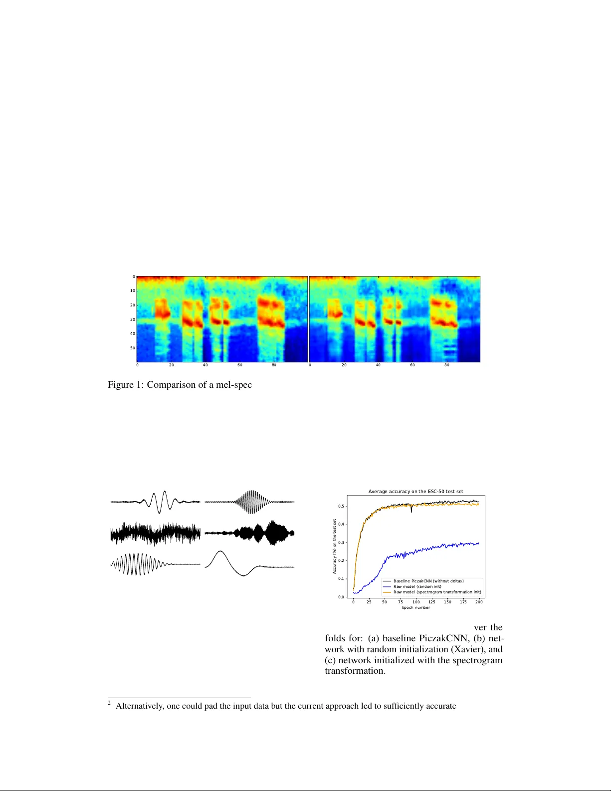
Utilizing Domain Knowledge in End-to-End A udio Pr ocessing T ycho Max Sylvester T ax Corti, Copenhagen, Denmark tt@cortilabs.com Jose Luis Diez Antich Audio Analysis Lab, Aalborg Uni v ersity Copenhagen jl.diez.antich@gmail.com Hendrik Purwins Audio Analysis Lab, Aalborg Uni v ersity Copenhagen hpu@create.aau.dk Lars Maaløe Corti, Copenhagen, Denmark T echnical Univ ersity of Denmark lm@cortilabs.com Abstract End-to-end neural network based approaches to audio modelling are generally outperformed by models trained on high-le v el data representations. In this paper we present preliminary w ork that sho ws the feasibility of training the first layers of a deep conv olutional neural network (CNN) model to learn the commonly- used log-scaled mel-spectrogram transformation. Secondly , we demonstrate that upon initializing the first layers of an end-to-end CNN classifier with the learned transformation, con ver gence and performance on the ESC-50 en vironmental sound classification dataset are similar to a CNN-based model trained on the highly pre-processed log-scaled mel-spectrogram features. 1 Introduction End-to-end neural network models on image recognition tasks outperform other machine learning approaches by a lar ge margin [ 11 ] b ut similarly good results are not seen in the audio domain. Modeling audio is particularly challenging because of long-range temporal dependencies [ 13 ] and variations for the same sound due to temporal distortions and phase shifts [ 5 ]. V arious papers within automatic speech recognition (ASR), audio classification, and speech synthesis attempt to model audio from raw w av eform [ 3 ][ 13 ][ 8 ][ 2 ]. Combinations of autoregressiv e models and dilated con v olutions hav e shown significant impro vements o ver pre vious results [ 13 ]. Still, on tasks such as ASR and en vironmental sound classification, using traditional transformations, such as (log-scaled mel-)spectrograms or MFCCs generally leads to superior performance. Modern neural netw ork models are initialized using network-architecture-dependent randomized schemes [ 7 ][ 6 ]. In this paper we present preliminary work on initializing a deep neural network for audio classification by explicitly lev eraging domain kno wledge instead. T o do so, we first sho w that it is possible to train the first layers of a deep neural network model, using unlabelled data, to learn a high-lev el audio representation. Secondly , we sho w that upon initializing the first layers of an end-to-end environmental sound classifier with the learned transformation, and keeping the associated parameters fixed during training, con v ergence and performance are similar to that of a model trained on the high-lev el representation. This opens up the possibility for training end-to-end neural network models on raw w av eform in contexts where there is a limited amount of labeled data av ailable. Finally , we discuss several future directions. It will be particularly interesting to see if fine-tuning of the model after con ver gence by unfreezing the parameters of the first layers can allo w the performance of models trained on raw wa v eform to surpass those trained on processed features. 31st Conference on Neural Information Processing Systems (NIPS 2017), Long Beach, CA, USA. 2 Sound classification 2.1 Dataset and baseline results Sev eral datasets have been generated in recent years to address the pre viously limited av ailability of labeled en vironmental sound data [ 17 ][ 4 ][ 15 ]. Of particular interest is the En vironmental Sound Classification (ESC) dataset, which was released by Piczak in 2015 along with reproducible baseline results for se veral standard machine learning classifiers (k-NNs, SVMs and RF ensembles) [ 15 ] as well as for a con volutional neural network model, which we denote as the PiczakCNN [ 14 ], and which we use as a baseline for our study . For our analysis, we use the ESC-50 dataset [ 15 ], which contains 2000 5-second long audio clips equally di vided among 50 cate gories. The recordings are pre-arranged in fiv e equally sized folds to facilitate cross-v alidation. The PiczakCNN consists of two 2-D CNN layers interlea ved with max-pooling follo wed by two fully connected layers and a softmax output layer . It uses segmented log-scaled mel-spectrograms alongside their deltas as input. The reader is referred to the original paper for more details [ 14 ]. In line with Piczak, we increase the ef fectiv e number of training samples by making four v ariations of each ESC-50 clip using time-/pitch-shifting. In addition, each of the mel-spectrograms is cut into segments of 101 frames with 50% ov erlap, and silent segments are discarded. At test time, a label is predicted for each of the se gments associated with a clip and majority or probability voting is used to determine the final predicted class. Using majority v oting the PiczakCNN model achie ves a ∼ 62% accuracy on the test set a veraged o ver the fi v e folds [14]. Since we are interested in an end-to-end approach we add sev eral 1-D CNN layers to the PiczakCNN architecture to allow raw wav eform as input 1 . These layers by themselves form the model that is trained separately to learn the mel-spectrogram transformation after which the learned weights are used to initialize the end-to-end classifier and kept frozen for the classification task. For this study , we first replicate Piczak’ s results using mel-spectrograms and their deltas to ensure that our set-up performs adequately . As we attempt to learn the mel-spectrogram transformation only , and not also the associated deltas, we benchmark our results on raw speech against PiczakCNN performance without deltas, which is ∼ 53% on the test set using majority voting, and a veraged o ver the 5 folds. 2.2 Learning the mel-spectr ogram transf ormation 2.2.1 Experimental set-up After exploring se veral architectures for the mel-spectrogram transformation model (MSTmodel) we picked the architecture summarized in T able 1. The reason is twofold: firstly , it sho ws excellent performance on the modelling task, and secondly , its parameters are matched in terms of kernel size and stride to the window-and hop-size of the short-time Fourier transform (STFT) step in the mel-spectrum calculation. The second and third layer are qualitativ ely similar to those used for temporal modelling in [ 2 ]. ’SAME’ padding is used in the MSTmodel so that the output feature maps are of the same spatial dimension as the input feature maps in order not to lose information at the edges of the signal during the forward pass. T able 1: Details of the MSTmodel. Layer type Number of filters Filter size Stride Activ ation function Padding 1D con v olution 512 1024 512 ReLU SAME 1D con v olution 256 3 1 ReLU SAME 1D con v olution 60 3 1 T anh SAME The MSTmodel is trained stand-alone, in supervised fashion, by taking ra w audio clips as input and their corresponding mel-spectrograms as labels. The raw wa veform recordings are re-sampled at 22050Hz from their original 44.1kHz, and their amplitudes are normalized per segment (correspond- ing to a single mel-spectrogram of framelength 101) between -1 and 1 through di vision with the maximum absolute v alue of the se gment. A target mel-spectrogram is generated using the Librosa 1 Source code for the project will be made av ailable at: https://github.com/corticph/MSTmodel . 2 package [ 12 ] by applying a mel-filterbank to the magnitude spectrum of each segment (windo w size = 1024, hop size = 512, and mel bands = 60), and then taking its log arithm. The mel-spectrogram values are normalized and re-scaled between -1 and 1 using trainset statistics. T o train the MSTmodel we use a simple mean squared error (MSE) loss between the predicted representations and the tar get mel-spectrograms, where the last frame of each label is sliced of f to match dimensions 2 . W e use Adam [ 10 ] with a constant learning rate ( 3e − 4 ) and a batch size of 100 for optimization, and prev ent o verfitting through early stopping based on the performance on the pre-allocated validation set. Separate models are trained for each pre-assigned fold to ensure that upon initializing the end-to-end classifier , it has not pre viously ’ seen’ test or validation data. 2.2.2 Results and discussion Figure 1 shows the learned mel-spectrogram (right) and its target (left) for a randomly selected example from the test set. The prediction is visually similar to the target although the spectrum seems slightly smoothed. W e hav e verified the learned transformation is not domain dependent by comparing the model predictions with their targets on pure tones, speech, and music. 0 20 40 60 80 0 10 20 30 40 50 0 20 40 60 80 Figure 1: Comparison of a mel-spectrogram (left) and its prediction (right). The signal is randomly chosen from the test set. In Figure 2, we plot some of the learned filters of the first layer of the MSTmodel. It can be seen that our network learns frequenc y decompositions such as wa velets and band-pass filters that are qualitativ ely similar to those reported in previous studies [ 18 ][ 1 ][ 8 ]. It is interesting that our network discov ers the same representations despite being trained on a different task. Figure 2: Subset of the filters learned by the first MSTmodel layer . 0 25 50 75 100 125 150 175 200 Epoch number 0.0 0.1 0.2 0.3 0.4 0.5 Accuracy (%) on the test set Average accuracy on the ESC-50 test set Baseline PiczakCNN (without deltas) Raw model (random init) Raw model (spectrogram transformation init) Figure 3: T est accuracy av eraged ov er the folds for: (a) baseline PiczakCNN, (b) net- work with random initialization (Xavier), and (c) network initialized with the spectrogram transformation. 2 Alternativ ely , one could pad the input data b ut the current approach led to suf ficiently accurate mel-spectro- grams for our purposes. 3 2.3 End-to-end en vir onmental sound classification 2.3.1 Experimental set-up W e assess the success of learning the mel-spectrogram transformation by performance on the ESC- 50 dataset. T o do so, we train three models, where in each case we adhere to the pre-defined cross-validation structure for the ESC-50 dataset [ 14 ]: 1. the baseline PiczakCNN model on mel- spectrograms without deltas, 2. the PiczakCNN model with the three-layer MSTmodel architecture added, and with random initialization using the Xavier scheme [ 6 ], and 3. the same model as in 2 but with the pre-trained MSTmodel layers. In the second classifier , dropout layers (keep probability = 0.5) are added to the MSTmodel-layers after each of the non-linearities to pre vent overfitting. For the third classifier we keep the MSTmodel parameters frozen to the learned mel-spectrogram transformation during training of the deeper layers. The training scheme used is largely the same as the one proposed by Piczak [ 14 ] with minor adaptions to the hyperparameter choices and normalization—after normalization the mel-spectrogram v alues are re-scaled between -1 and 1 based on the minimum and maximum of the trainset. W e use a cross-entropy loss function and stochastic gradient descent with Nestero v momentum (0.9), a batch size of 500, and a learning rate of 5e − 3 , and we train the models for 200 epochs. The originally proposed L2-weight regularization is not used in the final e xperiments since it did not improv e performance. At test-time, majority v oting is used to determine the class of the test sample based on all its associated ov erlapping segments. 2.3.2 Results and discussion The performance of the three models outlined above is presented in Figure 3 on the test set a veraged ov er the fi v e folds. W e see that initializing the weights of the first layers with the learned mel- spectrogram transformation, and keeping them fix ed throughout training, results in better con vergence and increases performance on raw wa v eform approximately to mel-spectrogram-lev els. When using neural networks for audio modelling, architectural choices are sometimes made that appear inspired by deterministic feature extracting methods. For instance, max-pooling is often used to perform a summarizing process comparable to the mel-filter bank operating on a mel-spectrogram. In addition, log-layers are sometimes used to compress the learned internal representation [ 16 ][ 8 ]. CNNs are highly flexible models that can approximate complex mappings. By le veraging this capability in our approach, and forcing the network to learn such transformations implicitly , we limit the need for ad-hoc architectural choices. 3 Conclusion and future dir ections This proof-of-concept study sho ws that 1) through supervised training, a simple CNN architecture can learn the log-scaled mel-spectrogram transformation from raw w av eform and 2) that initializing an end-to-end neural network classifier with the learned transformation yields a performance comparable to a model trained on the highly processed mel-spectrograms. These findings show that incorporating knowledge from established audio signal processing methods can improve performance of neural network based approaches on audio modeling tasks. This preliminary work opens up the possibility for a myriad of follow-up experiments. Most notably , it will be interesting to fine-tune the previously fixed parameters of the first layers of the classifier to determine if dif ferent representations are learned and whether they are more informativ e than mel-spectrograms. If so, the rob ustness of these representations can be further increased through an abundance of a vailable unlabelled audio data. This parallels work by Jaitly and Hinton who use generative models to lev erage unlabeled data to learn robust features [9]. Acknowledgments The authors would lik e to thank Karol Piczak for making the code to reproduce his baseline results publicly a vailable, and for answering sev eral questions relating the ESC dataset. In addition, we would like to thank the Corti team, Lasse Borgholt and Ale xander W ahl-Rasmussen in particular , for insightful feedback, and proofreading the manuscript. 4 References [1] Y . A ytar , C. V ondrick, and A. T orralba. Soundnet: Learning sound representations from unlabeled video. In Advances in Neural Information Pr ocessing Systems , pages 892–900, 2016. [2] R. Collobert, C. Puhrsch, and G. Synnae ve. W av2letter: an end-to-end con vnet-based speech recognition system. arXiv pr eprint arXiv:1609.03193 , 2016. [3] S. Dieleman and B. Schrauwen. End-to-end learning for music audio. In IEEE International Confer ence on Acoustics, Speech and Signal Pr ocessing (ICASSP) , pages 6964–6968, 2014. [4] J. F . Gemmek e, D. P . W . Ellis, D. Freedman, A. Jansen, W . Lawrence, R. C. Moore, M. Plakal, and M. Ritter . Audio set: An ontology and human-labeled dataset for audio ev ents. In IEEE International Confer ence on Acoustics, Speech and Signal Pr ocessing (ICASSP) , 2017. [5] P . Ghahremani, V . Manohar , D. Po vey , and S. Khudanpur . Acoustic modelling from the signal domain using cnns. In INTERSPEECH , pages 3434–3438, 2016. [6] X. Glorot and Y . Bengio. Understanding the difficulty of training deep feedforward neural networks. In Pr oceedings of the Thirteenth International Confer ence on Artificial Intelligence and Statistics , volume 9, pages 249–256, 2010. [7] K. He, X. Zhang, S. Ren, and J. Sun. Delving deep into rectifiers: Surpassing human-level performance on imagenet classification. Pr oceedings of the IEEE international confer ence on computer vision , 2015. [8] Y . Hoshen, R. J. W eiss, and K. W . W ilson. Speech acoustic modeling from raw multichannel wa veforms. In IEEE International Confer ence on Acoustics, Speech and Signal Processing (ICASSP) , pages 4624–4628, 2015. [9] N. Jaitly and G. Hinton. Learning a better representation of speech soundwa v es using restricted boltzmann machines. In IEEE International Conference on Acoustics, Speech and Signal Pr ocessing (ICASSP) , pages 5884–5887, 2011. [10] D. Kingma and J. Ba. Adam: A method for stochastic optimization. arXiv preprint arXiv:1412.6980 , 2014. [11] A. Krizhevsk y , I. Sutske ver , and G. E. Hinton. Imagenet classification with deep con volutional neural networks. In Advances in Neural Information Processing Systems , pages 1097–1105. 2012. [12] B. McFee, M. McV icar, O. Nieto, S. Balke, C. Thome, D. Liang, E. Battenberg, J. Moore, R. Bittner , R. Y amamoto, D. Ellis, F .-R. Stoter , D. Repetto, S. W aloschek, C. Carr , S. Kranzler , K. Choi, P . V iktorin, J. F . Santos, A. Holov aty , W . Pimenta, and H. Lee. librosa 0.5.0, 2017. [13] A. v . d. Oord, S. Dieleman, H. Zen, K. Simon yan, O. V inyals, A. Grav es, N. Kalchbrenner , A. Senior , and K. Ka vukcuoglu. W avenet: A generati ve model for raw audio. arXiv pr eprint arXiv:1609.03499 , 2016. [14] K. J. Piczak. Environmental sound classification with con v olutional neural networks. In Ma- chine Learning for Signal Pr ocessing (MLSP), IEEE 25th International W orkshop on Machine Learning for Signal Pr ocessing , pages 1–6, 2015. [15] K. J. Piczak. Esc: Dataset for en vironmental sound classification. In Pr oceedings of the 23r d A CM international confer ence on Multimedia , pages 1015–1018, 2015. [16] T . N. Sainath, R. J. W eiss, A. Senior, K. W . Wilson, and O. V inyals. Learning the speech front-end with raw wa veform cldnns. In Sixteenth Annual Confer ence of the International Speech Communication Association , 2015. [17] J. Salamon, C. Jacoby , and J. P . Bello. A dataset and taxonomy for urban sound research. In Pr oceedings of the 22nd ACM international confer ence on Multimedia , pages 1041–1044, 2014. [18] Z. Tüske, P . Golik, R. Schlüter , and H. Ney . Acoustic modeling with deep neural networks using ra w time signal for lvcsr . In F ifteenth Annual Confer ence of the International Speech Communication Association , 2014. 5