Cognitive Networks Achieve Throughput Scaling of a Homogeneous Network

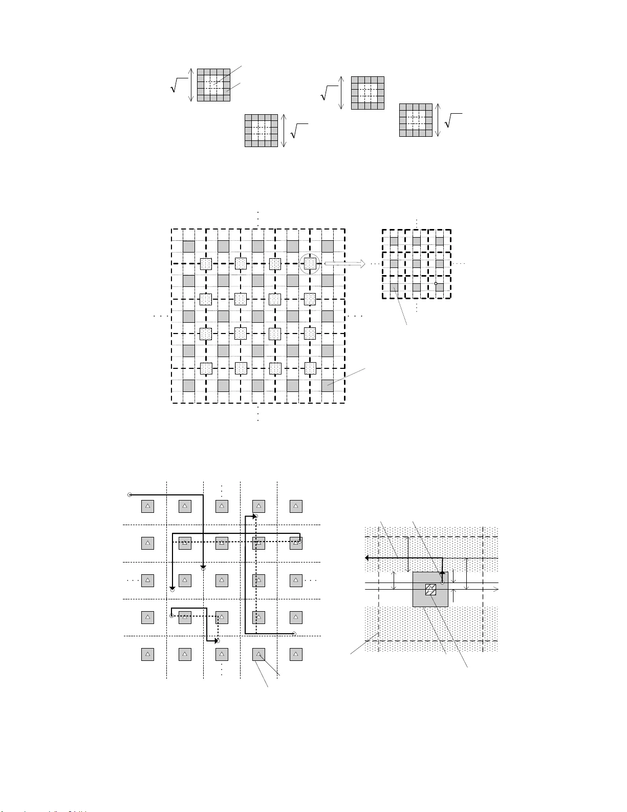
1 Cogniti v e Netw orks Achie v e Throughp ut Scaling of a Homogeneous Netw ork Sang-W oon Jeon, Student Member , I EEE , Natasha De vroye, Mai vu, Member , IEEE Sae-Y oung Chung, Senior Member , IEEE , and V ahid T arokh F ell ow , IEEE Abstract W e study two distinct, but ov erlappin g, networks that operate at the same time, space, an d frequency . Th e ﬁrst network con sists of n random ly distributed primary u sers , which form either an ad h oc n etwork, or an infrastructure - supported ad h oc network with l a dditional base stations. The second network con sists of m r andomly distributed, ad hoc seco ndary users or cognitive users . The primary users h av e priority access to the spectrum and do no t need to change their comm unication protoco l in the p resence of secondar y users. The secondary users, howev er , nee d to adjust their protoco l based on knowledge ab out the loca tions o f the prim ary nod es to bring little loss to the primary network’ s thro ughp ut. By introd ucing preservation region s around primary rec eiv ers and av o idance r egions around pr imary base stations, we propose two modiﬁed multihop r outing p rotoco ls for th e cognitive u sers. Base on percolation th eory , we show that when th e seco ndary n etwork is denser than the p rimary n etwork, bo th n etworks can simultaneou sly achieve the same throug hput scaling la w as a stand-alone n etwork. Fu rthermo re, the primary network throug hput is subject to only a vanishingly fractional loss. Speciﬁcally , for the ad hoc and the infrastructure-su pported primary m odels, the pr imary network achieves sum th rough puts of or der n 1 / 2 and ma x { n 1 / 2 , l } , r espectiv ely . For both primary network mo dels, for any δ > 0 , the seconda ry network can achieve sum throug hput o f ord er m 1 / 2 − δ with an arbitrarily small fractio n of outage. Thu s, almost all seco ndary so urce-de stination p airs can commu nicate at a r ate of ord er m − 1 / 2 − δ . Index T er ms Cognitive radio, scaling law , heterogen eous network s, interferen ce man agement, routing algo rithm I . I N T RO D U C T I O N In the ir pioneering work [1], Gupta and Kumar posed and studied the limits of communication in ad hoc wireless networks. Ass uming n nodes a re uniformly distributed in a plane a nd g rouped into source -destination (S-D) pairs at ran dom, they showed that one ca n achieve a sum throughput of S ( n ) = Θ ( p n/ log n ) . This is ach iev ed using a multihop transmission scheme in which nodes transmit to one of the nodes in their neighbo ring cells, requiring full connec ti vity with at least one n ode per cell. A trade-off between throughput and delay o f fully-connected networks was studied in [2] and was exten ded in [3] to trade-offs betwee n throughput, de lay as well as ene r gy . The work in [4] has studied relay networks in which a single source transmits its da ta to the intended destination using the othe r nod es a s relays. Us ing percolation theo ry [5], [6], they showed that a con stant rate is achiev able for a single S-D pa ir if we allow a small fraction of no des to be disconn ected. T his result can be ap plied to ad hoc ne tworks having multiple S-D pairs a nd the work in [7] propos ed an indirect mu ltihop routing protoc ol based on suc h partial conn ectivit y , that is all S-D pairs perform mu ltihop transmissions bas ed on this pa rtially- connec ted sub-network. They showed that the indirect multihop routing improves the achiev able sum throughput as S ( n ) = Θ( √ n ) . Information-theoretic outer bo unds on throughp ut sca ling laws of a d hoc wireless ne tworks were d eri ved in [8], [9], [10], [11]. Th ese bounds sh owed that the multihop routing using neighb or nod es is o rder- optimal in the power- limited an d high attenua tion regime. Rec ently , a hierarchica l coo peration scheme was propos ed in [12 ] and was S.-W . Jeon and S.-Y . Chun g are with the School of EECS , KAIST , Daejeon, Korea (e-mail: swjeon@kaist.ac.kr; sych ung@ee.kaist.ac.kr). N. De vroye is with the Dept. of Electrical and Compu ter Engineering, Uni versity of Illinois at Chicago, Chicago , IL 60607 USA (e-mail: de vroye@u ic.edu). M. V u is with the Department of El ectrical and Computer Engineering, McGill University , Montreal, Canada (e-mail: mai.h.vu@mcgill.ca). V . T arohk is with the School of Engineering and Applied Sciences, Harv ard Uni versity , Cambridge, MA 02138 US A (e-mail: v ahid@seas.harv ard.edu). The material in this paper was presented in part at the 7th I nternational Symposium on Mode ling and Optimization in Mobile, Ad Hoc, and Wireless Networks (W iOpt), Seoul, K orea, June 2009. 2 shown to ac hieve better throughpu t sc aling than the multihop strategy in the interference-limited or low attenua tion regime, a chieving a scaling very clos e to their ne w outer boun d. A more ge neral hierarchical cooperation was proposed in [13 ], which works for an arbitrary node distrib ution in which a minimum se paration b etween no des is guaranteed . Recently hybrid network mode ls ha ve bee n s tudied as well. Hybrid networks are ad hoc networks in wh ich the n odes’ c ommunication is a ided by ad ditional infrastructures su ch as b ase s tations (BSs). Thes e are gen erally assume d to have high ban dwidth connections to e ach other . In [14], [15] the connec ti vity of hybrid networks has been an alyzed. In [16], [17], [18], [19], [20] the throughput sc aling of hyb rid networks has been s tudied. In order for a hyb rid network’ s throu ghput scaling to o utperform that of a s trictly ad hoc ne twork, it was determined that the number of BSs shou ld b e grea ter than a c ertain thresho ld [17], [19]. The existing literatures have foc used on the throughp ut scaling of a s ingle network. Ho wever , the necess ity of extending and expan ding results to c apture multiple overlapping networks is becoming apparen t. Recen t mea- surements have shown tha t des pite increa sing de mands for bandwidth, much of the currently license d s pectrum remains unused a surprisingly lar ge portion of the time [21]. In the US, this has led the Federal Communications Commission (FCC) to c onsider eas ing the regulations tow ards sec ondary spectr um sharing through their S econda ry Markets Initiative [22]. The essenc e of second ary sp ectrum sh aring in volves having primary license holde rs allow second ary license holders to ac cess the spectrum. Different types of sp ectrum sh aring exist but most ag ree that the primary users have a highe r priority acces s to the spe ctrum, while seco ndary users opportunistically us e it. These second ary users often require greater sensing abilities and mo re ﬂexible an d di verse commun ication abilities than legacy primary users. Seco ndary users are often assume d to be c ognitive rad ios , or wireless devices which a re able to transmit a nd receive ac cording to a variety of protocols an d are also able to se nse and inde pende ntly a dapt to their en vironment [23]. These features a llo w them to be have in a more “intelligent” manner than cu rrent wireless devices. In this pap er , we c onsider c ognitive networks , which consist of sec ondary , or co gniti ve, users who wish to transmit over the s pectrum licensed to the primary use rs. The single-us er ca se in wh ich a s ingle primary and a single c ognitiv e S-D pairs s hare the spectrum has been conside red in the literature, se e for example [24], [25], [26], [27] and the references therein. In [24] the primary and cognitiv e S-D pairs are modeled as an interference channe l with asymmetric side-information. In [26] the communication op portunities are modeled as a two-switch cha nnel. Recently , a single-hop cognitiv e network was co nsidered in [28], where multiple sec ondary S-D pairs transmit in the presence of a single primary S-D pair . It was shown that a linear s caling law of the single-hop s econda ry network is o btained wh en its operation is constrained to guarantee a particular outage con straint for the p rimary S-D pa ir . W e study a more general en vironment in which a primary a d ho c networ k a nd a cognitive ad hoc network both sh are the same space, time and freque ncy d imensions. T wo types o f primary networks are conside red in this paper : a n ad hoc primary network and an infrastructure-supported primary ne twork. For the ad hoc primary model, the primary network consists of n node s ra ndomly distribut ed a nd grouped into S-D pairs at random. For the infrastructure-supported p rimary model, additional l BSs are regularly d eployed an d u sed to support the primary transmissions. In b oth cas es, the cogn iti ve ne twork consists of m secon dary nodes distributed randomly and S -D pairs are a gain chos en randomly . Our main a ssumptions are that (1) the primary ne twork continues to o perate as if no se conda ry n etwork were present, (2) the sec ondary nod es know the locations of the primary n odes an d (3) the second ary network is dens er than the primary ne twork. Under these ass umptions, we will illustrate routing protocols for the primary a nd s econda ry ne tworks that res ult in the s ame thr oughpu t sca ling as if eac h were a s ingle ne twork. Note that the constraint that the primary n etwork does not alter its protocol beca use of the se condary network is what makes the problem non -tri vial. Indeed, if the p rimary network were to chan ge its protoc ol whe n the s econda ry network is present, a simple time-sharing sc heme is able to achieve the through put scaling of homog eneous networks for both primary and sec ondary networks. For the ad hoc primary mode l, we use a routing protocol that is a simple modiﬁcation of the neares t ne ighbor multihop schemes in [1 ], [7]. For the infrastructure-supported primary model, we use a BS-bas ed tr ansmiss ion similar to the scheme in [17]. W e propose n ovel routing protocols for the secondary network unde r ea ch primary network model. Our proposed protocols us e multihop routing, in which the secondary routes avoid pass ing too close to the p rimary nodes, redu cing the interference to them. W e show that the propos ed protocols ach iev e the throughput scalings of homogen eous networks simultaneously . This implies that when a dens er “intelligent” network 3 is layered on top of a sparse r obli vious one , then both may a chieve the sa me throughput sc alings as if eac h were a single network. This res ult may be extend ed to more than two n etworks, provided each layered network obeys the same three main assumptions as in the two network case . This p aper is s tructured a s follows. In Section II we outline the s ystem mode l: we ﬁrst look at the network geometry , c o-existing primary and s econda ry a d h oc networks, then turn to the information theoretic achievable rates before stating o ur as sumptions on the primary and se conda ry network b ehaviors. In Section III we o utline the protocols used for the a d hoc primary model a nd prove tha t the c laimed single network throughput s calings may be achieved. W e also prove the claimed single ne twork throug hput scalings for the infrastructure-suppo rted primary mod el in Section IV. W e conclude in Section V and refer the proofs of the lemmas to the Append ix. I I . S Y S T E M M O D E L In orde r to study throughp ut scaling laws of ad ho c cognitive networks, we must deﬁn e the underlying network models. W e ﬁrst explain the two geometric mode ls that will b e considered in Sec tions III and IV. W e then look at the transmiss ion s chemes , resulting achievable rates, and a ssumptions mad e abo ut the primary and seco ndary networks. Throughou t this pa per , we u se P ( E ) to denote the p robability o f a n event E and we will b e de aling with events which take place with high prob ability (w .h.p.), o r with probability 1 as the node density tends to inﬁnity 1 . A. Network Geometry W e c onsider a plana r area in which a ne twork of primary nodes and a network of sec ondary n odes co-exist. That is, the two ne tworks share the same spac e, time, code, and frequency dimen sions. T wo types of networks a re considered as the primary n etwork: an ad hoc network and an infrastructure-supported network , while the sec ondary network is alw ays ad ho c. The two geome tric models are illustrated in Fig. 1. As shown in Fig. 1. (a), in the ad hoc primary model, nodes are distributed ac cording to a P oisson point process (p.p.p.) of de nsity n over a un it square, which are randomly g rouped into primary S-D pairs. For the s econd ary network, nodes are distributed acc ording to a p.p.p . o f de nsity m over the same unit square a nd are also rando mly groupe d into s econda ry S-D pa irs. Our se cond model is the infrastructure-suppo rted primary mode l, shown in Fig. 1. (b). There, primary n odes are still randomly distrib uted over the square a ccording to a p.p.p. of dens ity n , but the se n odes are suppo rted by additional l regularly spac ed BSs (the numbe r of BSs is equal to l , which is also the density of BSs). The BSs’ sole purpose is to relay data for the primary network, they a re neither sources nor de stinations. W e assu me that the BSs are con nected to eac h other through wired lines o f ca pacity lar ge enough such that the BS-BS communication is not the limiting factor in the throughput scaling laws. Secondary no des again form a n ad hoc network w ith random S-D pa irs, distributed acc ording to a p.p. p. of d ensity m . The d ensities of the n primary n odes, m seco ndary nodes, a nd l BSs are related acc ording to n = m 1 β = l 1 γ , (1) where β > 1 and γ < 1 . W e focus on the cas e wh ere the density of the se condary node s is higher than that o f the primary nodes. W e also ass ume that the densities of both the p rimary no des and sec ondary nod es a re h igher than that o f the BSs, wh ich is reasona ble from a prac tical point of view . The wir eless propagation channe l typically includes path l oss wit h distance, shad owing an d fading ef fects. Howe ver , in this work we assume the channel g ain d epends only on the distance be tween a transmitter an d its receiv er , an d ignore shadowing and fading. Thus, the c hannel power gain g ( d ) , normalized by a constant, is given by g ( d ) = d − α , (2) where d denotes the distanc e betwee n a trans mitter (Tx) and its receiver (Rx) an d α > 2 d enotes the pa th-loss exponent. 1 For simplicity , we use the notation w .h.p. in the paper to mean an even t occurs with high probability as n → ∞ . 4 B. Rates and Throughputs Achieved Each network o perates based on s lotted transmissions. W e assume the duration of each slot, and the c oding scheme employed are s uch that o ne can achieve the additi ve white Gau ssian noise (A WGN) chan nel ca pacity . For a gi ven signal to interference and no ise ratio (SINR), this ca pacity is g i ven by the well known formula R = log (1 + SINR) bps/Hz ass uming the additi ve interference is also white, G aussian , and ind epende nt from the no ise and signa l. W e assume tha t primary slots an d sec ondary slots have the same duration an d are syn chronized with e ach other . W e further as sume all the primary , secondary , a nd BS nodes are subject to a trans mit po wer con straint P . W e now c haracterize the rates ac hieved by the primary and secon dary transmit pairs. Suppose that N p primary pairs and N s second ary pairs commu nicate simultaneous ly . Before p roceeding with a detailed desc ription, let us deﬁne the notations used in the paper , given b y T able I. Then, the i -th primary pair c an commun icate at a rate of R i p = log   1 + P i p g  k X i p, tx − X i p, rx k  N 0 + I i p + I i sp   , (3) where k · k de notes the Euclidean norm of a vector . I i p and I i sp are given by I i p = N p X k =1 ,k 6 = i P k p g  k X k p, tx − X i p, rx k  (4) and I i sp = N s X k =1 P k s g  k X k s, tx − X i p, rx k  . (5) Similarly , the j -th sec ondary pair can commun icate at a rate of R j s = log   1 + P j s g  k X j s, tx − X j s, rx k  N 0 + I j s + I j ps   , (6) where I j s and I j ps are given by I j s = N s X k =1 ,k 6 = j P k s g  k X k s, tx − X j s, rx k  (7) and I j ps = N p X k =1 P k p g  k X k p, tx − X j s, rx k  . (8) Throughou t the paper , the ac hiev a ble per -node throughput of the primary and s econd ary ne tworks are deﬁn ed as follo ws. Deﬁnition 1: A throughpu t of T p ( n ) per primary no de is said to b e achiev able w .h.p. if all primary sources can transmit at a rate of T p ( n ) (bps/Hz) to their primary destinations w .h.p. in the presen ce o f the se conda ry network. Deﬁnition 2: Let ǫ s ( m ) > 0 denote an outage probability of the secon dary network, which may vary as a function of m . A throughput of T s ( m ) pe r s econd ary no de is said to b e ǫ s ( m ) -achiev a ble w .h.p. if at leas t 1 − ǫ s ( m ) fraction of s econd ary source s can transmit at a rate of T s ( m ) (bps/Hz) to their seco ndary destinations w .h.p. in the presence of the primary network. For both ad hoc a nd infrastructure-supported primary mo dels, we will propose seco ndary routing schemes that make ǫ s ( m ) → 0 a s m → ∞ 2 . Th us, although we allow a fraction of s econd ary S-D pairs to be in outage , for sufﬁciently large m , almost all seconda ry S-D pairs will be served at a rate of T s ( m ) . Let us deﬁne S p ( n ) as the sum throughput of the p rimary network, or T p ( n ) times the nu mber of primary S-D p airs 3 . Similarly , we deﬁ ne S s ( m ) as the sum throughput of the seconda ry network, or T s ( m ) times the number of served second ary S-D pairs at a rate of T s ( m ) . While T p ( n ) and S p ( n ) rep resent the p er- node and sum throughputs of the primary network in the p r esenc e of the s econda ry n etwork , we use the notations T alone ( n ) and S alone ( n ) to deno te the per-node and sum through puts o f the primary network in the absence of the se condar y network , respectively . 2 In this paper , m → ∞ is equiv alent to n → ∞ since m = n β . 3 W e note that in general S p ( n ) 6 = n 2 T p ( n ) since the nodes are thro wn at random accordin g to a p.p.p. of density n . The actual number of nodes in the network will v ary in a particular realization. 5 C. Primary and S econda ry User Behaviors As primary and seconda ry n odes mu st share the s pectrum, the rules or as sumptions ma de about this c o-existence are of c ritical importance to the resulting achievable throug hputs and scaling laws. Primary n etworks may be though t of a s existing c ommunication sys tems that operate in licensed ban ds. Thes e primary u sers a re the license holde rs, and thus have high er priority acces s to the spectrum than second ary us ers. Thus, our ﬁrs t key a ssumption is that the primary ne twork does not ha ve to change its protocol due to the se conda ry ne twork. In othe r words, all primary S-D p airs c ommunicate with eac h other as intende d, regardless of the secondary network. The secon dary network, which is opp ortunistic in nature, is resp onsible for reduc ing its interference to the primary network to an “acc eptable lev el”, while maximizing its own throughpu t T s ( m ) . Th is a cceptab le level may be de ﬁned to be on e that doe s no t degrade the throughpu t s caling of the primary network. More strictly , the sec ondary network s hould satisfy w .h. p. T p ( n ) T alone ( n ) ≥ 1 − δ loss (9) during its transmission, wh ere δ loss ∈ (0 , 1) is the maximum allo wable fraction of throughput loss for the primary network. Notice that the ab ove condition guarantee s T p ( n ) = Θ ( T alone ( n )) . The s econda ry network ma y ens ure (9) by adjusting its protocol ba sed on information about the primary n etwork. Thus, our sec ond key ass umption is that the s econda ry n etwork kn ows the loc ations of all primary no des. Since the sec ondary network is de nser tha n the primary network, e ach se condary node can measure the interference power from its adjac ent primary node an d send it to a coordina tor nod e. Ba sed o n these measured values, the se conda ry n etwork can estab lish the locations of the primary nodes. I I I . A D H O C P R I M A RY N E T W O R K W e ﬁrst c onsider the throughp ut scaling laws whe n both the primary and s econd ary networks are ad hoc in nature. Since the primary network n eeds n ot change its transmission scheme due to the presence of the secon dary network, we assume it trans mits according to the direct multihop routing similar to those in [1] and [2]. W e also cons ider the indirect multihop routing proposed in [7] as a primary protocol. Of greater interest is how the secon dary nodes will trans mit suc h that the primary network remains unaff ected in terms of throughput scaling. A. Main Results The main results of this sec tion de scribe achiev able through put s caling laws of the pri mary and se condary networks. W e simply state these results here and derive them in the remainder of this s ection. Suppos e the ad hoc primary model. F or any δ loss ∈ (0 , 1) , the primary network ca n achieve the following p er-node and s um thr oughpu ts w .h.p.: T p ( n ) = (1 − δ loss ) T alone ( n ) , S p ( n ) = (1 − δ loss ) S alone ( n ) , (10) where T alone ( n ) =      Θ  1 √ n log n  for dir ec t multihop routi ng Θ  1 √ n  for indir ec t multihop routi ng (11) and S alone ( n ) = Θ ( nT alone ( n )) . Th e following per-node a nd sum thr oughp uts are ǫ s ( m ) -achievable w . h.p. for the second ary ne twork: T s ( m ) = Θ  1 √ m log m  , S s ( m ) = Θ  r m log m  , (12) where ǫ s ( m ) = O  log m m 1 − 1 /β + √ log m m 3 / 2 − 2 /β  , wh ich con verg es to zer o as m → ∞ . This resu lt is of particular interes t as it shows that not on ly can the primary n etwork operate at the same s caling law as when the s econd ary network doe s not exist, but the secon dary network ca n also ach iev e, with an a rbitrarily small fraction of outage , the exact sa me sc aling law o btained by the direct multihop rou ting as when the primary network does not exist. Thus almos t all s econda ry S-D pairs can commu nicate at a rate of T s ( m ) in the limit of lar ge m . In e ssen ce, whether the indirect multi hop or the direct multihop is a dopted as a primary p rotocol, the 6 second ary network can ach iev e the s um through put of Θ( p m/ log m ) w .h.p. while p reserving 1 − δ loss fraction o f the primary network’ s stand -alone throughpu t. In the remainder of this se ction, we ﬁrst o utline the o peration of the primary network and then focus on the design of a seco ndary network protocol under the giv en primary protocol. W e ana lyze achievable throughp uts of the p rimary and se condary networks, which will determine the throughput s caling of bo th co-existing networks. Throughou t this work, we place the proo fs of more tec hnical lemma s and theorems in the Appen dix and ou tline the main proofs in the text. B. Network Pr otoc ols W e assume the primary network communica tes according to the direct multihop routing p rotocol. The indirect multihop rou ting will be explained in Section III- D, which can be extended from the resu lts of the direct routing. The challenge is thus to prove that the se conda ry no des can exchange information in suc h a way that satisﬁes T p ( n ) ≥ (1 − δ loss ) T alone ( n ) w .h.p. . W e ﬁrs t outline a primary network protocol, and then design a secondary network protocol which ope rates in the pres ence of the primary network. 1) Pr imary ne twork protocol: W e assume that the primary network de li vers data using the direct multihop routing, in a ma nner similar to [1] and [2]. The basic multihop protocol is as follows: • Di vide the unit area into square cells of area a . • A 9 - time di vision multiple acc ess (TDMA) sc heme is used, in which e ach cell is ac ti vated during one out of 9 slots. • Deﬁne the horizontal data pa th (HDP) and the vertical da ta path (VDP) of a S -D pair as the horizontal line and the vertical line c onnecting a so urce to its d estination, resp ectiv ely . Each so urce transmits data to its d estination by ﬁrst hopp ing to the adjac ent cells on its HDP and then on its VDP . • W hen a cell be comes active, it de li vers its trafﬁc. Speciﬁca lly , a Tx node in the acti ve cell transmits a pa cket to a node in an a djacent c ell (or in the sa me cell). A simple round -robin s cheme is used for all Tx node s in the same cell. • At e ach transmission, a T x node transmits with power P d α , where d denotes the distan ce between the Tx an d its Rx. This protocol requires full conne cti vity , meaning that each cell shou ld have at least one node. Let a p denote the area of a primary cell. T he following lemma indicates how to determine a p satisfying this requirement. Lemma 1 : The follo wing f acts h old. (a) The numb er o f primary nodes in a u nit area is within ((1 − ǫ ) n, (1 + ǫ ) n ) w .h .p., wh ere ǫ > 0 is an a rbitrarily small c onstant. (b) Sup pose a p = 2 log n n . Then , eac h primary c ell ha s at least on e primary node w .h.p.. Pr oo f: The p roof is in the Appendix. Based o n Lemma 1 , we set a p = 2 log n n . Und er the g i ven p rimary p rotocol, T alone ( n ) = Θ (1 / √ n log n ) and S alone ( n ) = Θ( p n/ log n ) are achiev a ble w .h.p. when the seconda ry n etwork is absent or s ilent. Results s imilar to Lemma 1 ca n be found in [1] an d [2], where their propose d schemes also a chieve the same T alone ( n ) and S alone ( n ) . Note that the Gu pta-Kumar’ s model [1], [2] assu mes uniformly distributed nodes in the network and a c onstant rate be tween Tx an d Rx if SINR is higher tha n a c ertain level. Althoug h we ass ume that the network is co nstructed acc ording to a p.p.p. (rather than uniform) and that the information-theo retic rate log(1 + S INR) is achiev able (rather than a co nstant rate), the above primary network protocol provides the same throughput s caling as that und er the Gupta-Kumar’ s model. 2) Se condar y n etwork pr otocol: Sinc e the seco ndary nodes know the primary nod es’ locations, an intuitiv e idea is to h av e the se condary network operate in a multihop fashion in which they circumvent each primary node in order to redu ce the effect of seco ndary trans missions to the primary nod es. In [29], [30] a network with ho les is considered and g eographic forwarding algorithms tha t es tablish routing paths aroun d holes are proposed . Around each primary no de we deﬁn e its pr eser vation re gion: a squa re containing 9 second ary cells, with the primary no de at the center cell. T he se condary nodes , when d etermining the ir routing paths, need to avoid these preservation regions: Our p rotocol for the secon dary ad ho c network is the same as the bas ic mu ltihop protoc ol except that • The s econd ary cell size is a s = 2 log m m . 7 • At eac h transmiss ion a secondary node transmits its p acket three times repea tedly (rather than on ce) u sing three slots. • The s econda ry paths av oid the pres ervation regions (see Fig. 2). That is, if the HDP or VDP o f a seco ndary S-D pair is bloc ked by a preservation region, this data path circumvents the preservation region by using its adjacen t c ells. If a se condary source (or its d estination) belong s to p reservation regions or its data path is disconne cted b y pres ervation regions, the corresponding S -D pa ir is not served. • At each transmission, a Tx node transmits with po wer δ P P d α , wh ere d deno tes the distance b etween the Tx and its Rx and δ P ∈ (0 , 1) . Since a s con ver ges to zero as m → ∞ , there exists m 0 such that the power constraint is satisﬁed for a ny δ P ∈ (0 , 1) if m ≥ m 0 . W e w ill show in Le mma 2 that adjusting δ P induces a trade-of f between the rates of the primary and secondary networks while the sc aling laws of both ne tworks are unchanged , which allo w s the condition (9) to be meet. Unlike the primary p rotocol, eac h s econd ary c ell transmits a s econda ry packet three times re peatedly when it is activ a ted. A s we will show later , the repeated se conda ry trans missions can guara ntee the s econd ary receivers a c ertain minimum distance from all primary interferers for at least one packet, thus gua ranteeing the s econd ary network a n on-tri vial rate. T herefore, the duration o f the sec ondary 9 -TDMA s cheme is three times long er than that of the primary 9 -TDMA. The main difference b etween this scheme and p revious multihop routing sch emes is that the se conda ry multihop paths must c ircumvent the pres ervation regions and that a portion of se condary S-D pairs is not served. But this portion will be negligible as m → ∞ . By re-routing the secon dary no des’ transmission around the primary n odes’ p reservation regions, we can gu arantee the primary no des a non-tri vial rate. Similar to Lemma 1, we ca n also p rove that the total number of secon dary nodes is within ((1 − ǫ ) m, (1 + ǫ ) m ) w .h.p. and that ea ch sec ondary cell h as a t least one s econda ry node w .h .p.. C. Thr oughp ut A nalysis and its Asy mptotic Beha vior In this s ubsection, we analyze the pe r -node and sum throug hputs of eac h network unde r the giv en protocols an d deriv e throughp ut scaling laws with respec t to the node densities. 1) Pr imary networ k thr oughputs: Let us consider the p rimary network in the p resence of the seco ndary network. W e ﬁrst show that each primary cell can sustain a cons tant ag gregate rate (Lemma 2), which ma y be used in conjunction with the number of da ta paths e ach primary c ell must transmit (Le mma 3) to obtain the p er- node a nd sum through puts in Theorem 1. Let R p ( n ) an d R alone ( n ) denote the ac hiev a ble aggregate rate of each primary cell in the prese nce and in the absenc e of the secondary network, resp ectiv ely . W e deﬁn e I , P 2 α/ 2+3 ∞ X t =1 t (3 t − 2) − α (13) having a ﬁnite value for α > 2 , wh ich will b e use d to derive a n upp er b ound on the interference p ower of the ad hoc p rimary an d sec ondary networks. Th en the follo wing lemma holds. Lemma 2 : Sup pose the ad hoc primary mode l. If δ P ∈ (0 , min { δ P , max , 1 } ) , then lim n →∞ R p ( n ) R alone ( n ) ≥ 1 − δ loss , (14) where δ P , max =  1 (1+ P N 0 ) 1 − δ loss − 1 − N 0 P  P I and I is given by (13). Moreover , R alone ( n ) is lower bo unded by K p , where K p = 1 9 log  1 + P N 0 + I  is a constant independent of n . Pr oo f: The p roof is in the Appendix. The e ssenc e of the proof of Lemma 2 lies in showing that the second ary nod es, even as m → ∞ , do not caus e the a ggregate rate of e ach primary cell to de cay with m . This is done by introducing the preservation regions, which gua rantee the minimum distance of √ a s from all secon dary Txs to the primary Rxs. This Le mma will be used to show tha t (9) can b e satisﬁe d w .h.p. if δ P ∈ (0 , min { δ P , max , 1 } ) in Theo rem 1. The next lemma de termines the n umber of data p aths tha t ea ch c ell s hould carry . T o obtain an uppe r bound , we extend each HDP to the entire horizontal line and all c ells through wh ich this horizontal line pass es should de li ver the correspond ing data of HDP (see Fig. 3). Similarly , we extend each VDP to the entire vertical line. W e deﬁne 8 this entire h orizontal and vertical line as an extended HDP and an extended VDP , respe cti vely . Throug hout the rest of the pape r , o ur analys is de als with extend ed HDPs and VDPs ins tead o f original HDPs a nd VDP s. Since we are adding hops to o ur rou ting s cheme, the extended trafﬁc gives us a lo we r bound o n the achievable throughput. Lemma 3 : Unde r the ad hoc primary mod el, e ach primary c ell needs to ca rry at mos t 4 √ 2 n log n da ta pa ths w .h.p.. Pr oo f: The p roof is in the Appendix. Lemma 3 s hows how the numbe r of data pa ths varies with the node dens ity n . Lemmas 1-3 may be used to prove the main theorem, stated next. Theorem 1: Su ppose the ad hoc primary model. For any δ loss ∈ (0 , 1) , by s etting δ P ∈ (0 , min { δ P , max , 1 } ) , the primary ne twork can a chieve T p ( n ) = (1 − δ loss ) T alone ( n ) a nd S p ( n ) = (1 − δ loss ) S alone ( n ) w .h.p., where T alone ( n ) = K p 4 √ 2 1 √ n log n (15) and S alone ( n ) = K p (1 − ǫ ) 8 √ 2 r n log n . (16) The d eﬁnitions of δ P , max and K p are gi ven in Lemma 2. Pr oo f: First conside r the stand-alon e throughpu t of the primary network. Since each primary ce ll ca n su stain a rate of K p (Lemma 2), each primary S -D pair ca n achieve a rate of at lea st K p divi ded by the maximum numbe r of data paths per primary cell. The number o f data paths is upper bounde d by 4 √ 2 n log n w .h.p. (Lemma 3). Therefore, T alone ( n ) is lower bounded by K p 4 √ 2 n log n w .h.p.. Now the wh ole n etwork contains at least (1 − ǫ ) n 2 primary S-D pairs w .h .p. (Lemma 1). The refore, S alone ( n ) is lower bounde d by (1 − ǫ ) n 2 T alone ( n ) w .h.p.. Finally Lemma 2 s hows that, for any δ loss ∈ (0 , 1) , if we set δ P ∈ (0 , m in { δ P , max , 1 } ) , the n R p ( n ) = (1 − δ loss ) R alone ( n ) is ach iev ab le in the limit o f lar ge n . S ince the nu mber of primary da ta p aths ca rried by each primary cell an d the total numbe r of primary S-D p airs in the n etwork holds regardless of the existence of the second ary network, T p ( n ) = (1 − δ loss ) T alone ( n ) and S p ( n ) = (1 − δ loss ) S alone ( n ) a re also achiev ab le w .h.p., wh ich completes the proof. 2) Se condar y ne twork thr oug hputs: Let us now consider the per-node throughput of the secon dary ne twork in the presen ce of the primary network. The main difference be tween the primary an d s econda ry transmission s chemes arises from the presenc e of the pres ervation regions. Recall that the sec ondary node s wish to trans mit a ccording to a mu ltihop protocol, but their path may be bloc ked by a preservation region. In this case, they mu st c ircumvent the pres ervation region, or possibly the cluster of primary preservation regions 4 . Ho wever , as we will se e late r circumventing the se preservation regions (clusters) does n ot degrade the seco ndary ne twork’ s throug hput scaling due to the relative primary and sec ondary node dens ities: the s econd ary nod es increa se at the rate m = n β and β > 1 . Thus, intuitiv ely , a s the den sity n of the primary node s increas es, the area of eac h preservation region (which equals 9 secondary c ells) decreases faster than the increase rate of the primary node density (and thus numbe r of preservation regions). Thes e clusters of preservation regions rema in bou nded in s ize, a lthough their n umber d i ver ges as n → ∞ . This can be obtained using percolation theo ry [5]. Let u s introduce a Poiss on Boolean model ( X , ρ, λ ) on R d . The points X 1 , X 2 , · · · are d istrib uted according to a p.p.p . of density λ and ea ch point X i is the c enter of a closed b all with radius ρ i . Notice that ρ i ’ s are random variables inde penden t of ea ch other and independ ent of X , whose distributions are identical to that of ρ . The occupied region is the region tha t is covered by at least one ball an d the vac ant region is the compleme nt o f the occupied region. Note that the occupied (or vacant) region may c onsists of s everal occ upied (vacant) components that a re disjointed with ea ch other . Then the follo wing theorem holds. Theorem 2 (Meester and Roy): For a Poisson Boolea n model ( X, ρ, λ ) on R d , for d ≥ 2 , if E ( ρ 2 d − 1 ) < ∞ , then there exists λ 0 > 0 s uch tha t for all 0 < λ < λ 0 , P ( number o f ba lls in any occupied component is ﬁnite ) = 1 . (17) Pr oo f: W e refer rea ders to the proof of Th eorem 3.3 in [5]. By scaling the size of the a bove Poisson Boo lean mode l a nd s etting ρ as a deterministic value, we apply The orem 2 to our ne twork model. 4 Since the primary nodes are distributed accord ing to a p.p.p., clustering of preserv ation regions may occur . 9 Cor o llary 1: Any cluster of preservation regions has at most N c preservation regions w .h.p ., where N c > 0 is an integer inde pende nt o f n . Pr oo f: Let us consider a Poisson Boolean model ( X , ρ = 1 , λ = 8 na s ) on R 2 . All balls in this mo del have deterministic radii o f 1 and the density of the unde rlining p.p.p. is a function of n decreasing to zero as n → ∞ . Thus, E ( ρ 3 ) = 1 < ∞ a nd there exists n 0 > 0 such tha t λ < λ 0 for all n ≥ n 0 . As a conseque nce, (17) holds for all n ≥ n 0 . S ince this result holds on R 2 , the same resu lt still holds if we focus on the area of h 0 , 1 2 √ 2 a s i 2 instead of R 2 . Moreover , tw o Po isson Boolean models ( X , ρ = 1 , λ = 8 na s ) on h 0 , 1 2 √ 2 a s i 2 and ( X ′ , ρ ′ = 2 √ 2 a s , λ ′ = n ) on [0 , 1] 2 show the same pe rcolation result (se e Proposition 2.6.2 in [31]). Therefore, unde r the Poisson Bo olean model ( X ′ , ρ ′ = 2 √ 2 a s , λ ′ = n ) on [0 , 1] 2 , the number of balls in any occupie d comp onent is upper bounde d by N c w .h.p., where N c > 0 is an integer ind epend ent of n . In the cas e o f ( X ′ , ρ ′ = 2 √ 2 a s , λ ′ = n ) on [0 , 1] 2 , the underlining p.p. p. is the same as that of the primary network and each ball c ontains the corresp onding p reservation region shown in Fig. 4. Thus preservation regions cannot form a cluster if the corresponding balls do not form an occupied component, meaning the number of preservation regions in any cluster is also upper boun ded by N c w .h.p., which completes the proof. This corollary is nee ded to ensure that the se conda ry network remains c onnected , to b ound the number of data paths that pas s through secon dary cells, and to p rove the next lemma. As men tioned e arlier , whenever a seco ndary source or destination lies within a p rimary prese rvati on region or there is no pos sible d ata path, this p air is not served. The next lemma shows that the fraction of these unserved se conda ry S-D pairs is arbitraril y small w .h.p. . Lemma 4 : Unde r the ad hoc primary model, the fraction of u nserved s econda ry S-D p airs is u pper bo unded by ǫ s, 1 ( m ) = Θ( log m m 1 − 1 /β ) w .h.p., which conv erges to z ero as m → ∞ . Pr oo f: The p roof is in the Appendix. Next, Le mma 5 shows tha t, in the pres ence of the primary network, e ach secon dary cell may s ustain a constant aggregate rate. Lemma 5 : Unde r the ad hoc primary model, eac h secon dary cell can s ustain traf ﬁc at a rate of K s , whe re K s = 1 27 log  1 + δ P P N 0 +(1+ δ P ) I +2 3 α/ 2 P  is a constant independent of m and I is gi ven by (13). Pr oo f: The p roof is in the Appendix. The main cha llenge in proving L emma 5 is the prese nce o f the primary Txs. Sinc e the p rimary n ode dens ity is smaller tha n the secondary n ode density , the primary cells are relatively further away from each other , thus requiring higher power to communicate. Althoug h the relati vely higher power could be a potential prob lem bec ause the seco ndary nodes repeat their transmissions for three slots, the interfering primary transmiss ion occurs at a certain minimum distan ce away from the secon dary Rx on one of these slots. Althoug h the actual rate of the se condary network is redu ced by a factor of three, this allows us to bo und the interf erence of the mo re powerful primary nodes, without changing the sc aling laws. F rom Lemma 2, the value o f δ P , wh ich is a normalized transmit power of the s econd ary Txs , should be smaller than m in { δ P , max , 1 } in order to s atisfy (9). W e a lso notice tha t the ran ge of δ P does not aff ect the throughpu t scalings o f the seco ndary network. Let us deﬁ ne the se conda ry cells that b order the p reservation regions as loaded cells and the other cells as re gular cells. The loade d c ells will b e required to c arry not only the ir own traf ﬁc, b ut also re-routed trafﬁc a round the preservation regions and, as a result, could deliv er more da ta tha n the regular c ells. T he next lemma bounds the number of data paths that e ach regular cell an d ea ch load ed c ell mu st trans port. As the nu mber of d ata pa ths each cell co uld c arry was es sentially the limiting factor in the sum through put of the primary network, the following lemma is o f cruc ial importanc e for the s econda ry sum throughput sc aling law . Lemma 6 : Unde r the ad hoc primary mod el, eac h regular s econda ry cell nee ds to carry at mos t 4 √ 2 m log m data paths and e ach loa ded s econda ry cell ca rries at mo st 4(6 N c + 1) √ 2 m log m data paths w .h.p., wh ere N c is giv en in Corollary 1. Pr oo f: The p roof is in the Appendix. As it will be shown later , for 1 < β ≤ 4 / 3 the loaded cells are the bottleneck o f the overall throughput. But even in this cas e, only a con stant fraction o f throughpu t degradation occu rs, which doe s n ot affect the throu ghput scaling. For β > 4 / 3 , sinc e the seco ndary network is much dens er tha n the primary network, the fraction of se condary data paths needing to be re-routed diminishe s to zero as the n ode densities increase. Thus in the limit, almost all second ary ce lls b ehave as regular c ells. 10 Finally , we c an use the previous corollary and le mmas to o btain the p er- node and sum throughpu ts of the second ary ne twork in the followi ng theorem. Theorem 3: Su ppose the ad hoc primary model. For any δ loss ∈ (0 , 1) , by s etting δ P ∈ (0 , min { δ P , max , 1 } ) , the follo wing per -node a nd sum throughputs are ǫ s ( m ) -achiev a ble w .h.p. for the se conda ry network: T s ( m ) =      K s 4 √ 2 1 √ m log m if β > 4 3 K s 4 √ 2(6 N c +1) 1 √ m log m if 1 < β ≤ 4 3 (18) and S s ( m ) =    K s (1 − ǫ )(1 − ǫ s ( m )) 8 √ 2 q m log m if β > 4 3 K s (1 − ǫ )(1 − ǫ s ( m )) 8 √ 2(6 N c +1) q m log m if 1 < β ≤ 4 3 , (19) where ǫ s ( m ) = O  log m m 1 − 1 /β + √ log m m 3 / 2 − 2 /β  , which con ver ges to ze ro as m → ∞ . The d eﬁnitions of δ P , max , K s , and N c are given in Lemma 2, Lemma 5, and Corollary 1, respectively . Pr oo f: Note that by setting δ P ∈ (0 , min { δ P , max , 1 } ) , the s econd ary network satisﬁes (9 ) d uring its transmis- sion. Let us ﬁrst co nsider β > 4 / 3 . Let m h (similarly , m v ) deno te the numbe r of second ary S-D pairs whose original or re-routed HDPs (VDPs) pass throug h loaded cells. Suppose the following two ca ses where the projections of two preservation regions on the y -a xis are a t a distan ce greater than 2 √ a s (Fig. 5. (a)) and les s than 2 √ a s (Fig. 5. (b)), respe cti vely . For the ﬁrst case, all extended HDPs in the a rea of 1 × 10 √ a s will pass through the loade d cells gen erated by two preservation regions. But for the second case , the number of e xtended HDPs pas sing through the loaded cells is les s tha n the previous cas e w . h.p. beca use the c orresponding area is smaller than 1 × 10 √ a s . Thus , a ssuming that p rojections of a ll preservation regions on the y -axis are at a d istance of at least 2 √ a s from ea ch othe r gives an upper boun d on m h . In this worst-case scen ario, all so urces located in the area of 1 × 5(1 + ǫ ) n √ a s generate extended HDPs w .h.p., w hich must pas s through the loaded cells, whe re we us e the fact tha t the number of p reservation regions is upper bounded by (1 + ǫ ) n w .h.p.. By assuming that all nodes a re sources , the resulting u pper b ound follows Po isson  λ = 5(1 + ǫ ) n 2 √ a s  . Similarly , an upp er boun d on m v follo ws Poisson  λ = 5(1 + ǫ ) n 2 √ a s  . If β > 4 , we obtain P ( m h = 0) = P ( m v = 0) = e − 5(1+ ǫ ) n 2 √ a s  5(1 + ǫ ) n 2 √ a s  k k !    k =0 = e − 5(1+ ǫ ) √ 2 β n 2 − β 2 √ log n → 1 , as n → ∞ . (20) If 4 / 3 < β ≤ 4 , from Lemma 13, we ob tain P  m h ≥ 10(1 + ǫ ) n 2 √ a s  ≤ e − 5(1+ ǫ ) n 2 √ a s  e 2  10(1+ ǫ ) n 2 √ a s . (21) Then, P  m h + m v ≥ 20(1 + ǫ ) n 2 √ a s  ≤ P  ( m h ≥ 10(1 + ǫ ) n 2 √ a s ) ∪ ( m v ≥ 10(1 + ǫ ) n 2 √ a s )  ≤ 2 e − 5(1+ ǫ ) n 2 √ a s  e 2  10(1+ ǫ ) n 2 √ a s → 0 as n → ∞ . (22) Hence, if β > 4 / 3 , we obtain w .h.p. m h + m v ≤ ǫ s, 2 ( m )(1 − ǫ ) m 2 , (23) where ǫ s, 2 ( m ) = 40 √ 2 1+ ǫ 1 − ǫ √ log m m 3 / 2 − 2 /β . In conc lusion, the fraction of S-D pa irs whos e data paths pa ss throug h the loaded cells is up per b ounded b y ǫ s, 2 ( m ) w .h.p., w hich tends to zero as m → ∞ . This indicates tha t almost all data pa ths will pass through regular ce lls rather than loa ded cells. If we treat the S-D pa irs pa ssing through the loaded ce lls an d the S-D pairs not served as outages, ǫ s ( m ) is obviously upper bounded w .h.p. by ǫ s ( m ) ≤ ǫ s, 1 ( m ) + ǫ s, 2 ( m ) = Θ log m m 1 − 1 /β + √ log m m 3 / 2 − 2 /β ! , (24) 11 where we use the fact that the fraction of S-D p airs no t served is uppe r bo unded by ǫ s, 1 ( m ) w .h.p. (Le mma 4 ). Then the achiev a ble per-node throughpu t is de termined by the rate o f S-D pairs p assing only the regular cells. Since e ach secondary ce ll ca n sus tain a constant rate of K s w .h.p. (Lemma 5), from the result of Lemma 6, each served secondary S-D pair that passe s only through regular cells can achieve a rate of at least K s 4 √ 2 m log m w .h.p.. Therefore, T s ( m ) is lower b ounded by K s 4 √ 2 1 √ m log m w .h.p.. Let us now conside r the case when 1 < β ≤ 4 / 3 . Unlike the previous case, most served S-D pairs in this case pa ss through load ed cells, which will beco me bottlenecks. By a ssuming that a ll served S-D pa irs pass throug h loaded cells, we obtain a lower bound on T s ( m ) with ǫ s ( m ) ≤ ǫ s, 1 ( m ) = Θ  log m m 1 − 1 /β  , wh ich is a n uppe r bound on the fraction of uns erved S-D pa irs. The refore, ba sed on Lemmas 5 and 6, T s ( m ) is lower bounde d by K s 4(6 N c +1) √ 2 m log m w .h.p.. Since there are a t leas t (1 − ǫ )(1 − ǫ s ( m )) m 2 non-outage S-D pairs, S s ( m ) is lo wer boun ded by (1 − ǫ )(1 − ǫ s ( m )) m 2 T s ( m ) w .h.p., which complete s the proof. Notice that if the seconda ry network knows when the primary nodes are acti vated in addition to their location, then 81 -TDMA between the s econda ry ce lls in Fig. 6 ca n achieve the sa me scaling laws of Theorem 3. Speciﬁca lly , each group o f the sec ondary cells ca n be activ a ted based on the 9 -TDMA (do tted region) and within ea ch group second ary ce lls o perate 9 -TDMA. D. Indirect Multihop Routing for the P rimary Network 1) Indirect mu ltihop routi ng protocol: The indirec t multihop routing in [7] c an also be adopte d as a p rimary protocol, which p rovides the sum throughput of Θ( √ n ) . The key ob servation is tha t the co nstruction of multihop data p aths with a hop distance of Θ(1 / √ n ) is pos sible, wh ich co nsists of the “highway” for multihop transmission. During Phas e 1, e ach sou rce directly transmits its packet to the closes t no de on the highway and, during Phase 2, the packet is d eliv ered to the n ode on the highway closest to the d estination by multihop transmissions using the nodes o n the highway . Finally , during Phase 3, the destination directly rec eiv es the packet from the closet node on the highway . 2) Th r oug hput scaling laws : Let us a ssume that the transmit power of each primary Tx sc ales according to the hop d istance, tha t is e ach primary Rx will rece i ve the intended s ignal with a constant po wer . Sinc e the hop distance for Phase 1 (or 3) is giv en by Θ(log n/ √ n ) , wh ich is greater than Θ ( p log n/n ) achieved by the direct rou ting, the transmit po wer of Phas e 1 (or 3) is greater tha n that o f the direct routing. The transmit power of Phas e 2, on the other ha nd, is smaller than that of the direct routing be cause the hop distan ce is giv en by Θ(1 / √ n ) . Therefore, we can a pply the previous seconda ry routing protoc ol during Phas e 2 of the primary indirect routing, which will cause less interference to the seco ndary network. Based o n the ana lysis us ed for the direct routing, we deri ve the same results of T heorems 1 and 3 except now we ha ve T alone ( n ) = Θ(1 / √ n ) a nd S alone ( n ) = Θ( √ n ) . I V . I N F R A S T RU C T U R E - S U P P O RT E D P R I M A RY N E T W O R K In this sec tion, we cons ider a diff erent primary ne twork which include s add itional regularly-space d BSs. Here the primary node s are again randomly distributed over a given area according to a p .p.p. of d ensity n . In addition, the communication between the primary nodes is aided by the presence of l BSs , which may communicate at no cost in terms of s caling. In this infrastructure-su pported primary mode l, the secon dary n etwork continues to op erate in an ad hoc fashion with nodes distributed ac cording to a p .p.p. o f density m = n β . Again we cons ider β > 1 only . W e ﬁrst outline the main res ults b efore des cribing the network protoco ls and analyzing the throug hput and its asymptotic b ehavior for both the primary and sec ondary networks. A. Main Results Suppos e the infrastructure-supported primary model with γ > 1 / 2 . F or any δ loss > 0 , the pr imary network ca n achieve the following pe r-node an d su m thr oughputs w .h.p.: T p ( l ) = (1 − δ loss ) T alone ( l ) , S p ( l ) = (1 − δ loss ) S alone ( l ) , (25) 12 where T alone ( l ) = Θ( l 1 − 1 /γ ) and S alone ( l ) = Θ ( l ) . T he following per-node and s um thr oughpu ts ar e ǫ s ( m ) - achievable w .h.p. for the se condar y network : T s ( m ) = Θ s 1 m log m ! , S s ( m ) = Θ  r m log m  (26) where ǫ s ( m ) = O(1 / log m ) , which con v erg es to zer o a s m → ∞ . Compared to the throughpu t s calings of the ad hoc primary mode l, the addition of BS s helps increa se the scaling law of the primary network if γ > 1 / 2 , otherwise the scaling law s tays unaffected [17]. W e s how here that the presenc e of a seconda ry networ k doe s not c hange the s caling law of this primary network for γ > 1 / 2 (For γ ≤ 1 / 2 , the resu lts of the previous ad ho c primary mode l ap ply). The sec ondary ne twork can aga in achieve, with an arbitrarily small fraction of outag e, the s ame scaling law under the direct multihop routing protocol as when the primary ne twork is a bsent. B. Network Pr otoc ols W e ass ume the primary n etwork use s a clas sical BS-bas ed da ta transmission, in which so urces d eli ver data to BSs during the u plink phase an d BSs deli ver rece i ved data to de stinations during the do wnlink p hase. The cha llenge is again to prove that the s econda ry nodes c an transmit in such a way that the p rimary scaling law should satisfy T p ( l ) ≥ (1 − δ loss ) T alone ( l ) w .h.p.. 1) Pr imary network p r otoc ol: W e c onsider the primary protocol in which a source n ode transmits a pa cket to its clos est BS and the destination node receives the packet from its closest B S, similar to thos e in [17] a nd [19]: • Di vide the unit area into square primary c ells of area a ′ p = 1 l , where each primary cell has one BS at its center . • Duri ng the up link phas e, eac h source no de transmits a pa cket to the closes t BS. • The BS that rec eiv es a packet from a so urce deliv ers it to the BS closest to the c orresponding destination using BS -to-BS links. • Duri ng the downlink phase , each de stination no de rec eiv es its packet from the c losest BS. • A simple round -robin sche me is us ed for a ll downlink transmiss ions an d all uplink transmiss ions in the sa me primary ce ll. • At e ach transmission, a T x node transmits with power P d α , where d denotes the distan ce between the Tx an d its Rx. Under the giv en p rimary protocol, the sum throu ghput of S alone ( l ) = Θ ( l ) is ac hiev a ble, which coincides with the res ult of [17]. Note that if γ > 1 / 2 , S alone ( l ) = Θ( l ) > Θ ( √ n ) . Th at is, when γ > 1 / 2 , using BSs helps improve the throughp ut s caling of the primary network. As was pointed out in [17], to improve throug hput scaling, the number of BSs sh ould be high enoug h. Therefore, this primary protocol for the infrastructure-s upported model is s uitable for γ > / 1 / 2 , wh ile the result of the a d hoc primary mod el c an be applied for 0 < γ ≤ 1 / 2 . 2) Se condar y network p r otoc ol: Let us c onsider the seco ndary protoco l when the primary network is in the downlink phase. Since the seco ndary ce ll size is smaller than the primary cell size, the amount of interference from the seco ndary network to the primary ne twork may b e reduce d by se tting a preservation region a round e ach primary receiving nod e. Howe ver , the repeated transmissions of the same secon dary p acket does not gua rantee a non -tri vial rate for s econd ary transmissions since all BS s are alw ays acti ve in the worst ca se for the infrastructure-suppo rted case. Similar to the concept o f pres ervation regions, in order to reduce the interference to the second ary nodes , in a certain region a round ea ch BS (which are p rimary Txs) w e insist that no seco ndary n odes transmit or rece i ve in that region. Howe ver , due to the relatively high transmit power of primary transmission s, these regions need a lar ger area than the pre viously deﬁned preservation region. Deﬁne an avo idance re gion as a sq uare c ontaining δ a a ′ p a ′ s second ary ce lls with a BS at the ce nter , wh ere a ′ s is the size of the seconda ry cell that is the same as a s . W e a lso set the preservation regions aroun d eac h BS c onsisted of δ a log n a ′ p a ′ s second ary ce lls and around ea ch primary no de consisted of 9 secon dary c ells. W e obtain a sec ondary protoc ol by replacing the three repeated transmission s of the previous se conda ry protocol by: • I f a ho rizontal or verti cal da ta p ath of each sec ondary S-D pa ir is blocked by an av oida nce region, this data path is shifted horizontally (or vertically) to the non-blocked region. 13 • Di vide the en tire time into two p hases , where δ t ∈ (0 , 1) denotes the time fraction for Phas e 1 . Du ring Phas e 1 , Txs in the avoidance regions perform multihop trans missions using δ t time fraction. Du ring Phase 2 , Txs outside the av oidance regions p erform multihop transmissions us ing 1 − δ t time fraction. Fig. 7. (a) illustrates examples of shifted secon dary d ata paths due to the av oida nce regions (f or s implicity , preservation regions are n ot shown in this ﬁgure): A illustrates the ca se where the HDP a nd VDP are not blocked, B the case where only the HDP is b locked, C the case whe re on ly the VDP is b locked, and D the ca se where both the HDP and VDP are blocked. Fig. 7. (b) illustrates the shifted HDP of the cas e B . Sinc e the sou rce is in the a voidance region (but not in the preservation region), the multihop from the source to the ﬁrst rece iving no de outside the av oidance region will be c onducted during Pha se 1 and the rest multihop to the destination will be conduc ted du ring Ph ase 2 . A voidance r egion re-routing: Since the area of e ach avoidance region is much larger than that of e ach prese rvati on region, sec ondary cells adjacen t to the av oida nce regions should handle much more trafﬁc than regular cells if we were to re-route b locked data p aths u sing o nly thes e cells. In orde r to more ev enly distrib ute the re-routed traf ﬁc, we sh ift a n en tire da ta path to the non-blocking region bas ed on given ma pping rule for the case when it is blocked by an av oidan ce region. Let us co nsider the d etails of ﬁn ding a shifted sec ondary data p ath when it is blocked by a n avoidance region. Deﬁne R h as the region in which extende d HDPs a re not blocked b y the a voidance regions. This region is guaranteed to exist because of the regular BS place ment, which is shown by the dotted regions in Fig. 7. (b). Let us focus on the case B , wh ere the blocked HDP in R c h is shifted to the new HDP in R h . Let y 1 and y 2 denote the y -axis of the blocked HDP and of its shifted HDP , respectively . W ithout los s o f ge nerality , it is assume d that y 1 is in [0 , D 1 ] , where D 1 = 1 2 q δ a a ′ p . T hen y 2 is g i ven by y 2 = D 2 D 1 y 1 + D 1 , (27) where D 2 = 1 2 q a ′ p − 1 2 q δ a a ′ p . No te that D 1 is ha lf of the side leng th of an avoidance region, while D 2 is half of the length of the s trips which are free of av o idance regions. Similarly , let R v denote the region in which none of VDPs are blocked. W e ca n s hift a blocked V DP in R c v to R v using the an alogous map ping to the horizontal case. If a HDP is shifted, it requires a series of short vertical ho ps to reac h the s hifted HDP , wh ere we d enote these vertical hops as a s hort VDP . It a lso requires sh ort horizon tal hops to reach a de stination a fter the VDP if that VDP is sh ifted, wh ere we denote thes e horizontal hops as a s hort HDP . Let us co nsider the second ary protocol when the p rimary network is in the uplink p hase. W e can also deﬁn e an av o idance region at ea ch Tx (primary node ) of the primary n etwork. Due to the irregular placement of primary nodes, ho wever , it is hard to co nstruct a re-routing protoc ol when each data path is blocked by an avoidance region. More importantly , we c annot set the area of ea ch avoidance region a s large as in the downlink case since the den sity of primary nodes is highe r than that of BSs, leading to a s maller throughput than the downlink ca se. Note that if we ope rate the sec ondary network during the uplink an d downlink phas es separately , then throughpu t scalings of the secon dary network follow the max imum of the uplink and downlink throug hputs. Therefore, overall throughpu t scalings follow those of the downlink pha se. C. Thr oughp ut A nalysis and its Asy mptotic Beha vior In this su bsection, we ana lyze the p er- node a nd sum through puts of each ne twork un der g i ven p rotocols and deriv e the corresponding sc aling laws. 1) Pr imary networ k thr oug hputs: Let us co nsider the per-node throughput of the p rimary n etwork in the presenc e of the second ary ne twork. W e ﬁrst s how tha t all primary c ells may s ustain a co nstant, non-tri vial rate in Lemma 7. W e then de termine the numbe r of u plink and downlink transmissions eac h of these cells must support in Lemma 8. Using these res ults, we obtain the primary per -node a nd sum throughputs in Theorem 4. Let R ′ p ( l ) an d R ′ alone ( l ) denote the ac hiev a ble aggregate rate of e ach p rimary cell in the prese nce and in the absenc e of the secondary network, resp ectiv ely . W e deﬁn e I ′ , P 2 α/ 2+3 ∞ X t =1 t (2 t − 1) − α (28) 14 having a ﬁn ite value for α > 2 , which will b e used to derive an up per boun d on the interference p ower o f the infrastructure-supported primary network. The n the follo wing lemma h olds. Lemma 7 : Sup pose the infrastructure-supported model. If δ P ∈ (0 , min { δ ′ P , max , 1 } ) , then lim l →∞ R ′ p ( l ) R ′ alone ( l ) ≥ 1 − δ loss , (29) where δ ′ P , max =  1 (1+ P N 0 ) 1 − δ loss − 1 − N 0 P  P I and I ′ is giv en b y (28). Moreover , R ′ alone ( l ) is lower boun ded by K ′ p , where K ′ p = log  1 + P N 0 + I ′  is a constant independent of l . Pr oo f: The p roof is in the Appendix. Lemma 8 : Unde r the infrastructure-supported mo del, each primary cell n eeds to carry at mo st 2 n 1 − γ downlink and 2 n 1 − γ uplink transmissions w .h.p.. Pr oo f: The p roof is in the Appendix. Theorem 4: Su ppose the infrastructure-supported model. For any δ loss ∈ (0 , 1) , by setti ng δ P ∈ (0 , min { δ ′ P , max , 1 } ) , the primary network can achieve T p ( l ) = (1 − δ loss ) T alone ( l ) and S p ( l ) = (1 − δ loss ) S alone ( l ) w .h.p., where T alone ( l ) = K ′ p 4 l 1 − 1 γ (30) and S alone ( l ) = K ′ p (1 − ǫ ) 8 l. (31) The d eﬁnitions of δ ′ P , max and K ′ p are gi ven in Lemma 7. Pr oo f: First consider the stand -alone throughp ut o f the primary network. L et T alone ,d ( l ) and T alone ,u ( l ) denote the per-node throug hput during downlink and uplink, respectively . Then T alone ( l ) = 1 2 min { T alone ,d ( l ) , T alone ,u ( l ) } , where 1 2 arises from the fact that a sou rce deli vers a packet to its destination using one d ownlink and one uplink transmission. Since each primary cell c an sustain a constan t rate of K ′ p (Lemma 7), T alone ,d ( l ) is upper boun ded by K ′ p divi ded by the maximum n umber of downlink transmissions in each primary c ell. This nu mber of downlink transmissions is upper bou nded by 2 n 1 − γ w .h.p. (Lemma 8). Therefore, T alone ,d ( l ) is lower bound ed by K ′ p 2 n 1 − γ w .h.p.. Since the same lower boun d ca n b e obtained for the case of T alone ,u ( l ) , T alone ( l ) is lower bou nded by K ′ p 4 n 1 − γ w .h.p.. F rom the fact tha t there are a t least (1 − ǫ ) n 2 primary S-D pa irs (Lemma 1), S alone ( n ) is lower bo unded by (1 − ǫ ) n 2 T p ( n ) w .h.p.. The remaining proof abo ut T p ( l ) = (1 − δ loss ) T alone ( l ) a nd S p ( l ) = (1 − δ loss ) S alone ( l ) w .h.p. is the same as The orem 1, which comple tes the proof. 2) Se condar y networ k throughputs: L et us no w co nsider the through put sc alings of the secon dary network in the presenc e of the primary network. W e ﬁrst show that the fraction of the u nserved S-D pairs due to the pres ervation regions will be negligible w .h.p. in Lemma 9. Unlike the a d ho c primary model, the overall multihop transmission of each S-D pair is d i vided into Ph ases 1 and 2 depending on eac h Tx’ s location. He nce the per-node through put scales as the minimum o f the rate s calings related to Phas es 1 and 2, respectiv ely . W e will s how that although the aggregate rate of eac h s econda ry ce ll in the avoidance regions de crease s as Θ(log m ) − α/ 2 (Lemma 10), the number of data paths delivered by this ce ll is much less than that of e ach s econda ry cell outside the av oidance regions (Lemmas 11 a nd 12). Thus the cells in the av oida nce regions p rovide higher rate per eac h h op transmission tha n the cells outside the av o idance regions w .h .p. and, as a result, T s ( m ) and S s ( m ) are de termined by the transmissions outside the av oida nce regions, which is Ph ase 2 . Lemma 9 : Unde r the infrastructure-supp orted primary model, the fraction of unserved seco ndary S-D pairs is upper b ounded by ǫ ′ s, 1 ( m ) = Θ(1 / log m ) w .h .p., which con ver ges to zero as m → ∞ . Pr oo f: The p roof is in the Appendix. Lemma 1 0: Und er the infrastructure-supported primary model, ea ch se conda ry cell in the avoidance re gions and each secondary cell outs ide the avoidance re gions can sustain a rate of K ′ s, 1 ( m ) and K ′ s, 2 respectively , where K ′ s, 1 ( m ) = δ t 18 log  1 + δ P P N 0 + I ′ + δ P I + P (2 log m/ ( β δ a )) α/ 2  , which tends to zero as m → ∞ , and K ′ s, 2 = 1 − δ t 18 log  1 + δ P P N 0 + I ′ + δ P I + P (2 /δ a ) α/ 2  is a cons tant independe nt of m . The deﬁnitions of I a nd I ′ are giv en by (13) an d (28), respectively . Pr oo f: The p roof is in the Appendix. 15 As in the ad h oc primary mode l, we deﬁn e the secondary ce lls which border the preservati on regions a s the loaded cells and the other cells as re gular cells. Then, the follo wing lemmas hold. Lemma 1 1: Su ppose the infrastructure-supported primary model. Each regular seco ndary cell and e ach loa ded second ary cell outside the av oidance regions n eed to c arry at mo st 4(1 − √ δ a ) − 1 √ 2 m log m and 4 ( 6 N c + 1) (1 − √ δ a ) − 1 √ 2 m log m data pa ths w .h.p., res pectiv ely , wh ere N c is g i ven in Co rollary 1. Pr oo f: The p roof is in the Appendix. Lemma 1 2: Su ppose the infrastructure-supported primary model. Each regular seco ndary cell and e ach loa ded second ary cell in the av oidan ce regions need to carry at most 2 q 2 δ a m 1 − γ /β log m and 2 ( 6 N c + 1) q 2 δ a m 1 − γ /β log m data pa ths w .h.p., res pectiv ely , wh ere N c is g i ven in Co rollary 1. Pr oo f: The p roof is in the Appendix. W e can now use the previous corollaries and lemmas to obtain the per-node and sum throughputs of the s econd ary network in the following theorem. Theorem 5: Su ppose the infrastructure-supported primary mo del. For any δ loss ∈ (0 , 1) , by se tting δ P within (0 , min { δ ′ P , max , 1 } ) , the follo wing per-node and sum throughputs are ǫ s ( m ) -achiev a ble for the se conda ry n etwork w .h.p.: T s ( m ) =      K ′ s, 2 4 √ 2(1 − √ δ a ) − 1 1 √ m log m if β > 4 3 K ′ s, 2 4 √ 2(1 − √ δ a ) − 1 (6 N c +1) 1 √ m log m if 1 < β ≤ 4 3 (32) and S s ( m ) =    K ′ s, 2 (1 − ǫ )(1 − ǫ s ( m )) 8 √ 2(1 − √ δ a ) − 1 q m log m if β > 4 3 K ′ s, 2 (1 − ǫ )(1 − ǫ s ( m )) 8 √ 2(1 − √ δ a ) − 1 (6 N c +1) q m log m if 1 < β ≤ 4 3 , (33) where ǫ s ( m ) = O( 1 log m ) , which c on verges to zero as m → ∞ . The deﬁnitions of δ ′ P , max , K ′ s, 2 , a nd N c are giv en in Le mma 7, Lemma 10, and Corollary 1, respectiv ely . Pr oo f: Note that by setting δ P ∈ (0 , min { δ ′ P , max , 1 } ) , the s econda ry ne twork satisﬁes (9) during its trans- mission. Let us ﬁrst conside r β > 4 / 3 . Let m ′ h (similarly , m ′′ h ) denote the number of seconda ry S-D pairs whos e original, including shifted one , or re-routed HDPs a re in R h ( R c h ) and pa ss through loaded ce lls. Similarly , we can deﬁne m ′ v and m ′′ v for extende d VDPs. T o obtain an up per bou nd on m ′ h , we consider extended HDPs, which is the sa me as Lemma 11, an d study the geometric sc enario that requires re-routing the largest numb er of data paths to the loaded cells. This worst-case scena rio is ob tained wh en the p rojections of all prese rvati on regions o n the y -axis are sep arated at a distance of at least 2 p a ′ s and a ll prese rv ation regions are in the avoidance-region free zone R h . Thus , all node s located in the area of 1 × 5 c (1 + ǫ ) n p a ′ s pass through loade d cells, where c = (1 − √ δ a ) − 1 arises from the shifted HDPs along with the original HDPs. Therefore, a n upper bou nd on m ′ h follo ws Poisson  5 c (1 + ǫ ) n 2 p a ′ s  . S imilarly , an uppe r bound on m ′′ h follo ws Poisson  5(1 + ǫ ) n 2 p a ′ s  , wh ere we assume that all pres ervation regions a re in R c h for this case. The vertical worst-case s cenario ma y b e s imilarly de ri ved. Using the same analysis from (20 ) to (22), we obtain w .h.p. m ′ a,h + m ′ a,v + m ′′ a,h + m ′′ a,v ≤ ǫ ′ s, 2 ( m )(1 − ǫ ) m 2 , (34) where ǫ ′ s, 2 ( m ) = 40 √ 2(1 + c ) 1+ ǫ 1 − ǫ √ log m m 3 / 2 − 2 /β . If we treat the S-D pairs passing through the loaded cell and the S-D pairs not served as outage, ǫ s ( m ) ≤ ǫ ′ s, 1 ( m ) + ǫ ′ s, 2 ( m ) = Θ ( 1 / log m ) (35) w .h.p., where we use the result of Lemma 9. Then the ach iev ab le per-node throughput is determined by the rate of S-D pa irs pass ing through only the regular ce lls. Let u s co nsider the regular c ells in the av oidance regions, which perform transmissions during Phas e 1 . For this case, since each cell sus tains a rate of K ′ s, 1 ( m ) w .h.p. (Lemma 10), and b ased on Lemma 12, the rate per e ach hop transmission p rovided b y these cells is lower bounde d by K ′ s, 1 ( m ) 2 q 2 δ a m 1 − γ /β log m = Θ   ( √ log m ) − α q m 1 − γ /β log m   (36) 16 w .h.p.. If we c onsider the regular cells outside the av oidance regions, from Lemmas 10 and 11, the rate per each hop trans mission is lower bou nded by K ′ s, 2 4(1 − √ δ a ) − 1 √ 2 m log m = Θ  1 √ m log m  (37) w .h.p.. Since, for sufﬁciently lar ge m , the rate provided by the cells in the av o idance regions is greater tha n that provided by the cells o utside the av o idance regions, T s ( m ) is lower bounde d by K ′ s, 2 4 √ 2(1 − √ δ a ) − 1 1 √ m log m w .h.p. if β > 4 / 3 . Let us no w co nsider 1 < β ≤ 4 / 3 . Again, we obtain a lower boun d on T s ( m ) by c onsidering the most heavily loaded scena rio in which a ll s erved S-D pairs pass through loaded ce lls. Th en ǫ s ( m ) ≤ ǫ ′ s, 1 ( m ) = Θ(1 / log m ) . Similarly , we can deriv e the rate per each hop transmiss ion related to Pha ses 1 an d 2 from the results in Le mmas 10 to 12. As a res ult, T s ( m ) is lower b ounded by K ′ s, 2 4 √ 2(1 − √ δ a ) − 1 (6 N c +1) 1 √ m log m w .h.p. if 1 < β ≤ 4 / 3 . Finally S s ( m ) is lower b ounded by (1 − ǫ )(1 − ǫ s ( m )) m 2 T s ( m ) w .h .p., which completes the proof. V . C O N C L U S I O N In this pap er , we studied two co-existing ad h oc ne tworks with different priorities (a p rimary and a s econda ry network) and analyz ed their s imultaneous throu ghput sca lings. It was sh own that ea ch network c an ach iev e the sa me throughput s caling as wh en the other n etwork is abse nt. Although we allow outag e for the sec ondary S-D pa irs, the fraction of pairs in outage con ver ges to zero as nod e den sities inc rease. Furthermore, these s calings may be achieved by adjusting the seconda ry protoco l wh ile keeping that of the p rimary network unc hanged . In esse nce, the primary network is unaware of the pres ence of the seconda ry network. T o ach iev e this result, the se conda ry nodes need kn owledge o f the locations of the primary nodes, an d the sec ondary nodes need to be denser than the primary . For β ≤ 1 (primary is dens er tha n the se condary ne twork), on the other han d, it seems to be more challenging to achieve similar throughp ut s caling res ults while kee ping the primary unchanged , as the re are many primary nodes around e ach sec ondary nod e. As mentioned before, if we allow the primary protocol to a dapt to the presen ce of the sec ondary n etwork, we can achieve throughput s calings of two h omogeno us ne tworks by employing TDMA between two ne tworks. Our result may be extended to more than two networks, provided e ach lay ered network obeys the s ame three main a ssumptions a s in the two n etwork case . A P P E N D I X Before proving our lemmas, we recall the followi ng useful lemma from [7]. Lemma 1 3 (F rances chetti, Douss e, Ts e, and Thiran): Let X be a Po isson random v ariable with parameter λ . Then P ( X ≥ x ) ≤ e − λ ( eλ ) x x x , for x > λ. (38) Pr oo f: W e refer rea ders to the pa per [7]. Pr oo f of Lemma 1 Let X 1 denote the numbe r of primary n odes in a un it a rea. For part (a), we wish to s how that P ( | X 1 − n | ≥ ǫ n ) → 0 as n → ∞ . Noting tha t X 1 is a Po isson random variable with me an n and standard deviation √ n , we use C hebysh ev’ s inequality to see that P  | X 1 − n | ≥ ( ǫ √ n ) √ n  ≤ 1 ( ǫ √ n ) 2 . Clearly , as n tends to inﬁnity we ca n make this quan tity a rbitrarily sma ll. For part (b), let X 2 denote the number o f primary nodes in a primary cell. T hen P ( X 2 = 0) is given by P ( X 2 = 0) = e − 2 l og n (2 log n ) k k !    k =0 = 1 n 2 . (39) Therefore, the probab ility that there is at least one ce ll having no nod e is upper bound ed by n P ( X 2 = 0) , whe re the union bound a nd the fact that there are a t most n primary cells a re used. Since 1 n → 0 as n → ∞ , (b) h olds w .h.p., which completes the proof. 17 Pr oo f of Lemma 2 Suppose that at a given moment, there are N p ( n ) active primary cells a nd N s ( n ) activ e s econda ry cells, including the i -t h acti ve primary cell. Then, the rate of the i -th a cti ve primary c ell is giv en by R i p ( n ) = 1 9 log   1 + P i p g  k X i p, tx − X i p, rx k  N 0 + I i p ( n ) + I i sp ( n )   , (40) where 1 9 indicates the loss in rate due to the 9 -TDMA trans mission of primary c ells. The rate of the i -th ac ti ve primary cell in the abse nce of the sec ondary ne twork is given by R i alone ( n ) = R i p ( n ) by setting I i sp ( n ) = 0 . Fig. 8 illustrates the worst case interference from the se conda ry interferers to the R x of the i -th active p rimary cell, wh ere the dotted region de notes the pres ervation region around the primary Rx an d the shaded cells denote the a cti ve second ary cells based on the 9 -TDMA. Because of the preservation region, the minimum distanc e of √ a s can be guaranteed from all se conda ry transmitting interferers to the primary Rx . Thus , there exist 8 second ary interferers at a distance of at least √ a s , a nd 16 seconda ry interferers at a distance of at least 4 √ a s , a nd so on. Then, I i sp ( n ) is u pper bo unded by I i sp ( n ) = N s ( n ) X k =1 P k s g  k X k s, tx − X i p, rx k  < δ P P ( √ 2 a s ) α ∞ X t =1 8 t ((3 t − 2) √ a s ) − α = δ P I , (41) where we use the fact that P k s ≤ δ P P ( √ 2 a s ) α . T hen lim n →∞ R i p ( n ) R i alone ( n ) ≥ lim n →∞ log  1 + P N 0 + I i p ( n )+ δ P I  log  1 + P N 0 + I i p ( n )  ≥ log  1 + P N 0 + δ P I  log  1 + P N 0  . (42) Notice that δ P , max is the value of δ P such that the right-hand side of (42) is equal to 1 − δ loss . Th us, if we s et δ P ∈ (0 , m in { δ P , max , 1 } ) , the n lim n →∞ R i p ( n ) R i alone ( n ) ≥ 1 − δ loss . Bec ause the above inequ ality holds for any i , we obtain lim n →∞ R p ( n ) R alone ( n ) ≥ 1 − δ loss . Similarly , there exist 8 primary interferers at a distan ce of at leas t √ a p , and 16 primary interferers at a d istance of a t leas t 4 √ a p , a nd s o on. Then I i p ( n ) = N p ( n ) X k =1 ,k 6 = i P k p g  k X k p, tx − X i p, rx k  < P 2 α/ 2+3 ∞ X t =1 t (3 t − 2) − α = I , (43) where we use the fact that P k p ≤ P ( p 2 a p ) α . T hus, R alone ( n ) > 1 9 log  1 + P N 0 + I  = K p . (44) Therefore, L emma 2 holds. Pr oo f of Lemma 3 Let n h denote the number of extended HDPs that should be deli vered b y a primary cell. Similarly , n v denotes the number of extend ed VDPs that s hould be delivered by a primary cell. When HDP s are extended, the extended HDPs of all primary source s loca ted in the area of 1 × √ a p should be handled by the primary cell. By a ssuming that all primary n odes are sources , the resulting upper boun d on n h follo ws Poisson ( λ = n √ a p ) . Using Lemma 13, we obtain P ( n h ≥ 2 n √ a p ) ≤ e − n √ a p ( en √ a p ) x x x    x =2 n √ a p = e − n √ a p  e 2  2 n √ a p . (45) Similarly , the extend ed HDPs of all primary des tinations located in the area of √ a p × 1 shou ld be als o han dled by the primary cell. By assu ming that a ll primary nodes are destinations , we obtain P ( n v ≥ 2 n √ a p ) ≤ e − n √ a p  e 2  2 n √ a p . (46) 18 From (45 ) an d (46), we obtain P ( n h + n v ≥ 4 n √ a p ) ≤ P  ( n h ≥ 2 n √ a p ) ∪ ( n v ≥ 2 n √ a p )  ≤ 2 e − n √ a p  e 2  2 n √ a p , (47) where the last ineq uality c omes from the union bound. Therefore, the prob ability that there is at least on e primary cell supporting more than 4 n √ a p extended data paths is upper bou nded by 2 ne − n √ a p  e 2  2 n √ a p , where the union bound a nd the fact that there are at most n p rimary cells are used. Since 2 ne − n √ a p  e 2  2 n √ a p → 0 as n → ∞ , each primary cell s hould deliv er the corresponding da ta o f at most 4 n √ a p extended data pa ths w .h.p., whe re a p = 2 log n n . No te that the a bove bound s also h old for the original data pa ths, which completes the proof. Pr oo f of Lemma 4 Let A p, 1 denote the area of all preservation regions, A p, 2 denote the area of all disjoint regions due to the preservation regions except the biggest region, and A p = A p, 1 + A p, 2 . Deﬁne m p as the numb er of second ary node s in the area of A p that follows Poisso n ( λ = mA p ) . The nu mber of sec ondary S-D pairs not served is clea rly up per bounde d by m p . F rom Le mma 13, we obtain P ( m p ≥ 2 mA p ) = e − mA p  e 2  2 mA p . (48) An upper b ound on A p, 1 is o btained if we ass ume none of the regions ov erlap. Th us, a s ea ch pres ervation region has a n area of 9 a s and the re a re at most (1 + ǫ ) n such regions w .h.p., we obtain w .h .p. A p, 1 ≤ 9(1 + ǫ ) na s . (49) T o deriv e an upper boun d on A p, 2 , we a ssume all prese rvati on regions form clusters having N c preservation re gion each (Corollary 1) s hown in Fig. 9. (a), where the shade d regions denote A p, 2 . Th en the max imum disjoint area generated by a clus ter of N c preservation regions is gi ven in Fig. 9. (b) as a c ircle maximizes the area o f a region for a given perimeter . Be cause each pres ervation region contrib utes a length o f at mos t 6 √ a p to the c ircumference of this circle, the radius is uppe r bounde d by 12 N c √ a s π . T hus, A p, 2 is u pper bound ed w .h.p. by A p, 2 < (1 + ǫ ) n N c π 4  12 N c √ a s π  2 = 36 N c (1 + ǫ ) π na s , (50) where we u se the fact that the total numb er of c lusters having N c preservation regions in eac h cluster is uppe r bounde d b y (1+ ǫ ) n N c w .h.p.. F rom (49) an d (50), A p is up per boun ded by 18 β (1 + ǫ ) π +4 N c π n 1 − β log n w .h.p.. By substituting A p for its upper bound in (48), we obtain P  m p ≥ 36 β (1 + ǫ ) π + 4 N c π n log n  ≤ e − 18 β (1+ ǫ ) π +4 N c π n log n  e 2  36 β (1+ ǫ ) π +4 N c π n log n → 0 as n → ∞ . (51) Thus, we obtain w .h.p. m p < ǫ s, 1 ( m )(1 − ǫ ) m 2 , (52) where ǫ s, 1 ( m ) = 72 1+ ǫ 1 − ǫ π +4 N c π log m m 1 − 1 /β . Since the total numbe r of sec ondary S-D pairs is lo wer bounded by (1 − ǫ ) m 2 w .h.p., the fraction of unserved S-D pairs is uppe r bound ed b y ǫ s, 1 ( m ) w .h .p., which completes the proof. Pr oo f of Lemma 5 Since the same seconda ry packet is transmitted three times, the minimum distance of √ a p 2 from all primary interferers to the s econda ry Rx can be guaran teed for o ne out of three transmiss ions. Then the interferenc e from primary interferers of that packet is upper bou nded by I ps < P ( q 2 a p ) α ∞ X t =1 8 k ((3 t − 2) √ a p ) − α + P ( q 2 a p ) α  √ a p 2  − α = I + 2 3 α/ 2 P , (53) 19 where we use the sa me technique as in Le mma 2. Similarly , I s is lower bounded by δ P I . Thus, the rate o f each second ary ce ll is lo wer bounded by 1 27 log  1 + δ P P N 0 + (1 + δ P ) I + 2 3 α/ 2 P  = K s , (54) where 1 27 indicates the rate loss d ue to the 9 -TDMA an d repeated (three times) transmission s of the same secondary packet. Therefore, Lemma 5 holds. Pr oo f of Lemma 6 Let m h, 1 and m h, 2 denote the numb er o f extended HDPs including re-routed pa ths that shou ld b e deli vered by a secon dary regular ce ll and b y a secondary loa ded cell, res pectiv ely . Similarly , we c an deﬁne m v, 1 and m v, 2 for extended VDPs. Let us ﬁrst consider a regular cell. This regular cell deli vers the corresp onding data of extended HDPs pass ing through it. The n a ll extended HDP s of the second ary sources located in the area o f 1 × √ a s should b e han dled by the regular cell, whe re we ignore the effect of S-D pairs not se rved, wh ich yields a n upp er b ound on the total number of HDP s. By assuming that all sec ondary nod es are source s, the resulting uppe r bo und on m h, 1 follo ws Poisson ( λ = m √ a s ) . From Lemma 13, we obtain P ( m h, 1 ≥ 2 m √ a s ) ≤ e − m √ a s  e 2  2 m √ a s . (55) W e obtain the same b ound for m v, 1 by as suming that all s econd ary no des are destinations an d then P ( m h, 1 + m v, 1 ≥ 4 m √ a s ) ≤ P (( m h, 1 ≥ 2 m √ a s ) ∪ ( m v, 2 ≥ 2 m √ a s )) ≤ 2 e − m √ a s  e 2  2 m √ a s . (56 ) From the un ion bound and the fact tha t there are at mo st m se conda ry cells, e ach regular cell shou ld d eli ver the correspond ing data of at most 4 m √ a s extended d ata paths w .h.p., where we use the fact that 2 me − m √ a s  e 2  2 m √ a s → 0 as m → ∞ . Let us n ow c onsider a loaded cell. Unlike in the primary data pa th which has no o bstacles, a se conda ry data path should circumvent any p reservation regions which lie on its path. Th erefore, the load ed c ells s hould d eli ver more data paths than the regular ce lls w . h.p.. Suppo se a cluster o f preservation regions locate d on the bounda ry of the network in Fig. 10, whose projection on y -ax is has a length of L c √ a s . Then all extende d HDPs of the seco ndary sources loc ated in the area of 1 × L c √ a s is re-routed through the dotted cells, where we ign ore the eff ect of S-D pairs not served (which yields an up per boun d o n the total n umber of extended HDPs). The other load ed cells will de li ver less HDPs than the dotted ce lls w .h.p.. Re call that L c ≤ 3 N c w .h.p. (Corollary 1) and the dotted cells need to d eliv er re-routing paths of at mos t two su ch clusters. The refore, by a ssuming that a ll secon dary n odes are sources , the resulting upper boun d on m h, 2 follo ws Poisson ( λ = m (6 N c + 1) √ a s ) . Note that the up per bou nd on m h, 2 is the same as the u pper bound on m h, 1 except for a c onstant factor of 6 N c + 1 , where 6 N c comes from the re-routed HDPs of two adjace nt clusters and 1 comes from the original HDPs. Therefore, we c an apply the sa me analysis us ed in the regular c ase. In c onclusion , eac h load ed cell should deliver the corresp onding data of at most 4 m (6 N c + 1) √ a s extended data paths w .h.p.. Since the a bove bound s also hold for the original data p aths, Lemma 6 holds. Pr oo f of Lemma 7 The overall proced ure of the proof is similar to tha t of Lemma 2. Let u s ﬁrst c onsider d ownlink trans missions, where a ll p rimary ce lls a re activ ated simultane ously at a g i ven moment. Le t I ′ p,d and I ′ sp,d denote the interference from a ll primary interferers and all sec ondary interferers during downlink, respec ti vely . Let R ′ p,d and R ′ alone ,d denote the downlink rates of a primary cell in the p resence of the sec ondary network and in the abs ence of the seco ndary network, respectiv ely . Then R ′ alone ,d = R ′ p,d if I ′ sp,d = 0 . F rom the sa me bounds in (41) an d (42), we ob tain lim l →∞ R ′ p,d R ′ alone ,d ≥ 1 − δ loss for δ P ∈ (0 , min { δ ′ P , max , 1 } ) . Th e same b ound can be deri ved for the u plink. Thus, (29) holds. 20 Now consider the bou nd on I ′ p,d . Since there exist 8 primary interferers at a distance o f at lea st 1 2 q a ′ p and 16 primary interferers at a distanc e of a t leas t 3 2 q a ′ p and s o on (see Fig. 11), we obtain I ′ p,d < P  q a ′ p / 2  α ∞ X t =1 8 t   (2 t − 1) q a ′ p 2   − α = I ′ , (57) where we use the fact that the transmit power of each BS is u pper bo unded b y P  q a ′ p / 2  α . T hen R ′ alone ,d > log  1 + P N 0 + I ′  = K ′ p . (58 ) In a similar man ner , the rate of each p rimary cell during uplink is also lower bou nded by K ′ p . Therefore, we c an guarantee a constant rate o f K ′ p for each primary cell d uring both downlink and uplink, which completes the proof. Pr oo f of Lemma 8 Let n ′ p denote the nu mber of p rimary nodes in a primary ce ll, which follo ws Poiss on  λ = na ′ p  . From Le mma 13, we obtain P ( n ′ p ≥ 2 na ′ p ) ≤ e − na ′ p  e 2  2 na ′ p . (59) From the union boun d, each primary cell has at most 2 na ′ p primary nodes w .h.p., where we use the fact that ne − na ′ p  e 2  2 na ′ p → 0 as n → ∞ . If we assume that a ll primary nodes are destinations (or source s), the number o f downlink t ransmissions (or the numbe r of uplink trans missions) per primary ce ll is uppe r bounded by 2 na ′ p = 2 n 1 − γ w .h.p.. The refore, the lemma holds. Pr oo f of Lemma 9 Let A b denote the are a of all preservation regions around BSs a nd m b denote the number of secon dary nodes in the area of A b . T hen, From Lemma 13 , P ( m b ≥ 2 mA b ) ≤ e − mA b  e 2  2 mA b . (60) Since each prese rvati on region around BS has an are a of δ a a ′ p log n and there are l su ch regions, which are not overlapping with ea ch othe r , A b = δ a log n . T hus, we know m b < ǫ b ( m )(1 − ǫ ) m 2 w .h.p., where ǫ b ( m ) = 4 β δ a (1 − ǫ ) log m = Θ  1 log m  . (61) Combining this with the resu lt of Lemma 4, we obtain m p + m b < ( ǫ s, 1 ( m ) + ǫ b ( m ))(1 − ǫ ) m 2 w .h.p.. Since the number o f S-D pairs not served is clearly upp er boun ded by m p + m b , the fraction of un served S-D pa irs is up per bounde d by ǫ ′ s, 1 ( m ) = ǫ s, 1 ( m ) + ǫ b ( m ) = Θ( 1 log m ) w .h.p., which comp letes the proof. Pr oo f of Lemma 10 First c onsider the rate o f a second ary cell in the avoidance regions (but not in the preservation regions). Du e to the preservation regions around BSs, the minimum distance of 1 2 q δ a log n a ′ p can be guaranteed from all primary interferers. Th us, I ′ ps < I ′ +  1 2 q δ a log n a ′ p  − α P  q 1 2 a ′ p  α = I ′ + P ( 2 log m β δ a ) α/ 2 . S imilarly I ′ s < δ P I . Then the rate of e ach sec ondary cell in the av oida nce regions is upper bo unded by δ t 18 log    1 + δ P P N 0 + I ′ + δ P I + P  2 log m β δ a  α/ 2    = K ′ s, 1 ( m ) , (62) where δ 18 arises from 9 -TDMA, the time fraction of Ph ase 1, and the time fraction of downlink. 21 In the case of a second ary cell outside the av oidance regions, the minimum distan ce of 1 2 q δ a a ′ p can be guarantee d from all primary interferers. Then the rate of each secondary cell outside the av oidance regions is upper bo unded by 1 − δ t 18 log    1 + δ P P N 0 + I ′ + δ P I + P  2 δ a  α/ 2    = K ′ s, 2 , (63) where 1 − δ 18 arises from 9 -TDMA, the time fraction of Phase 2, a nd the time fraction o f d ownlink. Therefore, Lemma 10 ho lds. Pr oo f of Lemma 11 Consider Phas e 2 in which the secon dary ce lls outside the avoidance regions are ac ti vated. Let m ′ h, 1 and m ′ h, 2 denote the number of extended HDPs that should b e delivered by a seconda ry regular cell and by a seco ndary loaded ce ll, respe ctiv ely . W e can deﬁne m ′ v, 1 and m ′ v, 2 analogou sly for VDPs. Let us ﬁrst con sider a regular cell in R h ∩ R v . T here are two typ es of HDPs in R h : the ﬁrst type is an original (or a shifted) HDP and the secon d type is a sho rt horizontal hops in orde r to reach e ach destination. Note that a short HDP on ly occurs if its original VDP is blocked by an avoidance region. W e ass ume that a sho rt HDP always occurs regardless of its VDP an d extend it to the en tire horizontal line including the short HDP . Fig. 12 illustrates examples of o riginal (or shifted) HDPs (left) a nd their extende d HDPs (right) in R h . Note that the y -axis of an extended HDP from an original (or s hifted) HDP originates from a s ource no de. Similarly , the y -axis o f a n extended HDP from a short HDP originates from a destination node. As a result, under this extended traf ﬁc , all secon dary nodes g enerate extended HDPs on R h becaus e each nod e is a s ource or a des tination, where we ignore the effects of the S-D pairs not served an d the S-D pairs that do not ge nerate traf ﬁc on R h . Since a regular c ell in R h deliv ers the correspon ding data of all exten ded HDPs p assing through it, all extended HDPs of the seconda ry nod es loc ated in the area of 1 × p a ′ s should b e deliv ered by the regular cell. Additionally , it shou ld de li ver the c orresponding data o f a ll nod es in the area of 1 × D 1 D 2 p a ′ s becaus e the se extende d HDPs are shifted to R h . Therefore, the resulting upper b ound on m ′ h, 1 follo ws Poisson  λ = m D 1 + D 2 D 2 p a ′ s = mc p a ′ s  , wh ere c = (1 − √ δ a ) − 1 . F rom Le mma 13, we obtain P  m ′ h, 1 ≥ 2 mc q a ′ s  ≤ e − mc √ a ′ s  e 2  2 mc √ a ′ s . (64) The sa me bound ca n be obtained for m ′ v, 1 . From the fact that the numb er of data pa ths that s hould be delivered by a regular cell in R h ∩ R v is g i ven by m ′ h, 1 + m ′ v, 1 , we obtain P  m ′ h, 1 + m ′ v, 1 ≥ 4 mc q a ′ s  ≤ P  m ′ s,h, 1 ≥ 2 mc q a ′ s  ∪  m ′ s,v , 1 ≥ 2 mc q a ′ s  ≤ 2 e − mc √ a ′ s  e 2  2 mc √ a ′ s . (65) By the union boun d and the fact that there are at most m sec ondary ce lls, ea ch regular cell in R h ∩ R v should deliv er a t mo st 4 mc p a ′ s extended da ta paths w .h.p., where we u se the f act 2 me − mc √ a ′ s  e 2  2 mc √ a ′ s → 0 as n → ∞ . Unlike the pre vious case, all S-D pairs that gene rate HDPs in R c h are not vertically blocked such that only original HDPs exist in R c h . Then, m ′ h, 1 is uppe r b ounded by 2 m p a ′ s w .h.p. in this c ase. Therefore the regular cells in R c h ∩ R v , R h ∩ R c v , and R c h ∩ R c v deliv er w .h.p. les s data paths compared to the regular cells in R h ∩ R v . In conclusion , e ach regular cell shou ld deliver the correspo nding data of at mo st 4 c √ 2 m log m extended data paths w .h.p.. T o obtain a n upper bound on m ′ h, 2 , con sider again the cluster o f the p reservation regions loc ated on the boun dary of the n etwork in Fig. 10 (or the bounda ry of a n av oidance region in this case). T hen all nodes loc ated in the area o f 1 × (2 L c + 1) p a ′ s generate extended HDPs pas sing through the d otted ce lls in R h . A dditionally , all no des located in the area of 1 × D 1 D 2 (2 L c + 1) p a ′ s , belonging to R c h , generate extended HDPs pass ing through the dotted cells since they are shifted to R h . Thus , from the fact L c ≤ 3 N c w .h.p., m ′ h, 2 ≤ 2(6 N c + 1) c √ 2 m log m w .h.p .. By app lying the same bound on m ′ v, 2 , we conclude that each loade d cell sho uld deliv er the corresponding data o f 22 at most 4(6 N c + 1) c √ 2 m log m data p aths w .h.p.. No te that the loaded cells in R c h ∩ R v , R h ∩ R c v , and R c h ∩ R c v deliv er w .h.p. les s da ta paths tha n the loaded cells in R h ∩ R v . T hus, Lemma 11 holds . Pr oo f of Lemma 12 Consider Pha se 1 in wh ich the sec ondary c ells in the avoidance regions are ac ti vated. Since the av oidance regions are in R c h ∪ R c v , there exists no shifted data pa th. The overall procedu re is similar to the p roof o f Lemma 11. Let us ﬁrst c onsider the se condary regular cells. If we extend HDP to the line h aving the leng th o f 1 2 q δ a a ′ p , w hich is the length of half an avoidance region side, all nodes in the area o f 1 2 q δ a a ′ p × p a ′ s generate extended HDPs pas sing through a regular c ell. Thu s, the n umber of extende d HDPs deliv ered by each regular cell is upper bou nded by q δ a a ′ p × p a ′ s m = q 2 δ a m 1 − γ /β log m w .h.p.. By the s ame ana lysis for VDP , each regular cell should deliver the correspond ing data of a t most 2 q 2 δ a m 1 − γ /β log m extended data paths w .h.p.. Similarly , e ach s econd ary loaded cell shou ld deliver the c orresponding data of at most 2 (6 N c + 1) q 2 δ a m 1 − γ /β log m extende d data paths w .h.p., which co mpletes the proof. R E F E R E N C E S [1] P . Gupta and P . R. Kumar , “The capacity of wireless networks, ” IE EE T rans. Inf. Theory , vol. 46, pp. 388– 404, Mar . 2000 . [2] A. El Gamal, J. Mammen, B. Prabhakar , and D. Shah, “Throughput-delay trade-of f in wireless networks, ” in Pr oc. IEEE I NFOCOM , Hong Ko ng, China, Mar . 2004. [3] A. El Gamal and J. Mammen, “Optimal ho pping i n ad hoc wi reless networks, ” i n Proc. IEEE INFO COM , Barcelona, Spain, Apr . 2006. [4] O. Dousse, M. Franceschetti, and P . Thiran, “On the throughput scaling of wireless relay netw orks, ” IEEE T rans. I nf. Theory , vol. 52, pp. 2756-2761, June 2006. [5] R. Meester and R. Roy , Continuum P er colation. Cambridge, U.K. : Cambridge Uni v . Press, 1996 . [6] M. P enrose and A. Pisztora, “Large de viations for discrete and continuous percolation, ” Adv . Appl. P r ob. , vol. 28, pp. 29-52, Mar . 1996. [7] M. Francesche tti, O. Dousse, D. Tse, and P . Thiran, “Closing the gap in the capacity of wir eless networks via percolation theory , ” IEEE T rans. Inf. Theory , vol. 53, pp. 1009–1 018, Mar . 2007. [8] A. Jovi ˇ ci ´ c, P . V iswanath, and S. R. Kulkarni, “Upper bounds to transport capacity of wireless netw orks, ” IEEE T rans. Inf. Theory , vol. 50, pp. 2555 –2565, Nov . 2004. [9] F . Xue, L.-L. Xie, and P . R. Ku mar , “The transport capacity of wireless netwo rks over fading channels, ” IEEE T rans. Inf. T heory , v ol. 51, pp. 834– 847, Mar . 2005 . [10] O. L ´ ev ˆ eque and E. T elatar , “Information-theoretic upper bounds on the capacity of large extended ad hoc wireless networks, ” IEEE T rans. Inf. Theory , vol. 51, pp. 858–865, Mar . 2005. [11] L.-L . Xie and P . R. Kumar , “On the path-loss attenuation re gime for positiv e cost and linear scaling of transport capacity in wireless networks, ” IEEE Tr ans. Inf. Theory , vol. 52, pp. 2313–23 28, June 200 6. [12] A. ¨ Ozg ¨ ur , O. L ´ ev ˆ eque, and D. Tse, “Hierarchical cooperation achiev es optimal capacity scaling in ad hoc netw orks, ” IEEE T rans. Inf . Theory , vol. 53, pp. 3549–357 2, Oct. 2007. [13] U. Niesen, P . Gupta, and D. Shah, “On capac ity scaling in arbitrary wireless networks, ” in arXiv:cs.IT /0711.2745 , Nov . 2007. [14] O. Dousse, P . Thiran, and M. Hasler, “Connecti vity in ad-hoc and hybrid networks, ” in Pr oc. IEEE INFOCOM , New Y ork, NY , June 2002. [15] R. K. Ganti and M. Haengg i, “Single-hop connectiv ity in interference-limited hybrid wireless networks, ” in P r oc. IEEE Int. Symp. Information Theory (ISIT) , Nice, France, June 2007. [16] A. Agarw al and P . Kumar , “Capacity bounds f or ad hoc and hybrid wireless networks, ” in ACM SIGCOMM Computer Communications Review , vo l. 34, pp. 71–81, July 2004. [17] B. Liu, Z. Liu, and D. T o wsley , “On the capacity of hybrid wireless ne wworks, ” i n Proc. IEEE INFOCOM , San F rancisco, CA, Apr . 2003. [18] S. R. Kulkarni and P . V i swanath, “Throughput scaling for heterogeneou s networks, ” in Pr oc. IEE E Int. Symp. Information Theory (ISIT) , Y okohama, Japan, June/July 2003. [19] A. Zemlianov and G. de V eciana, “Capacity of ad hoc wireless networks with infrastructure support, ” IEEE J. Seelct. Ar eas Commun. , vol. 23, pp. 657– 667, Mar . 2005 . [20] B. Liu, P . Thiran, and D. T owsle y , “Capacity of a wireless ad hoc network with infrastructure, ” in Proc . ACM MobiHoc , Montr ´ eal, Canada, Sept. 2007. [21] Federal Communications Commission Spectrum Policy T ask Force, “Report of the spectrum efﬁciency working group, ” FC C, T ech. Rep., Nov . 2002. [22] Federal Commun ications Commission, “Secondary markets initiativ e, ” http://wireless.fcc.gov/licensing/secon darymarke ts/ . [23] J. Mitola, “Cognitiv e radio, ” P h. D dissertation, Royal Institute of T echnolog y (KTH), 2000. [24] N. De vroye, P . Mitran, and V . T arokh, “ Achiev able rates in cognitiv e radio chann els, ” IEEE T rans. Inf. Theory , v ol. 52, pp. 1813–182 7, May 2006. [25] N. Dev roye, P . Mitran, and V . T arokh, “Limits on communications in a cognitive radio channel, ” IE EE Commun. Mag. , vo l. 44, pp. 44–49, June 2006. [26] S. A. Jafar and S. Sriniv asa, “Capacity limits of cogniti ve radio with dist ributed and dynamic spectral acti vity , ” IEEE J . Seelct. A r eas Commun. , vol. 25, pp. 529–53 7, Apr . 2007. 23 [27] A. Jovi ˇ ci ´ c and P . V iswanath, “Cogn itiv e radio: an information-theoretic perspectiv e, ” in Proc. IEEE Int. Symp. Information Theory (ISIT) , Seattle, W A, July 2006. [28] M. V u, N. Devro ye, M. Sharif, and V . T arokh, “Scaling laws of cogniti ve networks, ” in Proc. Cr ownCom , Orlando, FL, July 2007 . [29] Q. Fang, J. Gao, and L . J. Guibas, “Locating and bypassing routing holes i n senser networks, ” in Proc. IEEE INFOCOM , Hong K ong, China, Mar . 2004. [30] S. Subramanian , S. Shakkottai, and P . Gupta, “On optimal geographic routing in networks with holes and non-uniform trafﬁc, ” in Pr oc. IEEE INFOCO M , Anchorage, AK, Mar . 2007. [31] M. F ranceschetti and R. Meester , Random Networks for Communication. Camb ridge, U.K.: Cambridge Univ . Press, 2007. 24 T ABL E I D E FI N I T I O N O F S Y M B O L S R E L A T E D T O AC H I E V A B L E R A T E S F O R E AC H P R I M A RY A N D S E C O N DA RY T R A N S M I T PA I R . P i p T ransmit power of t he i -th primary pair P j s T ransmit power of t he j -th secondary pair N 0 Thermal noise po wer X i p, tx Tx l ocation of t he i -th primary pair X i p, rx Rx location of the i -th primary pair X j s, tx Tx l ocation of t he j - th secondary pair X j s, rx Rx location of the j -th secondary pair I i p Interference power from the primary Txs to the Rx of the i -t h primary pair I i sp Interference power from the secondary Txs t o the Rx of the i -th primary pair I j s Interference power from the secondary Txs t o the Rx of t he j - th secondary pair I j ps Interference power from the primary Txs to the Rx of the j -th secondary pair R i p Rate of t he i -th primary pair R j s Rate of t he j -th secondary pair (a) (b) Primary node Secondary node BS Fig. 1. W e conside r two network models. In (a), t he primary nodes as well as t he secondary nodes form distinct and co-e xisting ad hoc networks. This model is analyzed in Section III. In (b), the primary nodes communicate with the help of BSs, while the secondary nodes still form an ad hoc network . This model i s analyzed in Section IV. 25 s a Preservation region Primary node Secondary node Fig. 2. Secondary data paths for the ad hoc primary model: a second ary S-D pair goes around if it i s blocke d by a preserv ation region. If a source (or it s destination) is in a preservation region or its data path is disconnected by preserv ation regions, the correspondin g S-D pair is not served . Fig. 3. Examples of original HDPs (left ) and their extende d HDPs (right) of the primary S-D pairs for the ad hoc primary model. Preservation region 2 2 s a Primary node Fig. 4. Minimum distance between any two preservation regions such that the corresponding balls are not ov erl apping. 26 Preserv ation region s a 5 cell Loaded s a 5 s a 5 s a 5 ( ) a ( ) b Fig. 5. An upper bound on the number of seconda ry S-D pairs whose extended HDPs pass through the l oaded cells. Active primary cell Active secondary cell Fig. 6. Alternativ e second ary protocol with dif f erent information about the primary network: the secon dary netwo rk operates based on 81 -TDMA. A B C D 1 D 2 D 1 y 2 y Avoidance region BS Primary cell Avoidance region Preservation region Phase 1 Phase 2 (a) (b) Fig. 7. Seco ndary data paths for the infrastructure-supported primary model: a horizontal (or vertical) data path is horizontally (or vertically) shifted if it is blocked by an av oidance region. T he dotted reg ions denoted by R h are the region s i n which data paths are free from avoidan ce regions. 27 4 s a s a Rx of the i -th active primary cell Preservation region Active secondary cell Fig. 8. The amount of interference from the secondary interferers to t he Rx of the i -th primary pair for the ad hoc primary model, where the shaded cells indicate the acti ve secondary cells based on the 9 -TDMA. Cluster of preserv ati on re gions c N s a 6 d 12 c s N a S d ( ) a ( ) b Fig. 9. Gi ven that the size of any cluster of preservation regions is limited to N c , this ﬁ gure illustrates the wo rst-case scenario for the number of seconda ry S-D pairs that are not serve d when their data pathes are disconnected by the preserv ation regions. c s L a Fig. 10. An upper bound on the number of re-routed HDPs passing through the dotted cells. 28 2 ' p a 2 ' 3 p a 2 ' p a Tx of the i -th primary cell Rx of the i -th primary cell Fig. 11. T he amount of interference from the primary interferers to the Rx of the i -th active primary cell for the infrastructure-supported primary model during do wnlink t ransmissions. Fig. 12. Examples of original (or shifted) HDP s (left ) and t heir extende d HDPs (right) in R h of the secondary S-D pairs for the infrastructure-supported primary model, where t he do tted regions are denoted by R h . For simplicity , the preservation re gions are not sho wn in this ﬁ gure.

Cognitive Networks Achieve Throughput Scaling of a Homogeneous Network

Original Paper

Comments & Academic Discussion

Leave a Comment

Original Paper

Related Papers

Comments & Academic Discussion

Leave a Comment