Active Sensing of Social Networks
This paper develops an active sensing method to estimate the relative weight (or trust) agents place on their neighbors' information in a social network. The model used for the regression is based on the steady state equation in the linear DeGroot mo…
Authors: Hoi-To Wai, Anna Scaglione, Amir Leshem
1 Acti v e Sensing of Social Networks Hoi-T o W ai, Student Member , IEEE, Anna Scaglione, F ellow , IEEE, and Amir Leshem, Senior Member , IEEE Abstract —This paper dev elops an active sensing method to estimate the relativ e weight (or trust) agents place on their neighbors’ inf ormation in a social network. The model used for the regr ession is based on the steady state equation in the linear DeGroot model under the influence of stubborn agents; i.e., agents whose opinions are not influenced by their neighbors. This method can be viewed as a social RAD AR , where the stubborn agents excite the system and the latter can be estimated through the r ev erberation observed fr om the analysis of the agents’ opinions. The social network sensing pr oblem can be interpreted as a blind compressed sensing problem with a sparse measurement matrix. W e prove that the network structure will be re vealed when a sufficient number of stubborn agents independently influence a number of ordinary (non-stubborn) agents. W e in vestigate the scenario with a deterministic or randomized DeGroot model and propose a consistent estimator of the steady states for the latter scenario. Simulation results on synthetic and real world networks support our findings. Index T erms — DeGroot model, opinion dynamics, social net- works, sparse recovery , system identification I . I N T R O D U C TI O N R Ecently , the study of networks has become a major research focus in many disciplines, where networks ha ve been used to model systems from biology , physics to the social sciences [2]. From a signal processing perspective, the related research problems can be roughly categorized into analysis, contr ol and sensing . While these are natural extensions of classical signal processing problems, the spatial properties due to the underlying network structure hav e yielded new insights and fostered the development of nov el signal processing tools [3]–[5]. The network analysis problem has receiv ed much attention due to the emergence of ‘big-data’ from social networks, biological networks, etc. Since the networks to be analyzed consist of millions of vertices and edges, computationally efficient tools ha ve been de veloped to extract low-dimensional structures, e.g., by detecting community structures [6], [7] and finding the centrality measures of the vertices [8]. T echniques in the related studies in volve de veloping tools that run in (sub)- linear time with the size of the network; e.g., see [9]. Another problem of interest is kno wn as network contr ol , where the aim is to choose a subset of vertices that can provide full/partial control over the network. It was shown recently in [10] that the Kalman’ s classical control criterion is equiv alent to finding a maximal matching on the network; see also [11], [12]. This material is based upon work supported by NSF CCF-1011811 and partially supported by ISF 903/13. A preliminary v ersion of this work has been presented at IEEE CDC 2015, Osaka, Japan [1]. H.-T . W ai and A. Scaglione are with the School of Electrical, Com- puter and Energy Engineering, Arizona State Univ ersity , T empe, AZ 85281, USA. E-mails: { htwai,Anna.Scaglione } @asu.edu . A. Leshem is with Faculty of Engineering, Bar-Ilan Univ ersity , Ramat-Gan, Israel. Email: leshema@eng.biu.ac.il This work considers the social network sensing problem that has receiv ed relativ ely less attention in the community than the two aforementioned problems. W e focus on social networks 1 and our aim is to infer simultaneously the trust matrix and the network structure by observing the opinion dynamics. W e model the opinion dynamics in the social network according to the DeGroot model [13]. In particular, at each time step, the opinions are updated by taking a conv ex combination of the neighboring opinions, weighted with respect to a trust matrix . Despite its simplicity , the DeGroot model has been widely popular in the social sciences; some experimental papers indicated that the model is able to capture the actual opinion dynamics, e.g., [14]–[18]. Notice that the DeGroot model is analogous to the A verage Consensus Gossiping (ACG) model [19], [20] and driv es the opinions of e very agent in the netw ork to consensus as time goes to infinity . Hence, in such situations the social network sensing method is required to track the individual opinion updates. This is the passive approach taken in previous works [14], [21]–[23]. As agents’ interactions may occur asynchronously and at an unknown timescale, these approaches may be impractical due to the difficulty in precisely tracking the opinion e volution. An interesting extension in the study of opinion dynamics is to consider the ef fects of stubborn agents (or zealots), whose opinions remain unchanged throughout the network dynamics. Theoretical studies have focused on characterizing the steady- state of the opinion dynamics when stubborn agents are present [16], [24]–[29], developing techniques to effecti vely contr ol the network and attain fastest con vergence [29]–[32]. The model of stubborn agents has also been studied in the context of sensor network localization [33]. More recently , experimen- tal studies ha ve provided evidence supporting the existence of stubborn agents in social networks, for instance, [15], [34] suggested that stubborn agents can be used to justify se veral opinion dynamic models for data collected from controlled experiments; [35] illustrated that the existence of stubborn agents is a plausible cause for the emergence of extreme opinions in social networks; [36] studied the controllability of opinions in real social networks using stubborn agents. The aim of this paper is to demonstrate an important consequence of the existence of stubborn agents . Specifically , we propose a social RAD AR formulation through exploiting the special role of stubborn agents. As will be shown below , the stubborn agents will help expose the network structure through a set of steady state equations. The proposed model shows that the stubborn agents can play a role that is analogous to a traditional radar, which actively scans and probes the social network. 1 That said, the developed methodology is general and may be applied to other types of networks with similar dynamics models. 2 As the stubborn agents may constitute a small portion of the network, the set of steady state equation may be an undetermined system. T o handle this issue, we formulate the network sensing problem as a sparse recovery problem using the popular ` 0 /` 1 minimization technique. Finally , we deriv e a lo w-complexity optimization method for social net- work sensing. The proposed method is applicable to large networks. An additional contribution of our inv estigation is a new recov erability result for a special case of blind com- pr essive sensing ; e.g., [37], [38]. In particular , we dev elop an identifiability condition for activ e sensing of social networks based on expander graph theories [39]. Compared to [39]– [42], our result is applicable when the sensing matrix is non- negati ve (instead of binary) and subject to small multiplicative perturbations. The remainder of this paper is organized as follo ws. Sec- tion II introduces the DeGroot model for opinion dynamics and the effects of stubborn agents. Section III formulates the social network sensing problem as a sparse recovery problem and provides a sufficient condition for perfect recovery . Section IV further de velops a fast optimization method for approximately solving the sparse recovery problem and shows that the dev eloped methods can be applied when the opinion dynamics is a time-varying system. Simulation results on both synthetic and a real network example conclude the paper , in Section V. Notation: W e use boldfaced small/capital letters to denote vectors/matrices and [ n ] = { 1 , ..., n } to represent the index set from 1 to n and n ∈ N . Diag : R n → R n × n / diag : R n × n → R n to denote the diagonal operator that maps from a v ector/square matrix to a square matrix/vector , ≥ to represent the element-wise inequality . For an index set Ω ⊆ [ n ] , we use Ω c to denote its natural complement, e.g., Ω c = [ n ] \ Ω . A vector x is called k -sparse if k x k 0 ≤ k . W e denote off ( W ) as the square matrix with only off-diagonal elements in W . I I . O P I N I O N D Y NA M I C S M O D E L Consider a social network represented by a simple, con- nected weighted directed graph G = ( V , E , W ) , where V = [ n ] is the set of agents, E ⊆ V × V is the network topology and W ∈ R n × n denotes the trust matrix between agents. Notice that W can be asymmetric. The trust matrix satisfies W ≥ 0 and W 1 = 1 , i.e., W is stochastic. Furthermore, W ii < 1 for all i and W ij > 0 if and only if ij ∈ E . W e focus on the linear DeGroot model [13] for opinion dynamics. There are K different discussions in the social net- work and each discussion is index ed by k ∈ [ K ] . Let x i ( t ; k ) be the opinion of the i th agent 2 at time t ∈ N during the k th discussion. Using the intuition that individuals’ opinions are influenced by opinions of the others, the DeGroot model postulates that the agents’ opinions are updated according to the following random process: x i ( t ; k ) = X j ∈N i W ij ( t ; k ) x j ( t − 1; k ) , (1) 2 For example, the i th agent’ s opinion x i ( t ; k ) may represent a probability distribution function of his/her stance on the discussion. While our discussion is focused on the case when x i ( t ; k ) is a scalar, it should be noted that the techniques developed can be easily extended to the vector case; see [1]. which can also be written as x ( t ; k ) = W ( t ; k ) x ( t − 1; k ) , (2) where x ( t ; k ) = ( x 1 ( t ; k ) , . . . , x n ( t ; k )) T , [ W ( t ; k )] ij = W ij ( t ; k ) and W ( t ; k ) is non-negati ve and stochastic, i.e., W ( t ; k ) 1 = 1 for all t, s . See [13] and [43, Chapter 1] for a detailed description of the aforementioned model. W e assume the following regarding the random matrix W ( t ; k ) . Assumption 1 W ( t ; k ) is an independently and identically distributed (i.i.d.) random matrix drawn fr om a distribution that satisfies E { W ( t ; k ) } = W for all t ∈ N , k ∈ [ K ] . The agents’ opinions can be observed as: ˆ x ( t ; k ) = x ( t ; k ) + n ( t ; k ) , (3) where n ( t ; k ) is i.i.d. additiv e noise with zero-mean and bounded variance. Eq. (1) & (3) constitute a time-varying linear dynamical system. Since W encodes both the network topology and the trust strengths, the social network sens- ing problem is to infer W through the set of observations { ˆ x ( t ; k ) } t ∈T ,k ∈ [ K ] , where T is the set of sampling instances. A well kno wn fact in the distributed control literature [19] is that the agents’ opinions in Eq. (1) attain consensus almost surely as t → ∞ : lim t →∞ x ( t ; k ) = a.s. 1 c T ( s ) x (0; k ) , (4) for some c ( s ) ∈ R n , i.e., x i ( t ; k ) = x j ( t ; k ) for all i, j as t → ∞ . In other words, the information about the network structure vanishes in the steady state equation. The aforementioned property of the DeGroot model has prompted most works on social network sensing (or netw ork reconstruction in general) to assume a complete/partial knowl- edge of T such that the opinion dynamics can be tracked. In particular , [14] assumes a static model such that W ( t ; k ) = W and infers W by solving a least square problem; [21], [22] deals with a time-v arying, non-linear dynamical system model and applies sparse recov ery to infer W . The drawback of these methods is that they require knowing the discrete time indices for the observ ations made. This knowledge may be difficult to obtain in general. In contrast, the actual system states are updated with an unknown interaction rate and the interaction timing between agents is not observable in most practical scenarios. Our acti ve sensing method relies on observing the steady state opinions; i.e., the opinions when t → ∞ . The observa- tions are based on T such that min( t ∈ T ) 0 and are thus robust to errors in tracking of the discrete time dynamics. Our approach is to reconstruct the network via a set of stubborn agents , as described next. A. Stubborn Agents (a.k.a. zealots) Stubborn agents (a.k.a. zealots) are members whose opin- ions can not be swayed by others. If agent i is stubborn, then x i ( t ; k ) = x i (0; k ) for all t . The opinion dynamics of these agents can be characterized by the structure of their respectiv e rows in the trust matrix: 3 Definition 1 An agent i is stubborn if and only if its cor- r esponding r ow in the trust matrix W ( t ; k ) is the canonical basis vector; i.e., for all j , W ij ( t ; k ) = ( 1 , if j = i, 0 , otherwise , ∀ t, k (5) Note that stubborn agents are known to exist in social net- works, as discussed in the Introduction. Suppose that there exists n s stubborn agents in the social network and the social RAD AR is aware of their existence. W ithout loss of generality , we let V s , [ n s ] be the set of stubborn agents and V r , V \ V s be the set of ordinary agents. The trust matrix W and its realization can be written as the following block matrices: W = I n s 0 B D , W ( t ; k ) = I n s 0 B ( t ; k ) D ( t ; k ) , (6) where B ( t ; k ) and D ( t ; k ) are the partial matrices of W ( t ; k ) , note that E { B ( t ; k ) } = B and E { D ( t ; k ) } = D . Notice that B is the network between stubborn and ordinary agents, and D is the network among the ordinary agents themselv es. W e further impose the follo wing assumptions: Assumption 2 The support of B , Ω B = { ij : B ij > 0 } = E ( V r , V s ) , is known. Moreo ver , eac h agent in V r has non-zer o trust in at least one agent in V s . Assumption 3 The induced subgraph G [ V r ] = ( V r , E ( V r )) is connected. Consequently , the principal submatrix D of W satisfies k D k 2 < 1 . W e are interested in the steady state opinion resulting from (1) at t → ∞ . Observation 1 [29], [33] Let x ( t ; k ) , ( z ( t ; k ) , y ( t ; k )) T ∈ R n wher e z ( t ; k ) ∈ R n s and y ( t ; k ) ∈ R n − n s ar e the opinions of stubborn agents and or dinary agents, respectively . Consider (1) by setting t → ∞ , we have: lim t →∞ E { x ( t ; k ) | x (0; k ) } = W ∞ x (0; k ) , (7) wher e W ∞ = I n s 0 ( I − D ) − 1 B 0 . (8) The expected opinions of ordinary agents at t → ∞ are: lim t →∞ E { y ( t ; k ) | z (0; k ) } = ( I − D ) − 1 B z (0; k ) . (9) As seen, the steady state opinions are dependent on the stubborn agents and the structure of the network. Furthermore, unlike the case without stubborn agents (cf. (4)), information about the netw ork structure D , B will be retained in the steady state equation (9). Leveraging on Observation 1, the next section formulates a re gression problem that estimates D , B from observing opinions that fit these steady state equations. Social Network 5 10 15 20 25 30 35 40 45 50 − 5 0 5 10 15 20 25 Stubborn Agents Z 2 R n s ⇥ K 5 10 15 20 25 30 35 40 45 50 0 5 10 15 20 25 30 Process Y =( I D ) 1 BZ S =( V, E, W ) Y 2 R n ⇥ K Process By Observation 1: z (0; k ) Fig. 1. Data matrices used in the social network sensing problem (cf. (10)). I I I . S O C I A L N E T W O R K S E N S I N G V I A S T U B B O R N A G E N T S W e now study the problem of social network sensing using stubborn agents. Instead of tracking the opinion ev olution in the social networks similar to the passive methods [14], [21], [22], our method is based on collecting the steady-state opinions from K ≥ n s discussions. Define the data matrices: Y , E { y ( ∞ ; 1) } · · · E { y ( ∞ ; K ) } ∈ R ( n − n s ) × K , (10a) Z , z (0; 1) · · · z (0; K ) ∈ R n s × K . (10b) Notice that (9) implies that Y = ( I − D ) − 1 B Z . Fig. 1 illustrates the relationship between the data matrices/vectors used in the social netw ork sensing problem. One often obtains a noisy estimate of Y ; i.e., ˆ Y = ( I − D ) − 1 B Z + N . (11) W e relegate the discussion on obtaining ˆ Y when the agents’ interactions are asynchronous to Section IV -B. From Eq. (11), a natural solution to estimate ( B , D ) is to obtain a tuple ( B , D ) that minimizes the square loss k ˆ Y − ( I − D ) − 1 B Z k 2 F . Howe ver , the system equation (11) admits an implicit ambiguity: Lemma 1 Consider the pair of tuples, ( B , D ) and ( ˜ B , ˜ D ) , wher e B 1 + D 1 = 1 and the latter is defined as ˜ B = Λ B , off ( ˜ D ) = Λ off ( D ) , (12a) diag( ˜ D ) = 1 − Λ ( B 1 + off ( D ) 1 ) , (12b) for some diagonal matrix Λ > 0 such that diag ( ˜ D ) ≥ 0 . Under (12) , the equalities ( I − D ) − 1 B = ( I − ˜ D ) − 1 ˜ B and ˜ B 1 + ˜ D 1 = 1 hold. The proof is relegated to Appendix A. Lemma 1 indicates that there are infinitely many tuples ( ˜ B , ˜ D ) with the same product ( I − ˜ D ) − 1 ˜ B . The diagonal entries of ˜ D ; i.e., the magnitude of self trust , are ambiguous. In fact, the ambiguity described in Lemma 1 is due to the fact that the collected data ˆ Y , Z lacks information about the rate of social interaction. 4 In light of Lemma 1, we determine an invariant quantity among the ambiguous solutions. Define the equi v alence class: ( B , D ) ∼ ( ˜ B , ˜ D ) : ∃ Λ > 0 s . t . (12) holds , diag( ˜ D ) ≥ 0 . (13) A quick observ ation on (12) is that Λ modifies the magnitude of diag( D ) . This inspires us to resolve the ambiguity issue by imposing constraints on diag( D ) : Observation 2 The pair of relative trust matrices r esulting fr om ( B , D ) , denoted by the superscript ( · ) 0 : B 0 = ( I − Diag( c )) Λ − 1 s B , diag( D 0 ) = c , off ( D 0 ) = ( I − Diag( c )) Λ − 1 s off ( D ) , (14) wher e Λ s = I − Diag(diag( D )) and 0 ≤ c < 1 , is unique for each equivalence class when c is fixed. In other words, if ( B , D ) ∼ ( ˜ B , ˜ D ) , their resultant pairs of r elative trust matrices ar e equal, ( B 0 , D 0 ) = ( ˜ B 0 , ˜ D 0 ) . Notice that the pair of relative trust matrices is an important quantity for a social network since it contains the relati ve trust strengths and connectivity of the network. W e are now ready to present the regression problems pertaining to recovering ˜ B 0 , ˜ D 0 . As we often hav e access to a superset S of the support of D ; i.e., Ω D ⊆ S and Ω D denotes the support of D , we propose two different formulations when different knowledge on Ω D is accessible. Case 1: nearly full support information — When Ω D ⊆ S and |S | ≈ | Ω D | , the support of D is mostly known. W e formulate the following least square problem: min D , B k ( I − D ) ˆ Y − B Z k 2 F (15a) s . t . B 1 + D 1 = 1 , D ≥ 0 , B ≥ 0 , (15b) P Ω c B ( B ) = 0 , P S c ( D ) = 0 , diag( D ) = c . (15c) The projection operator P Ω ( · ) is defined as: [ P Ω ( A )] ij = ( A ij , ij ∈ Ω , 0 , otherwise , (16) where Ω ⊆ [ n ] × [ m ] is an index set for the matrix A ∈ R n × m . Problem (15) is a constrained least-square problem that can be solved efficiently , e.g., using cvx [44]. Case 2: partial support information — When Ω D ⊆ S and |S | | Ω D | , the system equation (11) constitutes an undetermined system. This motiv ates us to e xploit that D is sparse and consider the sparse recov ery problem: min D , B k v ec( D ) k 0 (17a) s . t . k ( I − D ) ˆ Y − B Z k 2 F ≤ , B 1 + D 1 = 1 , (17b) D ≥ 0 , B ≥ 0 , diag ( D ) = c , (17c) P Ω c B ( B ) = 0 , P S c ( D ) = 0 , (17d) for some ≥ 0 and v ec( D ) denotes the vectorization of the matrix D . Note that Problem (17) is an ` 0 minimization problem that is NP-hard to solve in general. In practice, the following con ve x problem is solved in lieu of (17): min B , D k v ec( D ) k 1 s . t . Eq . (17b) − (17d) . (18) Remark 1 A social network sensing problem similar to Case 1 has been studied in [31] and its identifiability conditions ha ve been discussed therein. In fact, we emphasize that our focus in this paper is on the study of Case 2, which presents a more challenging problem due to the lack of support information. A. Identifiability Conditions for Social Network Sensing W e deriv e the conditions for recov ering the relativ e trust matrix ( B 0 , D 0 ) resulting from ( B , D ) by solving (15) or (17). As a common practice in signal processing, the following analysis assumes noiseless measurements such that σ 2 = 0 . W e set = 0 in (17b) and assume K ≥ n s . As σ 2 = 0 , the optimization problem (15) admits an optimal objectiv e v alue of zero. No w , let us denote ˜ A , ˆ Y T Z T . (19) The identifiability condition for (15) and (17) can be analyzed by studying the linear system: ˆ y i = ˜ A d i b i , ∀ i, Eq . (15b) − (15c) , (20) where ˆ y i is the i th column of ˆ Y , d i , b i are the i th row of D , B , respectiv ely . Note that the above condition is equiv alent to (17b)–(17d) with = 0 . In the following, we denote S i and Ω i B as the index sets restricted to the i th row of D and B . Case 1: nearly full support information — Due to the constraints in (15c), the number of unknowns in the right hand side of the first equality in (20) is | Ω i B | + |S i | − 1 . From linear algebra, the following is straightforward to show: Proposition 1 The system (20) admits a unique solution if rank( ˜ A : , S i ∪ Ω i B ) ≥ | Ω i B | + |S i | − 1 , ∀ i, (21) wher e ˜ A : , S i ∪ Ω i B is a submatrix of ˜ A with the columns taken fr om the r espective entries of S i and Ω i B . Similar result has also been reported in [31, Lemma 10]. Case 2: partial support information — As |S | | Ω D | , this case presents a more challenging scenario to analyze since (20) is an underdetermined system. In particular , (21) is often not satisfied. Howe ver , a suf ficient condition can be gi ven by exploiting the fact that (17) finds the sparsest solution: Proposition 2 Ther e is a unique optimal solution to (17) if for all ˜ S i ⊆ S i and | ˜ S i | ≤ 2 | Ω i D | , we have rank( ˜ A : , ˜ S i ∪ Ω i B ) ≥ | Ω i B | + 2 | Ω i D | − 1 , ∀ i, (22) wher e ˜ A : , ˜ S ∪ Ω i B is a submatrix of ˜ A with the columns taken fr om the r espective entries of S i and Ω i B . Proposition 2 is equiv alent to characterizing the spark of the matrix ˜ A ; see [45]. Checking (22) is non-trivial and it is not clear ho w many stubborn agents are needed. W e next show that using an optimized placement of stubborn agents, one can derive a sufficient condition for unique recov ery using (17). 5 B. Optimized placement of stubborn agents W e consider an optimized placement of stubborn agents when only partial support information is given. In other words, we design Ω B for achieving better sensing performance. This is possible in a controlled experiment where the stubborn agents are directly controlled to interact with a target group of ordinary agents. Note also that [25] has studied an optimal stubborn agent placement formulation for the voter’ s model opinion dynamics with a dif ferent objecti ve. T o fix ideas, the following discussion draws a connection between blind compr essed sensing and our social network sensing problem. Consider the following equiv alent form of (17b): ( Y Z † ) T = B T ( I − D ) − T , (23) where Z † denotes the psuedo-in verse of Z . By noting that Y Z † = ( I − D 0 ) − 1 B 0 , we have: B 0 T ( I − D 0 ) − T = B T ( I − D ) − T ⇐ ⇒ B 0 T ( I − D 0 ) − T ( D 0 − D ) T = ( B − B 0 ) T ⇐ ⇒ B 0 T ( I − D 0 ) − T ( d 0 i − d i ) = b i − b 0 i , ∀ i, (24) where d 0 i , d i , b 0 i and b i are the i th row of D 0 , D , B 0 and B , respectively . Due to the constraint P S c ( D ) = 0 and diag( D ) = c , the number of unknowns in d i is n i , n − n s − s i − 1 , where s i = |S c i | and S c i is the complement of support set restricted to the i th row of D . The matrix B 0 T ( I − D 0 ) − T can be regarded as a sensing matrix in (24). Note that because B 0 is unknown, we hav e a blind compressed sensing problem, which was studied in [37], [38]. Howe ver , the scenarios considered there were different from ours since the zero values of the sensing matrix are partially known in that case. T o study an identifiability condition for (24), we note that B 0 T ( I − D 0 ) − T = B 0 T ( I + D 0 + ( D 0 ) 2 + . . . ) T ; i.e., the sensing matrix is equal to a perturbed B 0 T . When the perturbation is small, we could study B alone. Moreover , as the entries in B are unknown, it is desirable to consider a sparse construction to reduce the number of unknowns. As suggested in [41], [42], a good choice is to construct Ω B randomly such that each ro w in B has a constant number d of non-zero elements (independent of n 0 i ). W e hav e the following sufficient condition: Theorem 1 Define supp( B ) = { ij : B ij > 0 } , b min = min ij ∈ supp( B ) B 0 ij , b max = max ij ∈ supp( B ) B 0 ij , β i = n s /n i and β 0 i = β i − d/n i . Let the support of B 0 ∈ R n × n s be constructed such that eac h row has d non-zer o elements, selected randomly and independently . If d > max n 4 , 1 + H ( α i ) + β 0 H ( α i /β 0 i ) α i log( β 0 i /α i ) o , (25) and b min (2 d − 3) − 1 − 2 b max > 0 , (26) wher e H ( x ) is the binary entropy function, and k d 0 i k 0 ≤ α i n i / 2 for all i , then as n − n s → ∞ , ther e is a unique optimal solution to (17) that ( B ? , D ? ) = ( B 0 , D 0 ) with pr obability one. Moreover , the failur e pr obability is bounded as: Pr(( B ? , D ? ) 6 = ( B 0 , D 0 )) ≤ max i d β i 4 d − 1 n i 2 + O ( n i 2 − ( d − 1)( d − 3) ) . (27) The proof of Theorem 1 is in Appendix B where the claim is prov en by treating the unknown entries of B 0 T as erasur e bits , and showing that the sensing matrix with erasure corresponds to a high quality expander graph with high probability . T o the best of our knowledge, Theorem 1 is a new recoverability result proven for blind compressed sensing problems. Condition (25) gi ves a guideline for choosing the number of stubborn agents n s employed. In fact, if we set α → 0 while keeping the ratio β /α constant, condition (25) can be approximated by β > α = 2 p , where k d 0 i k 0 ≤ p ( n − n s ) . Notice that in the limit as n − n s → ∞ , if ev ery ordinary agent in the sub-network that corresponds to D has an in- degree bounded by p ( n − n s ) , then we only need: n s ≥ 2 p ( n − n s ) (28) stubborn agents to perfectly reconstruct D . On the other hand, condition (26) indicates that the amount of relative trust in stubborn agents cannot be too small. This is reasonable in that the network sensing performance should depend on the influencing power of the stubborn agents. The effect of the known support is also reflected. In particular , an increase in s i leads to a decrease in n i and an increase in β i . The maximum allo wed sparsity α i is increased as a result. W e conclude this subsection with the follo wing remarks. Remark 2 When n is finite, the failure probability may gro w with the size of Ω B , i.e., it is O ( d 5 ) , coinciding with the intuition concerning the tradeoff between the size of Ω B and the sparse recovery performance. Although the failure probability vanishes as n − n s → ∞ , the parameter d should be chosen judiciously in the design. Remark 3 Another important issue that affects the reco ver - ability of (17) is the degree distribution in G as the conditions in Theorem 1 requires the sparsity lev el of D to be small for ev ery row . Given a fixed total number of edges, it is easier to recov er a netw ork with a concentrated de gree distrib ution (e.g., the W atts-Strogatz network [46]) while a network with power law degree distrib ution (e.g., the Barabasi-Albert network [47]) is more difficult to recover . Remark 4 The requirement on the number of stubborn agents in Theorem 1 may appear to be restrictiv e. Howe ver , note that only the expected v alue B is considered in the model. Theoretically , one only need to employ a small number of stubborn agents that randomly wander in dif ferent positions of the social network and ‘act’ as agents with different opinion, thus achieving an ef fect similar to that of a synthetic apertur e RAD AR . This ef fectiv ely creates a vast number of virtual stubborn agents from a small number of physically pr esent stubborn agents. 6 I V . I M P L E M E N TA T I O N S O F S O C I A L N E T W O R K S E N S I N G In this section we discuss practical issues in volv ed in imple- menting our network sensing method. First, we dev elop a fast algorithm for solving large-scale network sensing problems. Second, we consider a random opinion dynamics model and propose a consistent estimator for the steady state. A. Proximal Gradient Method for Network Sensing This subsection presents a practical implementation method for large-scale network sensing when n 0 . W e resort to a first order optimization method. The main idea is to employ a proximal gradient method [48] to the following problem: min D , B λ k v ec( D ) k 1 + f ( B , D ) s . t . B ≥ 0 , D ≥ 0 , P S c ( D ) = 0 , P Ω c B ( B ) = 0 , diag( D ) = c , (29) where f ( B , D ) = k ( I − D ) ˆ Y Z † − B k 2 F + γ k B 1 + D 1 − 1 k 2 2 and γ > 0 . Note that Z † is the right pseudo-in verse of Z . Problem (29) can be seen as the Lagrangian relaxation of (18). Meanwhile, similar to the first case considered in Section III, we take λ = 0 when |S | ≈ | Ω D | . The last term in (29) is continuously differentiable. Let us denote the feasible set of (29) as L : L = { ( B , D ) : B ≥ 0 , D ≥ 0 , P S c ( D ) = 0 P Ω c B ( B ) = 0 , diag( D ) = c } . (30) Let ` ∈ N be the iteration index of the proximal gradient method. At the ` th iteration, we perform the follo wing update: ( B ` , D ` ) = arg min ( B , D ) ∈L αλ k vec( D ) k 1 + k B − ˜ B ` − 1 k 2 F + k D − ˜ D ` − 1 k 2 F (31) where ˜ D ` = D ` − α ∇ D f ( B ` , D ) D = D ` (32a) ˜ B ` = B ` − α ∇ B f ( B , D ` ) B = B ` , (32b) and α > 0 is a fixed step size such that α < 1 /L , where L is the Lipschitz constant for the gradient of f . Importantly , the proximal update (31) admits a closed form solution using the soft-thresholding operator: B ` = max { 0 , P Ω c B ( ˜ B ` − 1 ) } (33a) off ( D ` ) = P S c ( soft_th αλ (off ( ˜ D ` − 1 ))) , (33b) where soft_th λ ( · ) is a one-sided soft thresholding oper- ator [49] that applies element-wisely and soft_th λ ( x ) = u ( x ) max { 0 , x − λ } . T o further accelerate the algorithm, we adopt an update rule similar to the fast iterative shrinkage (FIST A) algorithm in [49], as summarized in Algorithm 1. As seen, the per-iteration complexity is O ( n 2 + n · n s ) ; i.e., it is linear in the number of v ariables. W e conclude this subsection with a discussion on the con vergence of Algorithm 1. As (29) is conv ex and f is con- tinuously differentiable, the proximal gradient method using (31) is guaranteed [49] to con ver ge to an optimal solution of (29). Moreover , the con ver gence speed is O (1 /` 2 ) . Algorithm 1 FIST A algorithm for (29). 1: Initialize: ( B 0 , D 0 ) ∈ L , t 0 = 0 , ` = 1 ; 2: while con ver gence is not r eached do 3: Compute the proximal gradient update direction: dB ` ← max { 0 , P Ω c B ( ˜ B ` − 1 ) } dD ` ← P S c ( soft_th αλ (off ( ˜ D ` − 1 ))) , where ˜ B ` − 1 , ˜ D ` − 1 are giv en by (32). 4: Update t ` ← (1 + q 1 + 4 t 2 ` − 1 ) / 2 . 5: Update the variables as: B k ← dB ` + t ` − 1 − 1 t ` ( dB ` − dB ` − 1 ) off ( D ` ) ← dD ` + t ` − 1 − 1 t ` ( dD ` − dD ` − 1 ) , 6: ` ← ` + 1 . 7: end while 8: Set diag( D ` ) ← c . 9: Return: ( B ` , D ` ) . B. Random Opinion Dynamics So f ar , our method for network sensing only requires collect- ing the asymptotic states E { y ( ∞ ; k ) | x (0; k ) } . Importantly , the data matrices ˆ Y and Z (cf. (10)) can be collected easily when the trust matrix W ( t ; k ) is deterministic; i.e., W ( t ; k ) = W for all t, k , and the observations are noiseless. For the case where D ( t ; k ) is random, computing the expectation may be difficult since the latter is an av erage taken over an ensemble of the sample paths of { W ( t ; k ) } ∀ t, ∀ k . This section considers adopting the proposed activ e sens- ing method to the case with randomized opinion dynamics, which captures the possible randomness in social interac- tions. Our idea is to propose a consistent estimator for E { y ( ∞ ; k ) | z (0; k ) } using the opinions gathered from the same time series { ˆ x ( t ; k ) } t ∈T k , where T k ⊆ Z + is no w an arbitrary sampling set. Specifically , we show that the random process x ( t ; k ) is ergodic. W e first make an interesting observation pertaining to random opinion dynamics: Observation 3 [26, Theor em 2] [30] When n s ≥ 2 and under a random opinion dynamics model, the opinions will not con ver ge; i.e., x ( t ; k ) 6 = x ( t − 1; k ) almost sur ely . Observation 3 suggests that a natural approach to computing the expectation E { y ( ∞ ; k ) | x (0; k ) } is by taking averages o ver the temporal samples. W e propose the follo wing estimator: E { x ( ∞ ; k ) | x (0; k ) } ≈ ˆ x ( T k ; k ) , 1 |T k | X t ∈T k ˆ x ( t ; k ) , (36) where we recall the definition for ˆ x ( t ; k ) from (3). Notice that E { y ( ∞ ; k ) | x (0; k ) } can be retrie ved from E { x ( ∞ ; k ) | x (0; k ) } by taking the last n − n s elements of the latter . In order to compute the right hand side in (36), we only need to know the cardinality of T k ; i.e., the number of samples collected. Knowledge on the members in T k is 7 not required. Specifically , the temporal samples can be col- lected through random (and possibly noisy) sampling at time instances on the opinions. The follo wing theorem characterizes the performance of (36): Theorem 2 Consider the estimator in (36) with a sampling set T k . Denote x ( ∞ ; k ) , lim t →∞ E { x ( t ; k ) | x (0; k ) } = W ∞ x (0; k ) and assume that E {k D ( t ; k ) k 2 } < 1 . If T o → ∞ , then 1) the estimator (36) is unbiased: E { ˆ x ( T k ; k ) | z (0; k ) } = x ( ∞ ; k ) . (37) 2) the estimator (36) is asymptotically consistent: lim |T k |→∞ E {k ˆ x ( T k ; k ) − x ( ∞ ; k ) k 2 2 | x (0; k ) } = 0 . (38) F or the latter case, we have E {k ˆ x ( T k ; k ) − x ( ∞ ; k ) k 2 2 | x (0; k ) } ≤ C 0 |T k | |T k |− 1 X i =0 λ min ` | t ` + i − t ` | , (39) wher e C 0 < ∞ is a constant and λ = λ max ( D ) < 1 , i.e., the latter term is a geometric series with bounded sum. Note that a similar result to Theorem 2 was reported in [50]. Our result is specific to the case with stubborn agents, which allows us to find a precise characterization of the mean square error . The proof of Theorem 2 can be found in Appendix C. Remark 5 From (39), we observe that the upper bound on the mean square error can be optimized by maximizing min i,j,i 6 = j | t i − t j | . Suppose that the samples ˆ x ( T k ; k ) have to be taken from a finite interv al [ T max ] \ [ T o ] , T max < ∞ and |T k | < ∞ ; here, the best estimate can be obtained by using sampling instances that are drawn uniformly from [ T max ] \ [ T o ] . V . N U M E R I C A L R E S U LT S T o validate our methods, we conducted se veral numerical simulations, reconstructing both synthetic networks and real networks. In this section, we focus on cases where the network dynamics model (2) is exact (while the measurement may be noisy),but emphasize the crucial importance of considering data collected from real networks, e.g., the online social net- works (e.g., Facebook, T witter). The Monte-Carlo simulations were obtained by a veraging over at least 100 simulation trials. W e also set K = 2 n s and c = 0 to respect the requirement K ≥ n s and for ease of comparison. A. Synthetic networks with noiseless measur ement W e ev aluate the sensing performance on a synthetic network with noiseless measurement on the steady system state. In light of Theorem 1, for the placement of the stubborn agents, we randomly connect d stubborn agents to each ordinary agent. The first numerical example compares performance in re- cov ering D 0 and B 0 against the number of stubborn agents No. of stubborn agents (n s ) 10 20 30 40 50 MSE 10 -7 10 -6 10 -5 10 -4 10 -3 10 -2 10 -1 10 0 MSE of D (Full) MSE of B (Full) MSE of D (ps=0.1) MSE of B (ps=0.1) MSE of D (d=5) MSE of B (d=5) No. of stubborn agents (n s ) 10 20 30 40 50 Support Error 0 200 400 600 800 1000 1200 1400 False Alarm (ps=0.1) Miss (ps=0.1) False Alarm (d=5) Miss (d=5) Fig. 2. Comparing performance against the number of stubborn agents n s . (Left) The NMSE. (Right) The a verage support reco very error . In the legend, ‘full’ denotes the case with full support information; ‘(ps=0.1)’ and ‘(d=5)’ denotes the case where B is constructed as a random bipartite graph and a random d -regular bipartite graph, respecti vely . n s . W e fix the number of ordinary agents at n − n s = 60 . The network G is constructed as an Erdos-Renyi (ER) graph with connectivity p = 0 . 1 . Furthermore, the weights in W are generated uniformly first, and normalized to satisfy W 1 = 1 afterwards. As the problem size considered is moderate ( n ≤ 100) , the network reconstruction problem (18) is solved using cvx . W e present the normalized mean square error (NMSE) under the above scenario in Fig. 2. The NMSE of D 0 is defined as k ˆ D − D 0 k 2 F / k D 0 k 2 F (and similarly for B 0 ). The NMSE against n s is shown for two cases: (i) solving (15) when S = Ω D ; (ii) solving (18) when S = [ n − n s ] × [ n − n s ] . W e also include the NMSE curve when B corresponds to a random ER bipartite graph with edge connectivity p = 0 . 1 . The figure sho ws, first that only n s ≈ 20 stubborn agents are needed when the full support information is given. By contrast, we need n s ≈ 40 to attain a similar NMSE when there is no support information. Comparing the NMSE to d -re gular/random graph construction for B shows that the recovery performance is significantly better when using the d -regular graph construction; e.g., if d = 5 , the NMSE of D 0 is less than 10 − 3 with n s ≥ 33 . This implies that by inserting almost half the number of ordinary agents into the network, the social network structure can be rev ealed with high accuracy . This result is consistent with the Theorem 1, which predicts that when β ≥ 0 . 604 , i.e., n s ≈ 36 , perfect recov ery can be achie ved. The discrepanc y between the simulation results and Theorem 1 is possibly due to the fact that we are solving (18) instead of (17). Moreov er , in an ER graph, d 0 i is only p ( n − n s ) -sparse on av erage, but Theorem 1 requires that every row of D 0 to be p ( n − n s ) -sparse. In the second example, we examine the scenarios when G is constructed as the Barabasi-Albert (BA) graph with minimum degree m = 2 for each incoming node [47] or the Strogatz- W atts (SW) graph where each node is initially connected to b = 2 left and right nodes and the rewiring probability is p = 0 . 08 [46]. The results are shown in Fig. 3. It sho ws that the SW network can be recovered with high accuracy by using 8 No. of stubborn agents (n s ) 25 30 35 40 45 50 MSE 10 -10 10 -8 10 -6 10 -4 10 -2 10 0 MSE of D (BA) MSE of B (BA) MSE of D (SW) MSE of B (SW) No. of stubborn agents (n s ) 20 25 30 35 40 45 50 Support Error 0 50 100 150 200 250 300 350 400 False Alarm (BA) Miss (BA) False Alarm (SW) Miss (SW) 20 25 30 0 5 10 15 20 25 30 35 40 Fig. 3. Comparing performance against the number of stubborn agents n s with different network models. (Left) The NMSE. (Right) The a verage support recovery error . No. of ordinary agents (n-n s ) 20 30 40 50 60 70 80 90 100 MSE 10 -7 10 -6 10 -5 10 -4 10 -3 10 -2 10 -1 10 0 MSE of D (d=5) MSE of B (d=5) MSE of D (d=6) MSE of B (d=6) MSE of D (d=7) MSE of B (d=7) Fig. 4. Comparing the NMSE against the number of ordinary agents n − n s . Fix p = 0 . 08 and β is gi ven by Theorem 1 as 0 . 528 ( d = 5) , 0 . 385 ( d = 6) and 0 . 319 ( d = 7) . a much smaller number of stubborn agents than either the ER or BA networks. One possible explanation is that most of the vertices in SW hav e the same degree. The third numerical example examines the claim in The- orem 1. Recall that the latter requires n − n s → ∞ for its validity . W e consider the ER graph as in the first example and fix the connectivity of G at p = 0 . 08 where the smallest β required by Theorem 1 are respectively 0 . 528 ( d = 5) , 0 . 385 ( d = 6) and 0 . 319 ( d = 7) . W e set n s = d β ( n − n s ) e and vary the number of ordinary agents n − n s to compare the NMSE. The NMSE comparison against n − n s can be found in Fig. 4. In all three cases tested ( d = 5 , 6 , 7) , there is a decreasing trend of the NMSE with n − n s , suggesting that the failure probability decreases with n − n s → ∞ . Moreov er , although d = 7 places the least requirement on β , it also has the highest probability of failure when n is finite, since the upper bound to failure probability gro ws with O ( d 5 ) . The simulation results suggest that d needs to be chosen judiciously when deciding on the required number/placement of stubborn agents. p known 0 0.1 0.2 0.3 0.4 0.5 0.6 0.7 0.8 MSE 10 -10 10 -8 10 -6 10 -4 10 -2 MSE of D (n s = 24) MSE of B (n s = 24) MSE of D (n s = 28) MSE of B (n s = 28) MSE of D (n s = 32) MSE of B (n s = 32) Fig. 5. Comparing the NMSE against the percentage of known sparsity indices in Ω c W , i.e., |S | decreases when p know n increases . The next simulation example in Fig. 5 examines the case where a superset S of Ω D is known. In particular , we consider the ER network model with n − n s = 60 and connectivity p = 0 . 1 and compare the NMSE against the percentage of exposed Ω c D . The figure shows that the network sensing performance improv es as p know n increases. When 40% of the support of D is exposed, employing n s = 28 stubborn agents yields a satisfactory NMSE of 10 − 3 . B. Real world networks This subsection examines the performance of the proposed method applied to real network data. Specifically , we consider the facebook100 dataset [51] and focus on the medium- sized network example ReedCollege . The randomized opinion exchange model is based on the randomized broadcast gossip protocol in [52] with uniformly assigned trust weights. Out of the av ailable agents, we picked n s = 180 agents with degrees closest to the median degree as the stubborn agents and remov ed the agents that are not adjacent to any of the stub- born agents. The selection of the stubborn agents is motiv ated by Theorem 1 as we require a moderate average degree for the resultant stubborn-to-nonstubborn agent network with better recov ery guarantees. Our aim is to estimate the trust matrix D , which corresponds to the subgraph with n − n s = 666 ordinary agents, | E | = 13 , 269 edges and mean degree 19 . 92 . Note that the bipartite graph from stubborn agents to ordinary agents has a mean de gree of 25 . 07 . The opinion dynamics data ˆ Y is collected using the es- timator in Section IV -B, where we set |T k | = 5 × 10 5 and the sampling instances are uniformly taken from the interval [10 5 , 5 × 10 7 ] . W e apply the FIST A algorithm developed in Section IV to approximately solve the network reconstruction problem (18), with λ = n × 10 − 12 and γ = 10 − 3 /γ . The NMSE of the reconstructed D 0 is 0 . 1035 after 4 × 10 4 iterations. The program has terminated in about 30 minutes on an Intel TM Xeon TM server running MA TLAB TM 2014b . It is computationally infeasible to deploy generic solvers such as cvx as the number of v ariables in v olved is 563 , 436 . W e compared the estimated social network in both macro- scopic and microscopic levels. Fig. 6 shows the true/estimated 9 Fig. 6. Comparing the social network of ReedCollege from the facebook100 dataset: (Left) the original network; (Right) the estimated network. 5 10 15 20 25 30 35 40 45 50 55 60 5 10 15 20 25 30 35 40 45 50 55 60 5 10 15 20 25 30 35 40 45 50 55 60 5 10 15 20 25 30 35 40 45 50 55 60 Fig. 7. Comparing the reconstructed network for the ReedCollege social network in facebook100 dataset. (Left) Original netw ork. (Right) Reconstructed network. network plotted in gephi [53] using the ‘Force Atlas 2’ layout (with random initialization), where the edge weights are taken into account 3 . While it is impossible to compare every edges in the network, the figure giv es a macroscopic view of the efficac y of the network reconstruction method. In partic- ular , using n s = 180 stubborn agents, the estimated network follows a similar topology as the original one. For instance, there are clearly two clusters in both the estimated and original network. Moreo ver , the relati ve roles for individual agents are matched in both networks. For example, agents { 39 , ..., 608 } are found in the larger cluster , agents { 378 , ..., 663 } are found at the boundary between the clusters and agents { 43 , ..., 404 } are found in the smaller cluster , in both networks. Finally , in Fig. 7 we compare the estimated principal sub- matrix of D 0 taken from the first 60 rows/columns, i.e., this corresponds to the social network between 60 agents. As seen, the original and estimated matrices appears to be similar to each other , both in terms of the support set and the weights on individual edges between the agents. V I . C O N C L U S I O N S In this paper , we considered the social network sensing problem using data collected from steady states of opinion dy- namics. The opinion dynamics is based on an e xtension of the linear DeGroot model with stubborn agents, where the latter plays a key role in exposing the network structure. Our main result is that the social network sensing problem can be cast as 3 Readers are advised to read the figures on a color version of this paper . a sparse reco very problem and a suf ficient condition for perfect recov ery was prov en. In addition, a consistent estimator was also deriv ed to handle the case where the network dynamics is random and a low complexity algorithm is proposed. Our simulation results on synthetic and real networks indicate that the network structure can be reconstructed with high accuracy when a sufficient number of stubborn agents is present. Ongoing research is focused on extending the acti ve sens- ing method to nonlinear opinion dynamics models such as the Hegselmann and Krause model, working on real social network data collected from social media and combining this approach with the detection of stubborn agents. A C K N O W L E D G E M E N T The authors are indebted to the anonymous revie wers for their in v aluable comments to improve the current paper . A P P E N D I X A P RO O F O F L E M M A 1 It is easy to check that: ˜ B 1 + ˜ D 1 = Λ ( B 1 + off ( D ) 1 ) + diag( ˜ D ) = 1 , (40) where the last equality is due to B 1 + D 1 = 1 . Furthermore, ( I − ˜ D ) − 1 ˜ B = ( I − Λ off ( D ) − Diag (diag( ˜ D ))) − 1 Λ B . (41) As Diag(diag ( ˜ D )) = I − Λ + Λ Diag (diag( D )) , we hav e: ( I − ˜ D ) − 1 ˜ B = ( I − D ) − 1 B . (42) A P P E N D I X B P RO O F O F T H E O R E M 1 W ith a slight abuse of notations, in this appendix we assume that there are n ordinary agents and n s stubborn agents. In particular , the dimensions of the variables are D 0 ∈ R n × n and B 0 ∈ R n × n s . For simplicity , we set n i = n , α i = α and β i = β for all i . The proof of Theorem 1 is divided into two parts. The first part shows a suf ficient condition for recovering ( B 0 , D 0 ) using (17); and the second part sho ws that the sufficient condition holds with high probability as n → ∞ . 10 Non- stubborn agents Stubborn agents | E ( S, B ) | | N ( S ) | Fig. 8. Illustrating the properties of the expander graph. In the above e xample bipartite graph, if α = 1 / 3 , δ is at most 3 / 4 since | E ( S, B ) | = 4 and | N ( S ) | = 3 when S is the first two vertices in the set of ordinary agents. Let d ( v ) denote the de gree of a vertex v . Our proof relies on the following definition of an unbalanced expander graph: Definition 2 An ( α, δ ) -unbalanced e xpander graph is an A, B -bipartite graph (bigraph) with | A | = n, | B | = m with left de gree bounded in [ d l , d u ] , i.e., d ( v i ) ∈ [ d l , d u ] for all v i ∈ A , suc h that for any S ⊆ A with | S | ≤ αn , we have δ | E ( S, B ) | ≤ | N ( S ) | , wher e E ( S, B ) is the set of edges connected fr om S to B and N ( S ) = { v j ∈ B : ∃ v i ∈ S s.t. v j v i ∈ E } is the neighbor set of S in B . W e imagine that A ( B ) is the set of ordinary (stubborn) agents and E ( A, B ) represents the connection between stubborn and ordinary agents; see the illustration in Fig. 8. W e denote the collection of ( α, δ ) -unbalanced expander graphs by G ( α, δ ) . Previous works [39]–[42] have shown that the e xpander graph structure allows for the construction of measurement matrices with good sparse recovery performance. W e no w proceed by sho wing the sufficient condition. De- note the support of b i − b 0 i as Ω i B , where | Ω i B | = d . Since Ω i B is known a-priori, b i − b 0 i is a sparse vector supported on Ω i B . W e can thus treat the rows where b i is supported on as ‘erasure bits’, which can be ignored. In particular , the following rows-deleted linear system can be deduced from the last line in (24): B 0 T (Ω i B ) c ( I − D 0 ) − T ( d 0 i − d i ) = 0 , (43) where B 0 T (Ω i B ) c is a d -rows-deleted matrix obtained from B 0 T . W e prove the sufficient condition by deri ving a Restricted Isometry Property-1 (RIP-1) condition for A = B T (Ω B i ) c and its perturbation A ( I − D 0 ) − T . W e define a min = min ij ∈ supp( A ) A ij and a max = max ij ∈ supp( A ) A ij and prove the following proposition: Proposition 3 Let n > m and A ∈ R m × n be a non-ne gative matrix that has the same support as the adjacency matrix of an ( α, δ ) -unbalanced bipartite expander graph with bounded left de gr ees [ d l , d u ] . Then A satisfies the RIP-1 pr operty: a min δ d l − a max ( d u − δ d l ) k x k 1 ≤ k Ax k 1 ≤ d u a max k x k 1 , (44) for all k -sparse x such that k ≤ αn . Furthermore, we have υ ? · k x k 1 ≤ k A ( I − D 0 ) − T x k 1 , (45) wher e υ ? = a min δ d l − a max ( d u − δ d l ) − (1 − d l a min ) . Proof . The following proof is a generalization of [42, Ap- pendix D]. First of all, the upper bound in (44) follo ws from k Ax k 1 ≤ k A k 1 , 1 k x k 1 , where k A k 1 , 1 is the matrix norm induced by k · k 1 on A [54], i.e., k A k 1 , 1 = max 1 ≤ j ≤ n m X i =1 | A ij | . (46) Obviously we ha ve k A k 1 , 1 ≤ d u a max . T o prove the lower bound in (44), using the expander property , we observe that δ d l | S | ≤ δ | E ( S, B ) | ≤ | N ( S ) | , (47) for all S ⊆ supp( x ) = { i : x i 6 = 0 } and | S | ≤ αn . As a consequence of Hall’ s theorem [55], the bigraph induced by A contains δ d l disjoint matchings for supp( x ) . W e can thus decompose A as: A = A M + A C , (48) where the decomposition is based on dividing the support such that supp( A M ) ∩ supp( A C ) = ∅ . In particular, A M is supported on the δ d l matchings for supp( x ) ; i.e., by the matching property , each row of A M has at most one non-zero, and each column of A M has δ d l non-zeros, and the remainder A C has at most d u − δ d l non-zeros per column. Applying the triangular inequality gives: k Ax k 1 ≥ k A M x k 1 − k A C x k 1 , (49) since k A M x k 1 ≥ a min δ d l k x k 1 and k A C x k 1 ≤ a max ( d u − δ d l ) k x k 1 , this implies: k Ax k 1 ≥ a min δ d l − a max ( d u − δ d l ) k x k 1 . (50) For the second part in the lemma, i.e., (45), note that: k A ( I − D 0 ) − T x k 1 ≥ k Ax k 1 −k AD 0 T ( I − D 0 ) − T x k 1 , (51) since A ( I − D 0 ) − T x = Ax + AD 0 T ( I − D 0 ) − T x . The latter quantity can be upper bounded by k AD 0 T ( I − D 0 ) − T x k 1 ≤ k A k 1 , 1 k D 0 T k 1 , 1 k ( I − D 0 ) − T k 1 , 1 k x k 1 ≤ d u a max k D 0 T k 1 , 1 1 − k D 0 T k 1 , 1 k x k 1 ≤ (1 − d l a min ) k x k 1 , (52) where in the second to last inequality , we used the property k ( I − C ) − 1 k ≤ 1 / (1 − k C k ) for any k C k < 1 [54]; and in the last inequality , we used the fact that 1 − d u a max ≤ k D 0 T k 1 , 1 ≤ 1 − d l a min (note that each ro w in D 0 sums to at most 1 − d l a min and at least 1 − d u a max ). Combining (50), (51) and (52) yields the desired inequality . Q.E.D . A suf ficient condition for ` 0 recov ery can be obtained by proving the follo wing simple corollary: Corollary 1 Let the conditions fr om Pr oposition 3 on A holds. Suppose that both x 1 , x 2 ar e ( k / 2) -sparse such that k ≤ αn and: A ( I − D 0 ) − T x 1 = A ( I − D 0 ) − T x 2 , (53) 11 then x 1 = x 2 if υ ? = a min δ d l − a max ( d u − δ d l ) − (1 − d l a min ) > 0 . (54) Proof . Observe that x 1 − x 2 is at most k -sparse, using Proposition 3, we have υ ? k x 1 − x 2 k 1 ≤ k A ( I − D 0 ) − T ( x 1 − x 2 ) k 1 = 0 . (55) This implies that x 1 = x 2 . Q.E.D . As d 0 i is k / 2 -sparse, b min ≤ a min and b max ≥ a max , Eq. (26) and Corollary 1 guarantee that d 0 i is the unique solution out of all k/ 2 -sparse vectors that d i satisfies (43). This means that an y d i that satisfies (43) must be either d 0 i or ha ve k d i k 0 > ( k / 2) . Since the optimization problem (17) finds the sparsest solution satisfying (43), we must hav e d ? i = d 0 i for all i . Furthermore, this implies b ? i = b 0 i in (24) and we have ( B ? , D ? ) = ( B , D 0 ) . The second part of our proof shows that for all i , the support set of the d -rows-deleted matrix B 0 T (Ω i B ) c corresponds to an ( α, δ ) -e xpander graph with high probability . Our plan is to first prov e that the corresponding bipartite graph has a bounded degree r ∈ [ d − 1 , d ] with high probability (w .h.p.), and then sho w that a randomly constructed bipartite with bounded degree r ∈ [ d − 1 , d ] is also an e xpander graph w .h.p.. Now , let us observe the following proposition: Proposition 4 Let G be a r andom A, B -bigraph with | A | = n , | B | = n s = β n , constructed by randomly connecting d vertices fr om A to each vertex of B . All of the subgraphs G 1 , ..., G n have left de gr ee r ∈ [ d − 1 , d ] with high pr obability (as n → ∞ ) if eac h of these subgraphs is formed by randomly deleting d vertices from B in G . Proof . W e lower bound the desired probability as follo ws: Pr G 1 , ..., G n = bipartite with (left) deg. r ∈ [ d − 1 , d ] = 1 − Pr ∪ n i =1 ( G i = bipartite with min. deg. r < d − 1) ≥ 1 − n · Pr ∪ n k =1 ( d ( v k ) < d − 1 , v k ∈ A i , A i ⊆ V ( G i )) ≥ 1 − n 2 · Pr d ( v k ) < d − 1 , v k ∈ A i , A i ⊆ V ( G i ) (56) Note that the ev ent described in the last term is equiv alent to deleting at least 2 neighbors of v k ∈ A i from B . As the neighbors of A are also randomly selected, the latter probability can be upper bounded by: Pr d ( v k ) < d − 1 , v k ∈ A i , A i ⊆ V ( G i ) = Pr d ( v k ) = 0 ∪ · · · ∪ d ( v k ) = d − 2 ≤ ( d − 1) · d 2 ( β n ) 2 2 = ( d − 1) · d β n 4 , (57) Plugging this back into (56) yields the desired result. Q.E.D. The proof of Theorem 1 is completed by the proposition: Proposition 5 Let G be a r andom A, B -bigraph with | A | = n , | B | = β 0 n = n s − d , constructed by randomly connecting r ∈ [ d − 1 , d ] vertices fr om A to each vertex of B . Then G is an ( α, 1 − 1 / ( d − 1)) -expander graph with high pr obability if d ≥ 4 , α < β 0 and d − 1 > ( H ( α ) + β 0 H ( α/β 0 )) /α log( β 0 /α ) . Proof . The following proof is similar in flav or to the proof of [42, Proposition 1], with the additional complexity that the left degree is variable. For simplicity , we denote A as the adjacency matrix of G and let E i 1 ,...,i r be the e vent such that A : ,i 1 ,...,i r contains at least m − r + 1 zero rows, where A : ,i 1 ,...,i r is the submatrix formed by choosing the { i 1 , ..., i r } columns. Note that if r ≤ αn and E i 1 ,...,i r occurs, G / ∈ G ( α, 1 − 1 / ( d − 1)) since (1 − 1 / ( d − 1)) | E ( { i 1 , ..., i r } ) | ≥ r > r − 1 = | N ( {{ i 1 , ..., i r } ) | . The failure probability can thus be upper bounded as: Pr G / ∈ G ( α, 1 − 1 / ( d − 1)) ≤ Pr [ d − 1 ≤ r ≤ αn, 1 ≤ i 1 ( H ( α ) + β 0 H ( α/β 0 )) /α log( β 0 /α ) . This completes the proof. Q.E.D . Combining Proposition 4 & 5 indicates that the d -rows- deleted sensing matrix B 0 T (Ω i B ) c corresponds to an ( α, 1 − 1 / ( d − 1)) -expander graph with high probability . Therefore, the conclusion in Corollary 1 follows by setting δ = 1 − 1 / ( d − 1) . Moreov er , by applying the union bound, the probability of failure is upper bounded as: Pr( F ail ) ≤ d β 4 d − 1 n 2 + O ( n 2 − ( d − 1)( d − 3) ) , (63) which vanishes as n → ∞ . A P P E N D I X C P RO O F O F T H E O R E M 2 T o simplify the notations, in this section, we drop the dependence on the discussion index k for the opinion vectors x ( t ; k ) and the trust matrices W ( t ; k ) . W e first prov e that the estimator is unbiased. Consider the follo wing chain: E { ˆ x ( T k ) | x (0) } = 1 |T k | X t i ∈T k E { ˆ x ( t i ) | x (0) } = 1 |T k | X t i ∈T k W t i x (0) = W ∞ x (0) , (64) where we used the fact that T o → ∞ and t i ≥ T o for all t i in the last equality . Next, we pro ve that the estimator is asymptotically consis- tent, i.e., (38). W ithout loss of generality , we let t 1 < t 2 < . . . < t |T k | as the sampling instances. The following shorthand notation will be useful: Φ ( s, t ) , W ( t ) W ( t − 1) . . . W ( s + 1) W ( s ) , (65) where t ≥ s and Φ ( s, t ) is a random matrix. Our proof in volves the follo wing lemma: Lemma 2 When | t − s | → ∞ , the random matrix Φ ( s, t ) con verg es almost surely to the following: lim | t − s |→∞ Φ ( s, t ) = I 0 B ( s, t ) 0 , (66) wher e B ( s, t ) = P t q = s ( D ( t ) . . . D ( q )) B ( q ) . Mor eover , B ( s, t ) is bounded almost surely . Pr oof: W e first establish the almost sure conv ergence of D ( t ) D ( t − 1) . . . D ( s ) to 0 . Define β ( s, t ) , k D ( t ) D ( t − 1) . . . D ( s ) k 2 , (67) and observe the following chain E { β ( s, t ) | β ( s, t − 1) , ..., β ( s, s ) } = E {k D ( t ) D ( t − 1) . . . D ( s ) k 2 | β ( s, t − 1) } ≤ E {k D ( t ) k 2 k D ( t − 1) . . . D ( s ) k 2 | β ( s, t − 1) } = E {k D ( t ) k 2 } β ( s, t − 1) ≤ cβ ( s, t − 1) , (68) where c = k D k 2 < 1 . The almost sure conv ergence of β ( s, t ) follows from [56, Lemma 7]. No w , expanding the multiplication (65) yields: Φ ( s, t ) = I 0 B ( s, t ) D ( t ) . . . D ( s ) . (69) The desired result is achiev ed by observing D ( t ) . . . D ( s ) → 0 as | t − s | → ∞ . Lastly , the almost sure boundedness of B ( s, t ) can be obtained from the fact that Φ ( s, t ) is stochastic. Q.E.D . W e consider the follo wing chain: E {k ˆ x ( T k ) − x ( ∞ ) k 2 2 | x (0) } = = E n 1 |T k | X t i ∈T k ˆ x ( t i ) − x ( ∞ ) 2 2 | x (0) o . (70) Recall that ˆ x ( t i ) = x ( t i ) + n ( t i ) and the noise term n ( t i ) is independent of W ( t ) for all t . The above expression reduces to: E n 1 |T k | P t i ∈T k x ( t i ) − x ( ∞ ) 2 2 | x (0) o + E n 1 |T k | P t i ∈T k n ( t i ) 2 2 o . (71) It is easy to check that the latter term v anishes when |T k | → ∞ . W e thus focus on the former term, which gives E n 1 |T k | X t i ∈T k x ( t i ) − x ( ∞ ) 2 2 | x (0) o = 1 |T k | 2 E n X t i ∈T k Φ (0 , t i ) − W ∞ x (0) 2 2 o = 1 |T k | 2 E T r Ξ x (0) x (0) T , (72) where Ξ = X t j ∈T k Φ (0 , t j ) − W ∞ T X t i ∈T k Φ (0 , t i ) − W ∞ . (73) Expanding the above product yields two groups of terms — when t i = t j and when t i 6 = t j . When t i = t j , using T o → ∞ and Lemma 2, it is straightforward to show that: k E Φ (0 , t i ) − W ∞ T Φ (0 , t i ) − W ∞ k ≤ C , (74) for some constant C < ∞ . As a matter of fact, we observe that the above term will not vanish at all. This is due to Observation 3, the random matrix Φ (0 , t i ) does not con verge in mean square sense. For the latter case, we assume t j > t i . W e have Φ (0 , t j ) − W ∞ T Φ (0 , t i ) − W ∞ = Φ ( t i + 1 , t j ) Φ (0 , t i ) − W ∞ T Φ (0 , t i ) − W ∞ . (75) T aking expectation of the above term giv es: E Φ (0 , t i ) − W ∞ T W t j − t i Φ (0 , t i ) − W ∞ , (76) where we used the fact that Φ ( t i + 1 , t j ) is independent of the other random v ariables in the expression and W ∞ W ` = W ∞ for any ` ≥ 0 . No w , note that W t j − t i = W ∞ + O ( λ t j − t i ) , (77) for some 0 < λ , λ max ( D ) < 1 . This is due to the fact that D is sub-stochastic. As T o → ∞ and by in voking Lemma 2, the matrix ( Φ (0 , t i ) − W ∞ ) has almost surely only non-empty entries 13 in the lo wer left block. Carrying out the block matrix multi- plications and using the boundedless of Φ (0 , t i ) giv es E Φ (0 , t j ) − W ∞ T Φ (0 , t i ) − W ∞ ≤ O ( λ t j − t i ) . (78) Combining these results, we can sho w E T r Ξ x (0) x (0) T |T k | 2 ≤ C 0 |T k | |T k |− 1 X i =0 λ min k | t k + i − t k | , (79) for some C 0 < ∞ . Notice that min ` | t ` + i − t ` | ≥ i and the terms inside the bracket can be upper bounded by the summable geometric series P |T k |− 1 i =0 λ i , since λ < 1 . Conse- quently , the mean square error goes to zero as |T k | → ∞ . The estimator (36) is consistent. R E F E R E N C E S [1] H.-T . W ai, A. Scaglione, and A. Leshem, “The social system identification problem, ” in Proc CDC , Dec. 2015, pp. 406–411. [Online]. A vailable: http://arxiv .org/abs/1503.07288 [2] M. O. Jackson, Social and Economic Networks . Princeton, NJ, USA: Princeton University Press, 2008. [3] A. H. Sayed, S.-y . T u, J. Chen, X. Zhao, and Z. J. T owfic, “Diffusion strategies for adaptation and learning o ver netw orks: an examination of distributed strate gies and network beha vior, ” IEEE Signal Pr ocess. Mag. , vol. 30, no. 3, pp. 155–171, May 2013. [4] A. Anis, A. Gadde, and A. Ortega, “T ow ards a sampling theorem for signals on arbitrary graphs, ” in Pr oc ICASSP , 2014, pp. 3864–3868. [5] A. Sandryhaila and J. M. Moura, “Big Data Analysis with Signal Processing on Graphs: Representation and processing of massive data sets with irre gular structure, ” IEEE Signal Process. Mag. , vol. 31, no. 5, pp. 80–90, 2014. [6] A. Clauset, M. Newman, and C. Moore, “Finding community structure in very large networks, ” Physical Review E , vol. 70, pp. 1–6, 2004. [7] S. Fortunato, “Community detection in graphs, ” Physics Reports , vol. 486, pp. 75–174, 2010. [8] L. Page, S. Brin, R. Motwani, and T . Winograd, “The pagerank citation ranking: Bringing order to the web. ” technical report , 1999. [9] H. Ishii and R. T empo, “The pagerank problem, multiagent consensus, and web aggregation: A systems and control viewpoint, ” IEEE Contr ol Systems Magazine , vol. 34, pp. 34–53, 2014. [10] Y .-Y . Liu, J.-J. Slotine, and A.-L. Barab ´ asi, “Controllability of complex networks.” Natur e , vol. 473, pp. 167–173, 2011. [11] ——, “Observability of complex systems.” PNAS , v ol. 110, no. 7, pp. 2460–5, 2013. [12] M. Doostmohammadian and U. A. Khan, “Graph-theoretic distributed inference in social networks, ” IEEE J. Sel. T opics Signal Pr ocess. , vol. 8, pp. 613–623, 2014. [13] M. DeGroot, “Reaching a consensus, ” in Journal of American Statistcal Association , vol. 69, 1974, pp. 118–121. [14] A. De, S. Bhattacharya, P . Bhattacharya, N. Ganguly , and S. Chakrabarti, “Learning a linear influence model from transient opinion dynamics, ” Pr oc CIKM , pp. 401–410, 2014. [15] A. Das, S. Gollapudi, and K. Munagala, “Modeling opinion dynamics in social networks, ” in Pr oc WSDM , 2014, pp. 403–412. [16] P . Jia, A. Mirtabatabaei, N. E. Friedkin, and F . Bullo, “Opinion Dynam- ics and the Evolution of Social Po wer in Influence Networks, ” SIAM Review , pp. 1–27, 2013. [17] A. G. Chandrasekhar, H. Larre guy , and J. P . Xandri, “T esting models of social learning on networks: e vidence from a framed field experiment, ” W orking P aper , 2012. [18] D. Acemoglu and A. Ozdaglar , “Opinion dynamics and learning in social networks, ” Dynamic Games and Applications , vol. 1, no. 1, pp. 3–49, 2011. [19] V . D. Blondel, J. M. Hendrickx, A. Olshe vsky , and J. N. Tsitsiklis, “Con ver gence in multiagent coordination, consensus, and flocking, ” in Pr oc CDC-ECC ’05 , vol. 2005, 2005, pp. 2996–3000. [20] L. Xiao, S. Boyd, and S. Kim, “Distrib uted av erage consensus with least-mean-square deviation, ” in Journal of P arallel and Distributed Computing , vol. 67, 2007, pp. 33–46. [21] M. T imme, “Re vealing network connectivity from response dynamics, ” Physical Review Letters , vol. 98, no. 22, pp. 1–4, 2007. [22] W .-X. W ang, Y .-C. Lai, C. Grebogi, and J. Y e, “Network Reconstruction Based on Ev olutionary-Game Data via Compressi ve Sensing, ” Physical Review X , vol. 1, no. 2, pp. 1–7, 2011. [23] J. Mei and J. M. F . Moura, “Signal Processing on Graphs: Modeling Causal Relations in Big Data, ” no. 412, pp. 1–22, 2015. [Online]. A vailable: http://arxi v .org/abs/1503.0017 [24] M. E. Y ildiz, D. Acemoglu, A. Ozdaglar , A. Saberi, and A. Scaglione, “Discrete opinion dynamics with stubborn agents, ” SSRN eLibrary , 2011. [25] M. E. Y ildiz, A. Ozdaglar, D. Acemoglu, A. Saberi, and A. Scaglione, “Binary opinion dynamics with stubborn agents, ” ACM T rans. Econ. Comput. , vol. 1, no. 4, p. 19, 2013. [26] D. Acemoglu, G. Como, F . Fagnani, and A. Ozdaglar, “Opinion Fluctua- tions and Disagreement in Social Networks, ” Mathematics of Operations Resear ch , vol. 38, no. 1, pp. 1–27, Feb . 2013. [27] M. Mobilia, “Does a single zealot affect an infinite group of v oters ?” Physical Review Letters , July 2003. [28] A. W aagen, G. V erma, K. Chan, A. Swami, and R. D’Souza, “Effect of zealotry in high-dimensional opinion dynamics models, ” Physical Review E , Feb . 2015. [29] M. E. Y ildiz and A. Scaglione, “Computing along routes via gossiping, ” IEEE T rans. on Signal Process. , v ol. 58, no. 6, pp. 3313–3327, 2010. [30] W . Ben-Ameur , P . Bianchi, and J. Jakubowicz, “Rob ust A verage Consen- sus using T otal V ariation Gossip Algorithm, ” in V ALUETOOLS , 2012, pp. 99–106. [31] U. A. Khan, S. Kar , and J. M. F . Moura, “Higher dimensional consensus: Learning in large-scale networks, ” IEEE T rans. Signal Process. , vol. 58, no. 5, pp. 2836–2849, 2010. [32] T . W ang, H. Krim, and Y . V iniotis, “Analysis and Control of Beliefs in Social Networks, ” IEEE T rans. on Signal Process. , vol. 62, no. 21, pp. 5552–5564, 2014. [33] U. A. Khan, S. Kar, and J. M. F . Moura, “Distributed sensor localization in random en vironments using minimal number of anchor nodes, ” IEEE T rans. Signal Pr ocess. , vol. 57, no. 5, pp. 2000–2016, May 2009. [34] M. Moussad, J. E. Kammer, P . P . Analytis, and H. Neth, “Social influence and the collective dynamics of opinion formation, ” PLoS ONE , vol. 8, no. 11, No vember 2013. [35] M. Ramos, J. Shao, S. D. S. Reis, C. Anteneodo, J. S. A. Jr , S. Ha vlin, and H. A. Makse, “How does public opinion become extreme?” Sci. Rep. , no. 10032, May 2015. [36] C. J. Kuhlman, V . S. A. Kumar, and S. S. Ravi, “Controlling opinion bias in online social networks, ” in Proc. W ebSci , 2012, pp. 165–174. [37] S. Gleichman and Y . C. Eldar, “Blind compressed sensing, ” IEEE T rans. Inf. Theory , vol. 57, no. 10, pp. 6958–6975, 2011. [38] C. Studer and R. G. Baraniuk, “Dictionary learning from sparsely corrupted or compressed signals, ” in Pr oc ICASSP , no. Dl, 2012, pp. 3341–3344. [39] A. Gilbert and P . Indyk, “Sparse recovery using sparse matrices, ” Pr oceedings of the IEEE , v ol. 98, no. 6, pp. 937–947, 2010. [40] R. Berinde, A. C. Gilbert, P . Indyk, H. Karloff, and M. J. Strauss, “Combining geometry and combinatorics: A unified approach to sparse signal reco very , ” in 46th Annual Allerton Confer ence on Communication, Contr ol, and Computing , 2008, pp. 798–805. [41] M. W ang, W . Xu, and A. T ang, “A unique ”nonnegati ve” solution to an underdetermined system: From v ectors to matrices, ” IEEE T rans. Signal Pr ocess. , vol. 59, no. 3, pp. 1007–1016, 2011. [42] M. A. Khajehnejad, A. G. Dimakis, W . Xu, and B. Hassibi, “Sparse recovery of nonnegati ve signals with minimal expansion, ” IEEE T rans. Signal Pr ocess. , vol. 59, no. 1, pp. 196–208, 2011. [43] N. E. Friedkin and E. C. Johnsen, Social Influence Network Theory: A Sociological Examination of Small Group Dynamics . Cambridge Univ ersity Press, 2011. [44] M. Grant and S. Boyd, “CVX: Matlab software for disciplined con vex programming, version 2.1, ” http://cvxr.com/cvx, Mar . 2014. [45] Y . C. Eldar, Sampling Theory: Beyond Bandlimited Systems . New Y ork, NY , USA: Cambridge University Press, 2014. [46] D. J. W atts and S. H. Strogatz, “Collectiv e dynamics of ’ small-world’ networks.” Natur e , vol. 393, no. 6684, pp. 440–442, 1998. [47] R. Albert and A. L. Barab ´ asi, “Statistical mechanics of complex net- works, ” Revie ws of Modern Physics , vol. 74, no. 1, pp. 47–97, 2002. [48] N. P arikh and S. Boyd, “Proximal Algorithms, ” F oundations and T r ends in Optimization , vol. 1, no. 3, pp. 123–231, 2014. [49] A. Beck and M. T eboulle, “A Fast Iterative Shrinkage-Thresholding Algorithm for Linear Inv erse Problems, ” SIAM Journal on Imaging Sciences , vol. 2, no. 1, pp. 183–202, 2009. 14 [50] C. Ravazzi, P . Frasca, R. T empo, and H. Ishii, “Ergodic Randomized Algorithms and Dynamics over Networks, ” IEEE T rans. Contr ol of Network Sys. , pp. 1–11, to appear . [51] A. L. T raud, P . J. Mucha, and M. A. Porter , “Social structure of F acebook networks, ” Physica A: Statistical Mechanics and its Applications , vol. 391, no. 16, pp. 4165–4180, 2012. [52] T . C. A ysal, M. E. Y ildiz, A. D. Sarwate, and A. Scaglione, “Broadcast gossip algorithms for consensus, ” IEEE T rans. Signal Pr ocess. , vol. 57, no. 7, pp. 2748–2761, 2009. [53] M. Bastian, S. Heymann, and M. Jacomy , “Gephi: An open source softw are for exploring and manipulating networks, ” 2009. [Online]. A vailable: http://www .aaai.org/ocs/inde x.php/ICWSM/ 09/paper/view/154 [54] R. A. Horn and C. R. Johnson, Eds., Matrix Analysis . Cambridge Univ ersity Press, 1986. [55] D. B. W est, Intr oduction to Graph Theory , 2nd ed. Prentice Hall, September 2000. [56] B. Polyak, Intr oduction to Optimization . Ne w Y ork: Optimization Software, Inc., 1987.
Original Paper
Loading high-quality paper...
Comments & Academic Discussion
Loading comments...
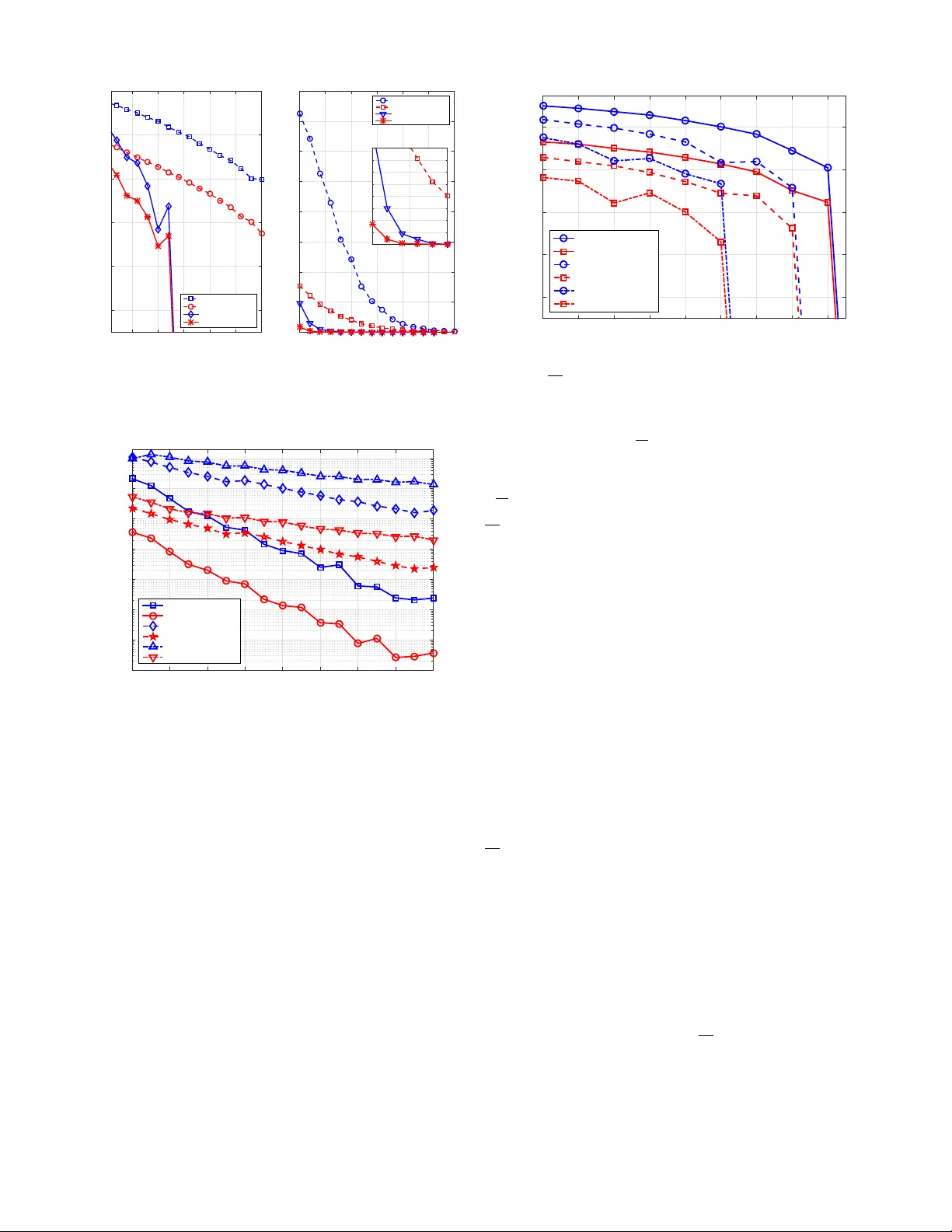
Leave a Comment