One-Shot Session Recommendation Systems with Combinatorial Items

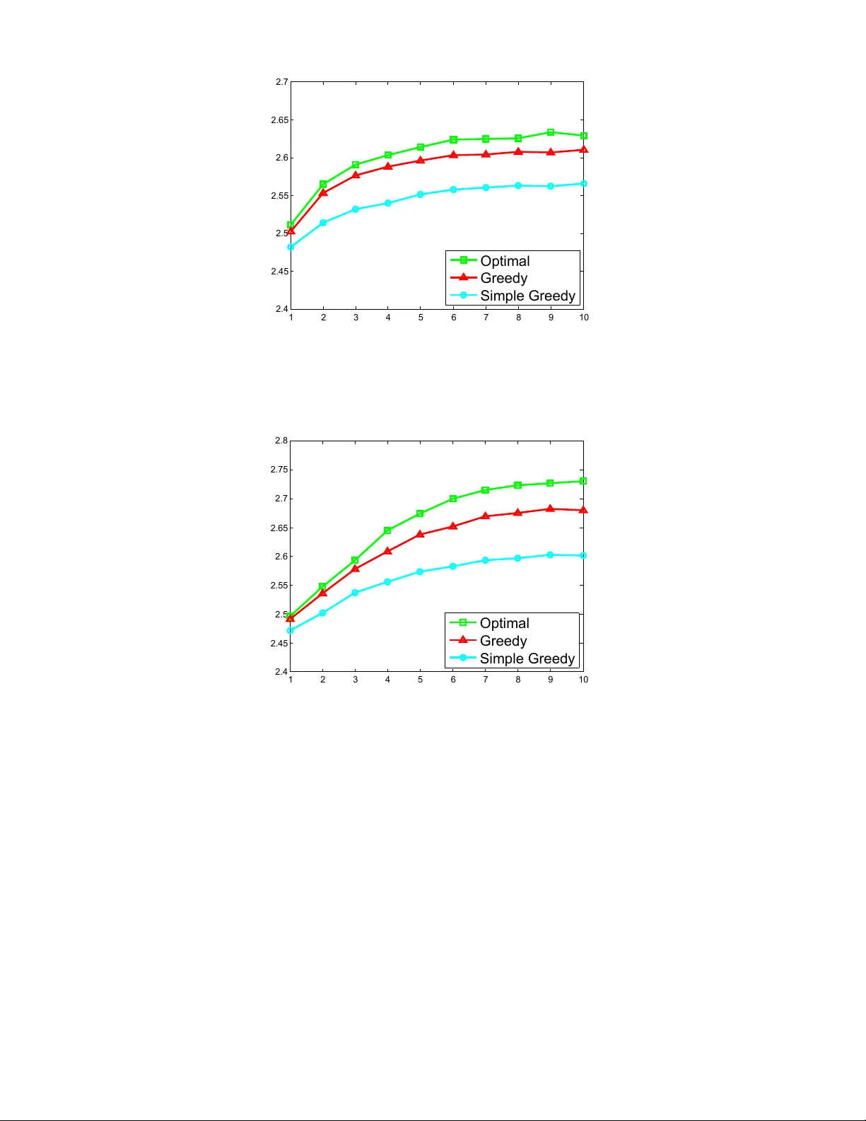
One-Shot Session Recommendation Systems with Combinatorial Items Y ahel Da vid Dotan Di Castro Zohar Kar nin Abstract In recent years, content recommendation systems in large websites (or content pr ovider s ) capture an increased focus. While the type of content varies, e.g. movies, articles, mu- sic, adv ertisements, etc., the high level problem remains the same. Based on knowledge obtained so far on the user, rec- ommend the most desired content. In this paper we present a method to handle the well known user-cold-start problem in recommendation systems. In this scenario, a recommen- dation system encounters a ne w user and the objecti ve is to present items as relev ant as possible with the hope of keep- ing the user’ s session as long as possible. W e formulate an optimization problem aimed to maximize the length of this initial session, as this is believed to be the key to hav e the user come back and perhaps register to the system. In partic- ular , our model captures the fact that a single round with low quality recommendation is likely to terminate the session. In such a case, we do not proceed to the ne xt round as the user leav es the system, possibly never to seen again. W e denote this phenomenon a One-Shot Session . Our optimization prob- lem is formulated as an MDP where the action space is of a combinatorial nature as we recommend in each round, mul- tiple items. This huge action space presents a computational challenge making the straightforward solution intractable. W e analyze the structure of the MDP to prov e monotone and sub- modular like properties that allo w a computationally efficient solution via a method denoted by Gr eedy V alue Iter ation (G- VI). 1 Introduction In the user cold-start problem a new user is introduced to a recommendation system. Here, the system often has little to no information about this new user and must provide rea- sonable recommendation nonetheless. A good recommen- dation system must on one hand provide quality (initially based on item popularity) recommendations to such users in order to keep them engaged, and on the other hand learn the new users’ personal preferences as quickly as possible. The initial session of a user with a recommendation system is critical as in it, the user decides whether to terminate the session, and possibly ne ver return, as opposed to re gistering to the site or becoming a regular visitor of the system. W e refer to this phenomenon as that of a one-shot session . This Copyright c  2015, Association for the Advancement of Artificial Intelligence (www .aaai.org). All rights reserv ed. brings emphasis on the need to obtain guarantees not only for a long horizon but also for a v ery short one. The one-shot session framework leads to a highly natural objectiv e: Maximize the session length, i.e. the number of items consumed by the user until terminating the session. Indeed, the longer the user engages with the system the more likely she is to register and become a regular user . Our focus is on recommendation systems in which we present multiple items in each round. The user will either choose a single item and proceed to the next round, or choose to terminate the session. The property of having multiple items allo ws us to learn about the user’ s preferences based on the items chosen, versus those that were skipped. A typical session length is quite short as it consists of a handful of rounds. This translates to us ha ving v ery fe w data to learn from in order to personalize our recommendations. Due to the limited amount of information we are forced to restrict ourselves to a very simple model. For this reason we take a similar approach to that in (Agrawal, T enek et- zis, and Anantharam 1989; Salomon and Audibert 2011; Maillard and Mannor 2014) and assume that each user be- longs to one of a fixed number of M user types (in the mentioned works these were called user clusters), such as man/woman, low/high income, or latent types based on previously observed sessions. The simplicity of the model translates into M being a small integer . W e assume that the model associated with each of the M user types is known 1 . That is, for any k -tuple of items, the probability of each of the items to be chosen, and the probability of the session ter - minating given the user type is known. W e emphasize the fact that a complete recommendation system will start with the simple model with M being a small constant, and for users that are ‘hooked’, i.e. remain for a long period / regis- ter , we may mo ve to a more complex model where for exam- ple a user is represented by a high dimensional vector . W e do not discuss the latter more complex system, aimed for users with a long history , as it is outside the scope of our paper . The problem we face can be formulated as a Markov Decision Problem (MPD; (Bertsekas and Tsitsiklis 1995; Sutton and Barto 1998)). In each round the state is a dis- 1 Learning the correct model for a user type can be done for example from data collected from different users whose identity is known. In either case this can be handled independently hence we do not deal with this issue tribution over [ M ] reflecting our kno wledge about the user . W e choose an action consisting of k different items from the item set L . The user either terminates the session, leading to the end of the game or chooses an item, moving us to a dif- ferent state as we gained some knowledge as to her identity . Notice that any av ailable context , e.g. time of day , gender , or basic information av ailable to us can be used in order to set the initial state. The formulated MDP can be solved in order to obtain the optimal strategy; the computational cost scales as the size of the action space and the state space. Since M is restricted to be small, the size of the state space does not present a real challenge. Ho wev er , the action space has a size of | L | k which is typically huge. The number of av ailable items can be in the hundreds if not thousands and a system presenting ev en a handful of items will have for the v ery least billions of possible actions. For this reason we seek a solution that scales relati vely to k | L | rather than | L | k . T o this end we require an additional mild assumption, that can be viewed as a quantitive extension of the irrele vant al- ternatives axiom (see Section 4). W ith this assumption we are able to provide a solution (Section 5) based on a greedy approach that scales as k | L | and has a constant competitive ratio with the computationally unbounded counterpart. The main component of the proof is an analysis showing that the sub-modularity and monotonicity of the immediate re war d in a r ound translates into monotone and sub-modular-like properties of the so called Q -function in a modified v alue it- eration procedure we denote by Gr eedy V alue Iter ations (G- VI). Giv en these properties we are able to show , via an easy adaptation of the tools provided in (Nemhauser , W olsey , and Fisher 1978) for dealing with submodular monotone func- tions, that the greedy approach emits a constant approxima- tion guarantee. W e emphasize that in general, a monotone submodular rew ard function does not in any way translate into a monotone submodular Q function, and we exploit spe- cific properties of our model in order to prov e our results; to demonstrate this we sho w in Appendix G an example for a monotone submodular immediate rew ard function with a corresponding Q function that is neither monotone nor sub- modular . W e complement the theoretical guarantees of our solution in Section 6 with experimental results on synthetic data showing that in practice, our algorithm has performance almost identical to that of the computationally unbounded algorithm. 2 Related W ork Many pre vious papers provide adapti ve algorithms for man- aging a recommendation system, yet to the best of our knowledge, non of them deal with one-shot sessions. The tools used include Multi-armed Bandits (Radlinski, Klein- berg, and Joachims 2008), Multi-armed bandits with sub- modularity , (Y ue and Guestrin 2011), MDPs (Shani, Heck- erman, and Brafman 2005), and more. A common property shared by these results is the assumption of an infinite hori- zon. Specifically , a poor recommendation given in one round cannot cause the termination of the session, as in one-shot sessions, b ut only result in a small re ward in the same single round. This crucial difference in the ‘cost’ of a single bad round in the setups of these papers versus ours is very lik ely to cause these methods to f ail in our setup. A paper that par - tially a voids this drawback is by (Deshpande and Montanari 2012), where other than a guarantee for an infinite horizon the authors provide a multiplicativ e approximation to the op- timal strategy at all times. A notable difference between our setup is the fact that the recommendations there consist of a single item rather than multiple items as required here. This, along with the somewhat vague connection to our one-shot session setup exclude their methods from being a possible solution to our problem. Our work can be casted as a Partially Observ able MDP (POMDP; (Kaelbling, Littman, and Cassandra 1998)), where the agent only has partial (sometimes stochastic) knowledge o ver the current state. Our problem stated as a POMDP instance admits M + 1 states, one for each user type and an additional state reflecting the session end. The bene- fit of such an approach is the ability to significantly reduce the size of the state space, from exp( M ) potentially do wn to M + 1 . Nev ertheless, we did not chose this approach as the gain is rather insignificant due to M being a small con- stant, while the inherent complication to the analysis and al- gorithm make it difficult to deal with the large action space, forming the main challenge in our setting. Recently , (Sat- sangi, Whiteson, and Oliehoek 2015) presented a result deal- ing with a combinatorial action space in a POMDP frame- work, when designing a dynamic sensor selection algorithm. They analyze a specific reward function that is af fected only by the lev el of uncertainty of the current state, thereby push- ing to wards a v ariant of pure exploration. The specific prop- erties of their reward function and MDP translate into a monotone and submodular Q -function. These properties are not present in our setup, in particular due to the fact that a session may terminate, hence the methods cannot be ap- plied. Furthermore, our greedy VI variant is slightly more complex than the counterpart in (Satsangi, Whiteson, and Oliehoek 2015) as it is tailored to ensure the (approximate) monotonicity of Q ; this is an issue that was not encountered in the problem setup of (Satsangi, Whiteson, and Oliehoek 2015). Another area which is related to our w ork is that of “Com- binatorial Multi Armed Bandits” setup (C-MAB; see (Chen, W ang, and Y uan 2013) and references within). Here, sim- ilarly to our setup, in each round the set of actions av ail- able to us can be described as subsets of a set of options (denoted by arms in the C-MAB literature). These methods cannot directly be applied to our setting due to the infinite horizon property mentioned above. Furthermore, the meth- ods given there that help deal with the combinatorial nature of the problem cannot be applied in our setting since the majority of our efforts lie in characterizing properties of the Q -function; an object that has no meaning in MAB settings but only in MDPs. 3 Problem F ormulation In this section we provide the formal definition of our prob- lem. W e first provide the definition of a Markov Decision Process (MDP). W e continue to describe our setup and its different notations, and then formulate it as an MDP . Marko v Decision Processes An MDP is defined by a tuple h X , U , P, R i where X is a state space, U is a set of actions, P is a mapping from state-action pairs to a probability distrib ution over the next-states, and R is a mapping from the state-action-next-state to the rew ard. The MDP defines a process of rounds. In each round t we are at a state c ∈ X and must choose an action from U. Ac- cording to our action, the following state and the reward r t are determined according to P, R . The objectiv e of an MDP is to maximize the cumulativ e sum of rew ards with a future discount of γ < 1 , i.e. P ∞ t =0 γ t R ( c t , w t ) , where w t is the action taken at time t , c t is the state at time t , and R ( c t , w t ) is the expected re ward giv en the action-state pair . For this objectiv e we seek a policy π mapping each state to an ac- tion. The objecti ve of planing in an MDP is to find a policy π maximizing the value function V π ( c ) , E " ∞ X t =0 γ t R  c t , π  c t       c 0 = c , π # , where the value of V π ( c ) is the long-term accumulated re- ward obtained by following the policy π , starting in state c . W e denote the optimal v alue function by V ∗ ( c ) = sup π V π ( c ) . A policy π ∗ is optimal if its corresponding value function is V ∗ (see (Bertsekas and Tsitsiklis 1995) for details). The Bellman’ s oper ator (or DP operator ) maps a function V : X → R + (where R + is the set of non-negati ve reals) to another function ( T V ) : X → R + and is defined as follo ws. ( T V )( c ) = max w ∈ U X c 0 ( R ( c , w , c 0 ) + γ V ( c 0 )) P ( c 0 | c , w ) , (1) where c and c 0 denote the current and next state, respec- tiv ely . Under mild conditions, the equation V ( c ) = ( T V )( c ) is known to have a unique solution which is the fixed point of the equation and equals to V ∗ . A known method for finding V ∗ is the V alue Iteration (VI; (Bertsekas and Tsitsiklis 1995; Sutton and Barto 1998)) algorithm which is defined by ap- plying The DP operator (1) repeatedly on an initial function V 0 (e.g. the constant function mapping all states to zero). More precisely , applying (1) t times on V 0 yields V t , T t V 0 and the VI method consists of estimating lim t →∞ V t . The VI algorithm is known to conv erge to V ∗ ( c ) . How- ev er, computational dif ficulties arise for large state and ac- tion spaces. Notations Let us first formally define the rounds of the user-system interaction and our objecti ve. When a new user arrives to the system (e.g., content provider) we begin a session . At each round, we present the user a subset of up to k items from the set of av ailable items L . The user either terminates the session, in which case the session ends, or chooses a single item from the set, in which case we continue to the next round. The reward is either r = 1 if the user chose an item 2 or r = 0 otherwise. Follo wing a common framework for MDPs, our objectiv e is to maximize the sum of re wards with future rewards discounted by a factor of γ . That is, by denoting r t the re ward of round t and T the random v ariable (or random time) describing the total number of rounds, we aim to maximize E " T − 1 X t =0 γ t r t # . (2) The reason for considering γ < 1 is the fact that the dif- ference between a session of say length 10 and length 5 is not the same as that of length 6 and 1. Indeed in the user cold-start problem one can think of a model where ev ery ad- ditional item observed by the user increases the probability of her registering, yet this function is not linear but rather monotone increasing and concav e. W e continue to describe the modeling of users. Recall that users are assumed to characterized by one of the members of the set [ M ] . Our input contains for e very set w ⊆ L of items, e very user type m ∈ [ M ] , and any item ` ∈ w the probability p ( ` | m, w ) of the user of type m choosing item ` when presented the set w . In the session dynamics described abov e we maintain at all times a belief regarding the user type, denoted by 3 c ∈ ∆ M , with ∆ M being the set of dis- tributions over [ M ] . Notice that giv en the distribution c we may compute for e very set w and item ` ∈ w the probability of the user choosing item ` . W e denote this probability by p ( ` | c , w ) = X m ∈ [ M ] c ( m ) · p ( ` | m, w ) Assume now that at round t , our belief state is c t = c , we presented the user a set of items w , and the user chose item ` . The following observation provides the posterior probability c t +1 also denoted by c 0 `,w, c . The proof is based on the Bayes rule; as it is quite simple we defer it to Appendix A in the supplementary material. Observation 1 The vector c 0 `,w, c is the posterior type- pr obability for a prior c , action w and a chosen item ` . This pr obability is obtained by c 0 `,w, c ( m 0 ) = p ( ` | m 0 , w ) c ( m 0 ) p ( ` | c , w ) . (3) F ormulating the Problem as an MDP W e formulate our problem as an MDP as follows. The state space X is defined as ∆ M ∪ { c ∅ } where c ∅ denotes the ter- mination state. The action space U consists of all subsets w ⊆ L of cardinality | w | ≤ k . The re ward function R de- pends only on the target state and is defined as 1 for any c ∈ ∆ M and zero for c ∅ . As a result of Observ ation 1, we are able to define the transition function P : P ( c 0 | c , w ) =    X ` ∈ L ( c 0 , c ,w ) p ( ` | c , w ) L ( c 0 , c , w ) 6 = ∅ 0 L ( c 0 , c , w ) = ∅ , 2 It is an easy task to extend our results to a setting where dif fer- ent items incur different rewards. For simplicity howe ver we keep it simple and assume equality between items, in terms of rew ards. 3 Eventually we consider a discretization of the simplex, but for clarity we discuss this issue only at a later stage. where the set L ( c 0 , c , w ) is defined as  `     ∀ m 0 , c 0 ( m 0 ) = p ( ` | m 0 , w ) c ( m 0 ) P m ∈ M p ( ` | m, w ) c ( m ))  that is the set containing ` ∈ L such that (3) is satis- fied. The final missing definition to the transition function is the probability to move to the termination state, denoted by c ∅ , defining the session end. For it, P ( c ∅ | c , w ) = 1 − P ` ∈ w p ( ` | c , w ) . 4 User Modeling Assumptions In order to obtain our theoretical guarantees we use assump- tions regarding the user behavior . Specifically , we assume a certain structure in the function mapping a item set w and a item ` ∈ w to the probability that a user of type m (any m ) will choose the item ` when presented with the item set w . T o assess the validity of the belo w assumption consider an example standard model 4 where each item ` in w (and the empty item) has a positi ve v alue µ ` for the user and the cho- sen item is drawn with probability proportional to µ ` . W e note that the below assumptions hold for this model. The first assumption essentially states that at all states there is a constant, bounded away from zero, probability to reach the termination state. In our setup this translates into an assumption that ev en gi ven kno wledge of the user type, the probability of the user ending the session remains non- zero. Needless to say this is a highly practical assumption. Assumption 1 F or a constant B > 1 , any set of content items w ∈ L i wher e i ≤ k , any types vector c ∈ ∆ M and a content item ` ∈ L , it holds that X ` ∈ L p ( ` | c , w ) ≤ 1 B . In what follows, our approximation guarantee will depend on B , that is on ho w much the best-case-scenario probability of ending a session is bounded away from zero. The second assumption assert independence between the probabilities of choosing different content items. Assumption 2 F or every m ∈ M , a set of content items w and a content item ` 0 6∈ w it holds that p ( ` | m, w ) = p ( ` | m, w ∪ ` 0 ) + p ( ` 0 | m, w ∪ ` 0 ) p ( ` | m, w ) . (4) The above assumption is related to the independence of irr elevant alternatives axiom (IIA) (Saari 2001) of decision theory , stating that “If A is preferred to B out of the choice set { A, B } , introducing a third option X , expanding the choice set to { A, B , X } , must not make B preferable to A ”. Our assumption is simply a quantitiv e version of the abov e. 5 A pproximation Of the V alue Function In this section we develop a computationally efficient ap- proximation of the value function for the setup described abov e. W e begin with dealing with the action space, and later we also take into consideration the continuity of the state space. 4 An example for where this modeling is implicitly made is in the setting of a Multinomial Logistic Re gression . Addressing the Lar geness of the Action Space by Sub-modularity In this section we provide a greedy approach dealing with the large action space, leading to a running time scaling as O ( k | L | + | X | ) . For clarity we ignore the fact that X is infi- nite and defer its discretization to the Section 5. The outline of the section is as follows: W e first mention that the im- mediate rew ard function, when viewed as a function of the action, is monotone and submodular . Next, we define a mod- ified value-iteration procedure we denote by gr eedy value it- eration (G-VI), resulting in a sequence of approximate value function V t and Q -functions Q t , obtained in the iterations of the procedure. W e show that these Q t functions are approx- imately monotone and approximately submodular and that for functions with these approximate monotone-submodular properties, the greedy approach provides a constant approx- imation for maximization; we are not aware of papers us- ing the e xact same definitions for approximate monotonicity and submodularity yet we do not consider this contribution as major since the proofs regarding the greedy approach are straightforward gi ven existing literature. Finally , we tie the results together and obtain an approximation of the true Q function, as required. Since it is mainly technical and due to space limitations, we defer the proof that the rew ard function is monotone and submodular to Appendix B. W e now turn to describe the pro- cess G-VI. W e start by defining our approximate maximum operator Definition 2 Let L be a set, f : L → R , and let 0 ≤ k ≤ | L | be an inte ger . W e denote by L k the set of subsets of L of size k . The oper ators g max , arg g max (the super script “g” for gr eedy) are defined as follows g max w ∈ L 0 f ( w ) = f ( ∅ ) , arg g max w ∈ L 0 f ( w ) = ∅ , g max w ∈ L k +1 f ( w ) = max ` ∈ L f (arg g max w 0 ∈ L k f ( w 0 ) ∪ { ` } ) , arg g max w ∈ L k +1 f ( w ) = arg g max w ∈ L k f ( w ) ∪ arg max ` ∈ L f  arg g max w ∈ L k f ( w ) ∪ { ` }  . Informally , the g max operator maximizes the v alue of a func- tion f ov er subsets of restricted size by greedily adding el- ements to a subset in a way that maximizes f . For a v alue function V we define the Q function as Q V ( w 0 , c ) = X ` ∈ L p ( ` | c , w 0 )(1 + γ V ( c 0 `,w 0 , c )) (5) When it is clear from context which V is referred to, we omit the subscript of it. Recall that the standard DP opera- tor is defined as ( T V ) ( c ) = max w ∈ L k Q ( w , c ) . Using our greedy-based approximate max we define two greedy-based approximate DP operator . The first is denoted as the simple- greedy approach where ( T simple greedy V )( c ) = g max w Q ( w , c ) (6) As it turns out, the simple-greedy approach does not nec- essarily conv erge to a quality value function. In particu- lar , the Q function obtained by it does not emit necessary monotone-submodular-lik e qualities that we require for our analysis. W e hence define the second DP operator we call the greedy operator . Definition 3 F or a function V : X → R + we define ( T gr eedy V ) ( c ) = max w ∈ G Q V ( w , c ) (7) wher e the set G is defined in the following statement, G = { w |∃ c ∈ X s.t w = arg g max w 0 ∈ L k Q ( w 0 , c ) } , In words, we take advantage of the fact that the number of states is small (as opposed to the number of actions) and use the g max operator not to associate actions with states but rather to reduce the number of actions to be at most the same as the number of states. W e then choose the actual arg max for each state, from the small subset of actions. No- tice that the compositional complexity of the T greedy opera- tor is O ( k | L | + | X | ) , as opposed to O ( k | L | ) as the T simple greedy operator . In Appendix 6 , we explore whether there is a need for the further complication inv olved with using T greedy rather than T simple greedy , or whether its use is needed only for the analysis. W e show that in simulations, the system using the T greedy operator significantly outperforms that using the sim- pler T simple greedy operator . Recall that the value iteration (VI) procedure consists of starting with an initial value function, commonly the zero function, then performing the T operator on V multiple times until con ver gence. Our G-VI process is essentially the same, but with the T greedy operator . Specifically , we initial- ize V to be the zero function and analyze the properties of T t greedy V for t > 0 . In our analysis we manage to tie the value of T t greedy V computed w .r .t. a decay v alue γ (Equation (5)), to the v alue of T t V , the true VI procedure, computed w .r .t. a decay value of γ 0 with γ 0 ≈ 0 . 63 γ . T o dispaly our result we denote by T t γ 0 V the iterated DP operator done on V w .r .t. decay value γ 0 . The proof is giv en in Appendix C . Theorem 4 Let γ > 0 . Under Assumptions 1 and 2, for B ≥ 2 , zer o initiation of the value function (namely , V = 0 ) and for any t ≥ 1 , it is obtained that  T t gr eedy V  ( c ) ≤ ( T t V )( c ) (8) β  ( T t β γ V )( c ) − Ω t, c  ≤ ( T t gr eedy V )( c ) (9) with β = 1 − 1 /e ≈ 0 . 63 , Ω t, c , t − 1 X i =0 ( β γ ρ ( c )) i ( k − 1) θ ( c ) , ρ ( c ) , max w ∈ L k X m ∈ M c ( m ) X ` ∈ L P ( ` | m, w ) , and θ ( c ) , max ` 0 ∈ L,w ∈ L k X m ∈ M c ( m ) P ( ` 0 | m, w ∪ ` 0 ) X ` ∈ L P ( ` | m, w ) γ B − γ (10) T o better understand the meaning of the above e xpression we estimate the v alue of Ω t, c for the initial state c in reason- able settings. Specifically , we would lik e estimate λ , Ω t, c ( T t β γ V )( c ) . In cases where λ is a small constant we get a constant mul- tiplicativ e approximation of the v alue function obtained via the optimal, computationally inefficient maximization. In the supplementary material (Lemma 19) we provide the bound λ = Ω t, c ( T t β γ V )( c ) ≤ ( k − 1) ¯ θ ( c ) ρ ( c ) The proof is purely technical. Notice that ρ ( c ) is in fact the probability of the user , gi ven the state c and us choosing the best possible action, choosing a link rather than terminat- ing the session. Assuming a large number of content items (compared to k ) it is most likely that for ev ery type m ∈ M there are much more than k fav orable items. This informally means that either the probability of choosing any item ` among a set w is roughly ρ ( c ) /k or w is a poor choice of links and the probability of ending the session when present- ing w is significantly lo wer than ρ ( c ) . It is thus reasonable to assume that ( k − 1) θ ( c ) . ρ ( c ) 2 γ ( B − γ ) . Hence λ . ρ ( c ) γ ( B − γ ) ≤ γ B ( B − γ ) For example, for B = 2 and γ = 0 . 75 . Then we have λ ≤ 0 . 3 , hence 0 . 44( T t β γ V )( c ) ≤ ( T t greedy V )( c ) , meaning we get a multiplicativ e 0 . 44 approximation compared to the optimal operator with γ 0 ≈ 0 . 47 . Addressing Both The Continuity of State Space and The Largeness of the Action Space Recall that the state space of our model is continuous. As our approach requires scanning the state space we present here an analysis of our approach taken over a discretized state space. That is, rather than working ov er ∆ M (the entire M dimensional simplex) our finite state space X is taken to be an  -net, w .r .t. the L 1 -norm, ov er ∆ M . As before, the v alue iteration we suggest takes the greedy approach where the only difference is in the definition of the Q -function. Definition 5 The Q g d -function, based on a function V t − 1 g d ( c ) mapping a state to a value is defined as follows: Q t g d ( w , c ) = X ` ∈ L p ( ` | c , w )(1 + γ V t − 1 g d ( \ c 0 `,w, c )) . (11) wher e \ c 0 `,w, c is defined as the closest point in X to c 0 `,w, c . Analogically to before, we define the T g d operator ov er a value function V g d as V t g d ( c ) = ( T g d V t − 1 g d )( c ) = max w ∈ G Q g d ( w , c ) (12) with G being defined w .r .t. the finite state set X. In Ap- pendix E we prov e the following theorem, giving the analy- sis of the abov e value iteration procedure. Theorem 6 Under Assumptions 1 and 2, for B ≥ 2 , zer o initiation of the value function (namely , V = 0 ), a state space formed via an L 1  -net, and for any t ≥ 1 we have  T t g d V  ( c ) ≤ ( T t V )( c ) + O (  ) β  ( T t β γ V )( c ) − Ω t, c (1 + O (  ))  ≤ ( T t g d V )( c ) wher e β , Ω t, c ar e the same as in Theorem 4. For sufficiently small  = Ω(1) , the result is essentially the same as that in Section 5. 6 Experiments 5 In this section we in vestigate numerically the algorithms suggested in Section 5. W e examine four types of CP poli- cies: 1. Random policy , where the CP provides a (uniformly) random set of content items at each round. 2. Regular DP operator policy , namely T as in (1), in which the maximum is computed exactly . The computa- tional complexity of each iteration of the VI with the original DP operator is of order of O ( | X || L | K ) . 3. Greedy Operator policy , namely following the T g d oper- ator as in (12). In this case the computational complexity of each iteration of the G-VI is of order of O ( | X || L | K + | X | 2 ) . 4. Simple Greedy CP , namely following the T simple greedy opera- tor as in (6). No theoretical guarantees are provided for this CP , but since its computational complexity of each iteration of the VI is of order of O ( | X || L | K ) and its similarity to the gr eedy CP , we are interested in its performances. W e conducted our experiments on synthetic data. The users’ policy implemented the following model relating the scores to the users’ choice, P ( ` | m, w ) = ` m P ` 0 ∈ w ` 0 m + p m , where ` m is a score expressing the subjective value of item ` for users of type m and where p m expresses the tendency of user of a type m to terminate the session. It is easy to verify that for p m large enough compared to the scores, As- sumption 1 holds, and that Assumption 2 holds for any value assigned to ` m and p m . For the experiments, we considered the case of M = 4 , | L | = 13 , k = 3 and γ = 1 . The scores were chosen as follows: For all types, the termination score was p m = 0 . 5 . Four items were chosen i.i.d. uniformly at random from the interval [0 , 0 . 6] . The remaining 8 items where chosen such that for each user type, 2 items are uniformly distributed in [0 . 5 , 1] (strongly related to this type), while the other 6 are drawn uniformly from [0 , 0 . 5] . W e repeated the experiment 500 times, where for each repetition a dif ferent set of scores was generated and 100 , 000 sessions were generated (a total of 50 M sessions). In Figure 1 we present the av erage session length un- der the optimal, gr eedy and simple greedy CPs for differ - ent numbers of iterations ex ecuted for computing the V alue 5 Additional experiments are provided in Section F of the sup- plementary material. function. The av erage length that was achiev ed by the ran- dom CP is 1 . 3741 , much lower than that of the other meth- ods. The standard de viation is smaller that 10 − 3 in all of our measures. As shown in Figure 1, the extra comparison step in the gr eedy CP compared to the simple gr eedy CP substan- tially improv es the performance. 1 2 3 4 5 6 7 8 9 10 2.3 2.35 2.4 2.45 2.5 2.55 2.6 Optimal Greedy Simple Greedy Figure 1: A verage session length under the optimal, gr eedy and simple gr eedy ( y -axis) CPs vs. number of iterations of the related VI computation ( x -axis). The average length of the random CP is 1 . 3741 (not shown). 7 Discussion and Conclusions In this work we developed a new framew ork for analyzing recommendation systems using the MDP frame work. The main contribution is two-fold. First, we provide a model for the user-cold start problem with one-shot sessions, where a single round with lo w quality recommendations may end the session entirely . W e formulate a problem where the objec- tiv e is to maximize the session length 6 . Second, we suggest a greedy algorithm overcoming the computational hardship in volved with the combinatorial action space present in rec- ommendation system that recommend se veral item at a time. The effecti veness of our theoretical results is demonstrated with experiments on synthetic data, where we see that our method performs practically as well as the computationally unbounded one. As future work we plan to generalize our techniques for dealing with the combinatorial action space to setups other than the user-cold start problem, and aim to characterize the conditions in which the Q function is (approximately) monotone and submodular . In particular we will consider an 6 Another problem, which is somehow related to the cold-start problem, is the problem of devices that are shared between sev eral users (White et al. 2014; File 2013). In this scenario, several people share the same device while the content provider is aware only of the identity of the de vice and not of the identity of the user . This phenomenon typically occurs with devices in the same household, shared by the members of the family . The methods developed in this work can be easily adapted to solve this problem as well. extension to POMDPs as well that may deal with similar settings in which M can take larger v alues. References [Agrawal, T eneketzis, and Anantharam 1989] Agrawal, R.; T eneketzis, D.; and Anantharam, V . 1989. Asymptotically efficient adaptive allocation schemes for controlled marko v chains: Finite parameter space. Automatic Contr ol, IEEE T ransactions on 34(12):1249–1259. [Bertsekas and Tsitsiklis 1995] Bertsekas, D. P ., and Tsitsiklis, J. N. 1995. Neuro-dynamic programming: an ov erview . In De- cision and Contr ol, 1995., Pr oceedings of the 34th IEEE Con- fer ence on , volume 1, 560–564. IEEE. [Chen, W ang, and Y uan 2013] Chen, W .; W ang, Y .; and Y uan, Y . 2013. Combinatorial multi-armed bandit: General frame- work, results and applications. In Pr oceedings of the 30th Inter- national Confer ence on Mac hine Learning (ICML 13), Atlanta, Geor gia, USA . [Deshpande and Montanari 2012] Deshpande, Y ., and Monta- nari, A. 2012. Linear bandits in high dimension and recommen- dation systems. In Communication, Contr ol, and Computing (Allerton), 2012 50th Annual Allerton Confer ence on , 1750– 1754. IEEE. [File 2013] File, T . 2013. Computer and internet use in the united states. P opulation Char acteristics . [Kaelbling, Littman, and Cassandra 1998] Kaelbling, L. P .; Littman, M. L.; and Cassandra, A. R. 1998. Planning and acting in partially observable stochastic domains. Artificial intelligence 101(1):99–134. [Maillard and Mannor 2014] Maillard, O., and Mannor , S. 2014. Latent bandits. In Proceedings of the 31th International Confer ence on Machine Learning, ICML 2014, Beijing, China, 21-26 J une 2014 , 136–144. [Nemhauser , W olsey , and Fisher 1978] Nemhauser, G. L.; W olse y , L. A.; and Fisher , M. L. 1978. An analysis of approximations for maximizing submodular set functionsi. Mathematical Pr ogramming 14(1):265–294. [Radlinski, Kleinberg, and Joachims 2008] Radlinski, F .; Klein- berg, R.; and Joachims, T . 2008. Learning div erse rankings with multi-armed bandits. In Proceedings of the 25th international confer ence on Machine learning , 784–791. A CM. [Saari 2001] Saari, D. 2001. Decisions and elections: explain- ing the unexpected . Cambridge University Press. [Salomon and Audibert 2011] Salomon, A., and Audibert, J.-Y . 2011. Deviations of stochastic bandit regret. In Algorithmic Learning Theory , 159–173. Springer . [Satsangi, Whiteson, and Oliehoek 2015] Satsangi, Y .; White- son, S.; and Oliehoek, F . A. 2015. Exploiting submodular value functions for faster dynamic sensor selection. In AAAI 2015: Pr oceedings of the T wenty-Ninth AAAI Conference on Artificial Intelligence . [Shani, Heckerman, and Brafman 2005] Shani, G.; Heckerman, D.; and Brafman, R. I. 2005. An mdp-based recommender system. In J ournal of Machine Learning Researc h , 1265–1295. [Sutton and Barto 1998] Sutton, R. S., and Barto, A. G. 1998. Intr oduction to reinfor cement learning . MIT Press. [White et al. 2014] White, R. W .; Hassan, A.; Singla, A.; and Horvitz, E. 2014. From de vices to people: Attribution of search activity in multi-user settings. In Pr oceedings of the 23r d inter - national confer ence on W orld wide web , 431–442. International W orld W ide W eb Conferences Steering Committee. [Y ue and Guestrin 2011] Y ue, Y ., and Guestrin, C. 2011. Linear submodular bandits and their application to di versified retrie val. In Advances in Neural Information Pr ocessing Systems , 2483– 2491. A Missing Proofs Proof of Lemma 1 Here we use c 0 as a short for c 0 `,w,C . By Bayes’ theorem, for any c , w ∈ L k and ` ∈ L , it follows that c 0 ( m 0 ) = P ( c ( m 0 ) = 1 | `, w, c ) = P ( c ( m 0 ) = 1 , ` | w, c ) P ( ` | w , c ) = P ( ` | c ( m 0 ) = 1 , w, c ) P ( c ( m 0 ) = 1 | w, c ) P ( ` | w , c ) = p ( ` | m 0 , w ) c ( m 0 ) P m ∈ M p ( ` | m, w ) c ( m ) , (13) where P ( c ( m 0 ) = 1) stands for the probability that the user type is m 0 . So, the result is obtained.  B Additional Propositions and Lemmas In the following propositions and lemmas we deri ve some results related to greedy maximization of submodular functions. These results are used for the proofs of Theorems 4 and 6. Model Properties In the following proposition we sho w the monotonicity and submodularity properties of the chosen model. Proposition 7 Under Assumption 2, for any two sets of content items w b ⊃ w a and a content item ` 0 6∈ w b , it holds that ( monotonicity ) X ` ∈ L p ( ` | m, { w b ∪ ` 0 } ) − X ` ∈ L p ( ` | m, w b ) ! ≥ 0 , (14) and ( submodularity ) X ` ∈ L p ( ` | m, { w a ∪ ` 0 } ) − X ` ∈ L p ( ` | m, w a ) ! ≥ X ` ∈ L p ( ` | m, { w b ∪ ` 0 } ) − X ` ∈ L p ( ` | m, w b ) ! , (15) for any type m ∈ M . Proof: By Equation (4) it follo ws that X ` ∈ L p ( ` | m, { w b ∪ ` 0 } ) − X ` ∈ L p ( ` | m, w b ) ! = p ( ` 0 | m, { w b ∪ ` 0 } ) 1 − X ` ∈ L p ( ` | m, w b ) ! ≥ 0 . (16) So, Equation (14) is obtained. For pro ving Equation (15), we note that X ` ∈ L p ( ` | m, { w a ∪ ` 0 } ) − X ` ∈ L p ( ` | m, w a ) ! = p ( ` 0 | m, { w a ∪ ` 0 } ) 1 − X ` ∈ L p ( ` | m, w a ) ! ≥ 0 . (17) Then, since by Equation (4) we hav e that p ( ` 0 | m, { w a ∪ ` 0 } ) ≥ p ( ` 0 | m, { w b ∪ ` 0 } ) , and that X ` ∈ L p ( ` | m, w b ) ≥ X ` ∈ L p ( ` | m, w a ) . Equation (15) is obtained by Equations (16) and (17).  Almost Submodular Maximization In this Section we provide three Lemmas: Lemma 8 is the main result which generalizes the classical result proposed in (Nemhauser, W olse y , and Fisher 1978) to ”almost”-monotone and ”almost”-submodular functions. Lemma 8 Let g : 2 L → R + be a function mapping subsets of L to non-negative r eals with the following pr operties: 1. g ( ∅ ) = 0 2. for all w ⊂ L, ` ∈ L , g ( w ∪ ` ) ≥ g ( w ) −  3. for all w a ⊆ w b ⊆ L and ` ∈ L , g ( w a ∪ ` ) − g ( w a ) ≥ g ( w a ∪ ` ) − g ( w a ) − θ for some scalar θ . Then, it is obtained that g ( w k ) ≥ β  max w ∈ L k g ( w ) − ( k − 1) θ − k   , wher e w k ∈ L k is obtained by the Gr eedy Algorithm and β = 1 −  1 − 1 k  k +1 ≥ 1 − 1 e (18) Proof: (Based on Nemhauser et al. 1978) By Lemma 10, for i + 1 = k we have g ( w k ) ≥  1 −  1 − 1 k  k  ( g ( OP T ) − θ ( k − 1) − k  ) , where w k is the set that obtained by the greedy Algorithm after k iterations and the set O P T attains the optimal value, namely , { O P T } = arg max w ∈ L k g ( w ) .  In the following Lemma we bound the loss of adding greedily one item to a given set. This lemma is used for the proof of Lemma 10 (which is used for the proof of Lemma 8). Lemma 9 Under the conditions of Lemma 8, after applying the Gr eedy Algorithm, it holds that g ( w i +1 ) − g ( w i ) ≥ 1 k ( g ( OP T ) − g ( w i )) − θ ( k − 1) k −  , wher e the set O P T attains the optimal value, namely , { O P T } = arg max w ∈ L k g ( w ) , and the set w i is the set that obtained by the gr eedy Algorithm after i iterations. Proof: F or every set of content items T = { ` 1 , ..., ` | T | } and j ≤ | T | , we denote T j = { ` 1 , ..., ` j } and T 0 = ∅ . So, we hav e, g ( w i ∪ T ) − g ( w i ) = | T | X j =1 g ( w i ∪ T j ) − g ( w i ∪ T j − 1 ) . Then, since for ev ery j ≥ 2 and ` ∈ L g ( w i +1 ) − g ( w i ) ≥ g ( w i ∪ ` ) − g ( w i ) , and g ( w i +1 ) − g ( w i ) ≥ g ( w i ∪ T j − 1 ∪ ` ) − g ( w i ∪ T j − 1 ) − θ , it is obtained that | T | ( g ( w i +1 ) − g ( w i )) ≥ g ( w i ∪ T ) − g ( w i ) − ( | T | − 1) θ . Therefore, g ( w i +1 ) − g ( w i ) ≥ g ( w i ∪ T ) − g ( w i ) − ( | T | − 1) θ | T | , Φ ∆ . Then, for the choice of T = O P T \ w i , since | T | ≤ k , we hav e Φ ∆ ≥ g ( w i ∪ T ) − g ( w i ) k − θ ( k − 1) k −  = g ( OP T ) − g ( w i ) k − θ ( k − 1) k −  .  In the following Lemma we bound the loss that is incurred by adding greedily a certain number of items to a set. This lemma is used for the proof of Lemma 8. Lemma 10 Under the Gr eedy Algorithm, it holds that g ( w i +1 ) ≥  1 −  1 − 1 k  i +1  ( g ( OP T ) − θ ( k − 1) − k  ) , wher e the set O P T attains the optimal value, namely , { O P T } = arg max w ∈ L k g ( w ) , and the set w i is the set that obtained by the gr eedy Algorithm after i iterations. Proof: W e prove this claim by induction over i . Since we assume that g ( ∅ ) = 0 , the base case, for i = 0 can be derived from Lemma 9. For i > 0 , it is obtained by Lemma 9 that g ( w i +1 ) ≥ 1 k g ( OP T ) − θ ( k − 1) k −  + k − 1 k g ( w i ) , Υ . Then, by the induction assumption, Υ ≥ 1 k g ( OP T ) − θ ( k − 1) k −  + k − 1 k  1 −  1 − 1 k  i  ( g ( OP T ) − θ ( k − 1) − k  ) =  1 −  1 − 1 k  i +1  ( g ( OP T ) − θ ( k − 1) − k  ) .  C Proof of Theor em 4 In this Section we provide the proof of Theorem 4. Here, we use V t ( c ) and Q t ( w, c ) for shorthand of  T greedy  t V ( c ) and Q V t − 1 ( w, c ) , respectiv ely . W e begin with a Lemma that upper bounds the value function obtained by the T greedy operator . Then, in Lemmas 12 and 13 we sho w a monotonic increasing property of the v alue function. In Lemmas 14 and 15 we sho w the con ve xity of the value function. In Lemma 16 we show the “almost”- submodularity of the Q-function, while in Lemma 17 we show the monotonicity of the Q- function. Lemma 18 shows the direct relation between a larger set of items larger long term cumulative reward. W e conclude this section with the proof of Theorem 4 which is based on Lemmas 11-18. Lemma 11 F or every c ∈ X, t ≥ 0 and zer o initiation of the value function (namely , V 0 greedy = 0 ), it holds that V t greedy ( c ) ≤ 1 B − γ . Proof: It is obtained easily by Assumption 1, that for e very c ∈ X it holds that V t greedy ( c ) ≤ 1 B  1 + γ V t − 1 greedy  , where V greedy is an upper bound on V greedy ( c ) for e very c ∈ X. So, since V 0 greedy = 0 , we hav e that V t greedy ( c ) ≤ 1 B − γ .  In the next two lemmas we sho w a monotonic increasing property of the value function that is obtained by the operator T greedy . Lemma 12 Let c 1 , c 2 ∈ X and let A 1 and B 2 be a pair of positive constants. Assume that A 1 c 1 ( m ) ≥ B 2 c 2 ( m ) , (19) for all m ∈ M . Then it holds that A 1 V 0 greedy ( c 1 ) ≥ B 2 V 0 greedy ( c 2 ) . Proof: The result is immediate since V 0 greedy ( c ) = 0 for e very c ∈ X.  Lemma 13 Let c 1 , c 2 ∈ X and let A 1 and B 2 be a pair of positive constants. Assume that A 1 c 1 ( m ) ≥ B 2 c 2 ( m ) , (20) for all m ∈ M . Then, we have for any positive inte ger t A 1 V t greedy ( c 1 ) ≥ B 2 V t greedy ( c 2 ) . Proof: W e prove the claim by induction ov er t . The base case for t = 0 holds due to Lemma 12. Assume that the lemma is satisfied for t − 1 . Recall Equation (3) characterizing c 0 `,w, c ( m 0 ) c 0 `,w, c ( m 0 ) = c ( m 0 ) p ( ` | m 0 , w ) P m ∈ M c ( m ) p ( ` | m, w ) . By plugging in with Equation (20) we get that A 1 X m ∈ M c 1 ( m ) p ( ` | m, w ) ! c 0 `,w, c 1 ( m 0 ) ≥ B 2 X m ∈ M c 2 ( m ) p ( ` | m, w ) ! c 0 `,w, c 2 ( m 0 ) , for any w ∈ L k , ` ∈ L and m 0 ∈ M , as p ( ` | m 0 , w ) ≥ 0 . Therefore, by the induction assumption applied for A 0 1 = A 1 X m ∈ M c 1 ( m ) p ( ` | m, w ) ! , B 0 2 = B 2 X m ∈ M c 2 ( m ) p ( ` | m, w ) ! , A 1 X m ∈ M c 1 ( m ) p ( ` | m, w ) V t − 1 greedy  c 0 `,w, c 1  ≥ B 2 X m ∈ M c 2 ( m ) p ( ` | m, w ) V t − 1 greedy  c 0 `,w, c 2  , (21) for ev ery ` ∈ L and w ∈ L k . Furthermore, by Equation (20) A 1 X m ∈ M c 1 ( m ) p ( ` | m, w ) ≥ B 2 X m ∈ M c 2 ( m ) p ( ` | m, w ) , (22) for ev ery ` ∈ L and w ∈ L k . So, by the fact that A 1 Q t greedy ( w, c 1 ) = A 1 X m ∈ M X ` ∈ L c 1 ( m ) p ( ` | m, w )  1 + γ V t − 1 greedy  c 0 `,w, c 1   , and also respectiv ely for B 2 and c 2 , it is obtained by Equations (21) and (22) that A 1 Q t greedy ( w, c 1 ) ≥ B 2 Q t greedy ( w, c 2 ) , (23) for any w ∈ L k . So, by Definition 3 the result is obtained.  In the following tw o lemmas we show a con vexity property of the v alue function that is obtained by the T greedy operator . Lemma 14 Let c , c 1 , c 2 ∈ X and let A , B 1 and B 2 be a tuple of positive constants. Assume that A c ( m ) = B 1 c 1 ( m ) + B 2 c 2 ( m ) , (24) for all m ∈ M . Then it holds that AV 0 greedy ( c ) ≤ B 1 V 0 greedy ( c 1 ) + B 2 V 0 greedy ( c 2 ) . Proof: T rue for initiate value function V 0 greedy ( c ) = 0 for e very c ∈ X.  Lemma 15 (Con vexity) Let c , c 1 , c 2 ∈ X and let A , B 1 and B 2 be a tuple of positive constants. Assume that A c ( m ) = B 1 c 1 ( m ) + B 2 c 2 ( m ) , (25) for all m ∈ M . W e have that for any positive inte ger t it holds that AV t greedy ( c ) ≤ B 1 V t greedy ( c 1 ) + B 2 V t greedy ( c 2 ) . Proof: W e prove the claim by induction ov er t . The base case for t = 0 holds due to Lemma 14. Assume that the lemma is satisfied for t − 1 . Recall Equation (3) characterizing c 0 `,w, c ( m 0 ) c 0 `,w, c ( m 0 ) = c ( m 0 ) p ( ` | m 0 , w ) P m ∈ M c ( m ) p ( ` | m, w ) . By plugging in with Equation (25) we get that A X m ∈ M c ( m ) p ( ` | m, w ) ! c 0 `,w, c ( m 0 ) = B 1 X m ∈ M c 1 ( m ) p ( ` | m, w ) ! c 0 `,w, c 1 ( m 0 ) + B 2 X m ∈ M c 2 ( m ) p ( ` | m, w ) ! c 0 `,w, c 2 ( m 0 ) , for any w ∈ L k , ` ∈ L and m 0 ∈ M , as p ( ` | m 0 , w ) ≥ 0 . Therefore, by the induction assumption applied for A 0 = A X m ∈ M c ( m ) p ( ` | m, w ) ! , B 0 1 = B 1 X m ∈ M c 1 ( m ) p ( ` | m, w ) ! , B 0 2 = B 2 X m ∈ M c 2 ( m ) p ( ` | m, w ) ! , A X m ∈ M c ( m ) p ( ` | m, w ) V t − 1 greedy  c 0 `,w, c  ≤ B 1 X m ∈ M c 1 ( m ) p ( ` | m, w ) V t − 1 greedy  c 0 `,w, c 1  + B 2 X m ∈ M c 2 ( m ) p ( ` | m, w ) V t − 1 greedy  c 0 `,w, c 2  , (26) for ev ery ` ∈ L and w ∈ L k . Furthermore, by Equation (25) A X m ∈ M c ( m ) p ( ` | m, w ) = B 1 X m ∈ M c 1 ( m ) p ( ` | m, w ) + B 2 X m ∈ M c 2 ( m ) p ( ` | m, w ) , (27) for ev ery ` ∈ L and w ∈ L k . So, by the fact that AQ t greedy ( w, c ) = A X m ∈ M X ` ∈ L c ( m ) p ( ` | m, w )  1 + γ V t − 1 greedy  c 0 `,w, c   , and also respectiv ely for B 1 , c 1 , B 2 and c 2 , it is obtained by Equations (26) and (27) that AQ t greedy ( w, c ) ≤ B 1 Q t greedy ( w, c 1 ) + B 2 Q t greedy ( w, c 2 ) , (28) for any w ∈ L k . So, by Definition 3 the result is obtained.  In the following lemma we sho w that the Q-function obtained by the T greedy operator is ”almost”-submodular . Lemma 16 (Submodularity) F or any positive inte ger t , wher e w b ⊃ w a and ` 0 6∈ w b it holds that Q t greedy ( { w a ∪ ` 0 } , c ) − Q t greedy ( w a , c ) ≥ Q t greedy ( { w b ∪ ` 0 } , c ) − Q t greedy ( w b , c ) − θ ( ` 0 , w a , c ) , wher e θ ( ` 0 , w a , c ) = X m ∈ M c ( m ) P ( ` 0 | m, w a ∪ ` 0 ) X ` ∈ L P ( ` | m, w a ) γ B − γ . Proof: Let Q t greedy ( { w a ∪ ` 0 } , c ) − Q t greedy ( w a , c ) −  Q t greedy ( { w b ∪ ` 0 } , c ) − Q t greedy ( w b , c )  = Φ 1 + Φ 1 2 + Φ 2 2 , (29) where Φ 1 , X m ∈ M c ( m ) X ` ∈ L P ( ` | m, w a ∪ ` 0 ) − X m ∈ M c ( m ) X ` ∈ L P ( ` | m, w a ) + X m ∈ M c ( m ) X ` ∈ L P ( ` | m, w b ) − X m ∈ M c ( m ) X ` ∈ L P ( ` | m, w b ∪ ` 0 ) , Φ 1 2 , X m ∈ M c ( m ) P ( ` 0 | m, w a ∪ ` 0 ) γ V greedy ( c 0 ` 0 , { w a ∪ ` 0 } , c ) + X m ∈ M c ( m ) X ` ∈ L P ( ` | m, w b ) γ V greedy ( c 0 `,w b , c ) − X m ∈ M c ( m ) X ` ∈ L P ( ` | m, w b ∪ ` 0 ) γ V greedy ( c 0 `, { w b ∪ ` 0 } , c ) , and Φ 2 2 , X m ∈ M c ( m ) X ` ∈ L \ ` 0 P ( ` | m, w a ∪ ` 0 ) γ V greedy ( c 0 `, { w a ∪ ` 0 } , c ) − X m ∈ M c ( m ) X ` ∈ L P ( ` | m, w a ) γ V greedy ( c 0 `,w a , c ) . Then by Proposition 7 it is obtained that Φ 1 ≥ 0 . (30) For bounding Φ 1 2 we note that according to the definition of c 0 `,w, c and Assumption 2, it is obtained for ev ery ` ∈ w b that X m ∈ M c ( m ) P ( ` | m, w b ) γ c 0 `,w b , c ( m 0 ) ≥ X m ∈ M c ( m ) P ( ` | m, w b ∪ ` 0 ) γ c 0 `, { w b ∪ ` 0 } , c ( m 0 ) , and for ` 0 that X m ∈ M c ( m ) P ( ` 0 | m, w a ∪ ` 0 ) γ c 0 ` 0 , { w a ∪ ` 0 } , c ( m 0 ) ≥ X m ∈ M c ( m ) P ( ` 0 | m, w b ∪ ` 0 ) γ c 0 ` 0 , { w b ∪ ` 0 } , c ( m 0 ) , for ev ery m 0 ∈ M . Therefore, by Lemma 13, for e very ` ∈ w b it is obtained that X m ∈ M c ( m ) P ( ` | m, w b ) γ V t − 1 greedy ( c 0 `,w b , c ) ≥ X m ∈ M c ( m ) P ( ` | m, w b ∪ ` 0 ) γ V t − 1 greedy ( c 0 `, { w b ∪ ` 0 } , c ) , and for ` 0 it is obtained that X m ∈ M c ( m ) P ( ` 0 | m, w a ∪ ` 0 ) γ V greedy ( c 0 ` 0 , { w a ∪ ` 0 } , c ) ≥ X m ∈ M c ( m ) P ( ` 0 | m, w b ∪ ` 0 ) γ V t − 1 greedy ( c 0 ` 0 , { w b ∪ ` 0 } , c ) . So, Φ 1 2 ≥ 0 . (31) In addition, we note that for ev ery ` ∈ w a it is obtained by Assumption 2 that X m ∈ M c ( m ) P ( ` | m, w a ) γ c 0 `,w a , c = X m ∈ M c ( m ) P ( ` | m, w a ∪ ` 0 ) γ c 0 `, { w a ∪ ` 0 } , c + X m ∈ M c ( m ) P ( ` 0 | m, w a ∪ ` 0 ) P ( ` | m, w a ) γ ˜ c , where ˜ c ( m 0 ) = c ( m 0 ) P ( ` 0 | m 0 , w a ∪ ` 0 ) P ( ` | m 0 , w a ) P m ∈ M c ( m ) P ( ` 0 | m, w a ∪ ` 0 ) P ( ` | m, w a ) . So, by Lemmas 15 and 11, Φ 2 2 ≥ − X m ∈ M c ( m ) P ( ` 0 | m, w a ∪ ` 0 ) X ` ∈ L P ( ` | m, w a ) γ 1 B − γ . (32) Therefore, by Equations (30), (31) and (32) it is obtained that Q t greedy ( { w a ∪ ` 0 } , c ) − Q t greedy ( w a , c ) ≥ Q t greedy ( { w b ∪ ` 0 } , c ) − Q t greedy ( w b , c ) − θ ( ` 0 , w a , c ) , where θ ( ` 0 , w a , c ) = X m ∈ M c ( m ) P ( ` 0 | m, w a ∪ ` 0 ) X ` ∈ L P ( ` | m, w a ) γ B − γ .  In the following lemma we sho w that the Q-function obtained by the T greedy operator is monotone. Lemma 17 (Monotonicity) If B ≥ 1 + γ , then for any c ∈ X, a set of content items w such that ` 0 6∈ w and t ≥ 0 it holds that Q greedy ( { w ∪ ` 0 } , c ) ≥ Q greedy ( w, c ) . Where B is the constant in Assumption 1. Proof: Q greedy ( { w ∪ ` 0 } , c ) − Q greedy ( w, c ) = Ψ 1 + Ψ 2 , where Ψ 1 , X m ∈ M c ( m ) X ` ∈ L P ( ` | m, w ∪ ` 0 ) − X m ∈ M c ( m ) X ` ∈ L P ( ` | m, w ) , and Ψ 2 , X m ∈ M c ( m ) X ` ∈ L P ( ` | m, w ∪ ` 0 ) γ V greedy ( c 0 `, { w ∪ ` 0 } , c ) − X m ∈ M c ( m ) X ` ∈ L P ( ` | m, w ) γ V greedy ( c 0 `,w, c ) . Then, by Assumption 2 it is obtained that Ψ 1 = X m ∈ M c ( m ) P ( ` 0 | m, w ∪ ` 0 ) 1 − X ` ∈ L P ( ` | m, w ) ! . (33) For bounding Ψ 2 , recall Equation (3) characterizing c 0 `,w, c ( m 0 ) c 0 `,w, c ( m 0 ) = c ( m 0 ) p ( ` | m 0 , w ) P m ∈ M c ( m ) p ( ` | m, w ) . Then, for ev ery ` ∈ w it is obtained by Assumption 2 that X m ∈ M c ( m ) P ( ` | m, w ) γ c 0 `,w, c = X m ∈ M c ( m ) P ( ` | m, w ∪ ` 0 ) γ c 0 `, { w ∪ ` 0 } , c + X m ∈ M c ( m ) P ( ` 0 | m, w ∪ ` 0 ) P ( ` | m, w ) γ ˜ c , where ˜ c ( m 0 ) = c ( m 0 ) P ( ` 0 | m 0 , w ∪ ` 0 ) P ( ` | m 0 , w ) P m ∈ M c ( m ) P ( ` 0 | m, w ∪ ` 0 ) P ( ` | m, w ) . So, by Lemmas 15 and 11, X m ∈ M c ( m ) P ( ` | m, w ) γ V greedy  c 0 `,w, c  ≤ X m ∈ M c ( m ) P ( ` | m, w ∪ ` 0 ) γ V greedy  c 0 `, { w ∪ ` 0 } , c  + X m ∈ M c ( m ) P ( ` 0 | m, w ∪ ` 0 ) P ( ` | m, w ) γ 1 B − γ . (34) Therefore, by Equation 34 it is obtained that Ψ 2 ≥ − X m ∈ M c ( m ) X ` ∈ L P ( ` 0 | m, w ∪ ` 0 ) P ( ` | m, w ) γ 1 B − γ . (35) So, by Equations (33) and (35), Ψ 1 + Ψ 2 ≥ X m ∈ M c ( m ) P ( ` 0 | m, w ∪ ` 0 ) 1 − B B − γ X ` ∈ L P ( ` | m, w ) ! . Then, by Assumption 1, it is obtained that Ψ 1 + Ψ 2 ≥ 0 for B ≥ 1 + γ , and therefore the Lemma holds.  The following lemma serv es us to show that as the set of items is larger the long term cumulati ve re ward is lar ger . Lemma 18 F or every content item ` 0 , state c ∈ X, a set w a that contains less than k content items and a set w b ⊇ w a that contains k content items, if B ≥ 2 then, it holds that X m ∈ M c ( m ) P ( ` 0 | m, w a ∪ ` 0 ) X ` ∈ L P ( ` | m, w a ) ≤ X m ∈ M c ( m ) P ( ` 0 | m, w b ∪ ` 0 ) X ` ∈ L P ( ` | m, w b ) . (36) Proof: First, lets address the case in which w b = { w a ∪ ` b } for some ` b ∈ L . By assumption 2 and proposition 7 it holds that, P ( ` 0 | m, w a ∪ ` 0 ) = P ( ` 0 | m, w b ∪ ` 0 ) ∞ X i =0  P ( ` b | m, w b ∪ ` 0 )  i ≤ P ( ` 0 | m, w b ∪ ` 0 ) ∞ X i =0 ( P ( ` b | m, w b )) i , (37) and that X ` ∈ L P ( ` | m, w a ) = X ` ∈ L \ ` b P ( ` | m, w b ) ∞ X i =0 ( P ( ` b | m, w b )) i , (38) for ev ery m ∈ M . In addition, by assumption 1 it is obtained that X ` ∈ L \ ` b P ( ` | m, w b ) ≤ 1 B − P ( ` b | m, w b ) = 1 − B P ( ` b | m, w b ) B . So,  B P ( ` b | m, w b ) 1 − B P ( ` b | m, w b ) + 1  X ` ∈ L \ ` b P ( ` | m, w b ) ≤ X ` ∈ L P ( ` | m, w b ) . Then, since P ( ` b | m, w b ) ≤ 1 B , for B ≥ 2 , after some algebraic calculations, it is obtained that ∞ X i =0 ( P ( ` b | m, w b )) i ! 2 ≤ B P ( ` b | m, w b ) 1 − B P ( ` b | m, w b ) + 1 . (39) Therefore, by Equations (37), (38) and (39), Equation (36) holds for w b = { w a ∪ ` b } and states in which one user type is in probability of 1 , namely , c = (0 , ..., 1 , ..., 0) . The case in which w b is larger than w a by more than one content item, can be addressed by induction, with the abov e as the induction step. Then, since Equation (36) holds for ev ery state of the type c = (0 , ..., 1 , ..., 0) it holds for e very c ∈ X.  Proof of Theor em 4: Proof: Since the v alue obtained by the maximization in Equation (7) is equal or smaller than the accurate maximal v alue we ha ve that ( T greedy V )( c ) ≤ ( T V )( c ) . (40) So, Equation (8) holds for t = 1 . Now , let’ s assume that Equation (8) holds for t − 1 . Then, by the monotonicity of the original DP operator (namely , T ) it is obtained that ( TT t − 1 greedy V )( c ) ≤ ( TT t − 1 V )( c ) , but for ( T t − 1 greedy V )( c ) = ( V )( c ) , by Equation (40) ( T greedy T t − 1 greedy V )( c ) ≤ ( TT t − 1 greedy V )( c ) . So, Equation (8) holds for t , and therefore by induction Equation (8) holds for ev ery ≥ 1 . Now we prove Equation (9) by induction. W e note that by the fact that Q greedy ( ∅ , c ) = 0 and by Lemmas 16, 17 and 18, which are provided and proved in Section C in the supplementary material, it is obtained that Lemma 8 can be applied on the operator T greedy , with θ ( c ) as defined in Equation (10). So, by Lemma 8 we have ( T V )( c ) ≤ 1 β ( T greedy V )( c ) + ( k − 1) θ ( c ) . (41) In addition, we note that ( T β V )( c ) = ( T β γ V )( c ) , (42) and that β V ( c ) ≤ V ( c ) . (43) So, by Equations (41), (42) and (43) we hav e that β  ( T β γ V )( c ) − ( k − 1) θ ( c )  ≤ ( T greedy V )( c ) . (44) So, by Equation (44), we can easily see that Equation (9) satisfies for t = 1 . Now , Let’ s assume that Equation (9) satisfies for t − 1 . By the fact that ( T β γ V )( c ) − β γ ρ ( c ) v ( c ) ≤ X m ∈ M X ` ∈ L c ( m ) P ( ` | m, w 0 )  1 + β γ  V ( c 0 l,w, c ) − v ( c )  ≤ ( T β γ ( V − v ( c )))( c ) , where ρ ( c ) is defined in Theorem 4, v ( · ) is a function of c ∈ X and w 0 is the chosen action by the DP operator in ( T β γ V )( c ) and by Equation (42) it is obtained that ( T t β γ V )( c ) − t − 1 X i =1 ( β γ ρ ( c )) i ( k − 1) θ ( c ) ≤ T β T t − 1 β γ V − t − 2 X i =0 ( β γ ρ ( c )) i ( k − 1) θ ( c ) !! ( c ) , Υ( c ) . (45) Furthermore, since we assume that Equation (9) satisfies for t − 1 and by the monotonicity of the operator T , we hav e Υ( c ) ≤ ( TT t − 1 greedy V )( c ) . (46) Then, by Equation (41) we hav e ( TT t − 1 greedy V )( c ) ≤ 1 β ( T greedy T t − 1 greedy V )( c ) + ( k − 1) θ ( c ) . (47) So, by Equations (45) (46), and (47) it is obtained that β ( T t β γ V )( c ) − t − 1 X i =0 ( β γ ρ ( c )) i ( k − 1) θ ( c ) ! ≤ ( T t greedy V )( c ) . So, it is obtained that Equation (9) satisfies also for t . Therefore, by induction, Equation (9) satisfies for ev ery t ≥ 1  D Bounding λ In this section we provide Lemmas for boundedness of λ from Section 5. Lemma 19 F or any t ≥ 1 , under the zero initiation of the value function, namely , V ( c ) = 0 for every c ∈ X, it holds that λ = Ω t, c ( T t β γ V )( c ) ≤ ( k − 1) ¯ θ ( c ) ρ ( c ) Proof: By Lemma 20, for a discount f actor γ 0 = γ β it follows that ( T t γ β V )( c ) ≥ t X i =1 ( γ β ) i − 1 ρ i ( c ) . Therefore, by the definition of Ω t, c , it is obtained that Ω t, c ( T t β γ V )( c ) ≤ P t − 1 i =0 ( β γ ρ ( c )) i ( k − 1) θ ( c ) P t i =1 ( γ β ) i − 1 ρ i ( c ) = ( k − 1) ¯ θ ( c ) ρ ( c ) So, Lemma 19 is obtained.  In the following lemma we lo wer bound the value function. This lemma is used for the proof of Lemma 19. Lemma 20 F or any t ≥ 1 , under the zero initiation of the value function, namely , V ( c ) = 0 for every c ∈ X, it holds that ( T t V )( c ) ≥ t X i =1 γ i − 1 ρ i ( c ) , (48) wher e ρ ( c ) = max w ∈ L k X m ∈ M X ` ∈ L c ( m ) P ( ` | m, w ) . Proof: Let’ s denote e T as the DP operator under which the action e w = arg max w ∈ L k X m ∈ M X ` ∈ L c ( m ) P ( ` | m, w ) is chosen at ev ery state. W e di vide the proof into three parts. F irst part: By the monotonicity of the operator T and induction over t it is obtained that ( T t V )( c ) ≥ ( e T t V )( c ) . (49) Second part: Here we prov e that for ev ery c ∈ X, it holds that ( e T t V )( c ) = t X i =1 γ i − 1 X m ∈ M c ( m ) X ` ∈ L P ( ` | m, e w ) ! i . (50) W e pro ve it by induction over t . Since ( e T V )( c ) = X m ∈ M X ` ∈ L c ( m ) P ( ` | m, e w )  1 + γ V ( c 0 `, e w, c )  , and the zero initiation, Equation (50) holds for t = 1 . Assume that Equation (50) holds for t − 1 . Recall Equation (3) characterizing c 0 `,w, c ( m 0 ) c 0 `,w, c ( m 0 ) = c ( m 0 ) p ( ` | m 0 , w ) P m ∈ M c ( m ) p ( ` | m, w ) . Then, ( e T t V )( c ) = X m ∈ M X ` ∈ L c ( m ) P ( ` | m, e w )  1 + γ ( e T t − 1 V )( c 0 `, e w, c )  = X m ∈ M X ` ∈ L c ( m ) P ( ` | m, e w )   1 + γ t − 1 X i =1 γ i − 1 X m 0 ∈ M c 0 `, e w, c ( m 0 ) X ` 0 ∈ L P ( ` 0 | m 0 , e w ) ! i   = X m ∈ M X ` ∈ L c ( m ) P ( ` | m, e w ) + t − 1 X i =1 γ i X m ∈ M c ( m ) X ` 0 ∈ L P ( ` 0 | m 0 , e w ) ! i +1 = t X i =1 γ i − 1 X m ∈ M c ( m ) X ` 0 ∈ L P ( ` 0 | m 0 , e w ) ! i . So, Equation (50) holds for any t ≥ 1 . Thir d part: By the conv exity of x i for ev ery natural i and nonnegati ve x it is obtained that X m ∈ M c ( m ) X ` ∈ L P ( ` | m, e w ) ! i ≥ X m ∈ M c ( m ) X ` ∈ L P ( ` | m, e w ) ! i = ρ i ( c ) . (51) So by Equations (49), (50) and (51) Lemma 20 is obtained.  E Proof of Theor em 6 Here we provide the proof of Theorem 6. The following definition generalizes the DP operator that include states which are not on the  -net. Definition 21 The DP operator T b gd is an extension of the T g d operator for c ∈ ∆ M which ar e not on the  -net, X. ( T b gd V t − 1 g d )( c ) = max w ∈ G X m ∈ M X ` ∈ L c ( m ) p ( ` | m, w )(1 + γ V t − 1 g d ( \ c 0 `,w, c )) . (52) with G being defined w .r .t. the finite state set X. Note that T b gd and T g d ar e identical for c ∈ X. Analogically , Q c g d ( · ) is an e xtension of Q g d ( · ) for c ∈ ∆ M which ar e not on the  -net, X. Q t c g d ( w, c ) = X m ∈ M X ` ∈ L c ( m ) p ( ` | m, w )(1 + γ V t − 1 g d ( \ c 0 `,w, c )) . Note that Q c g d ( · ) and Q g d ( · ) ar e identical for c ∈ X. In the following lemma we bound the difference between the value function that is obtained by applying the DP-operator which is defined abov e to that obtained by the DP-operator T g d , which is defined in Section 5. Lemma 22 F or zer o initiation of the value function, it holds that, sup c ∈ ∆ M | T b gd V t − 1 g d ( c ) − T g d V t − 1 g d ( b c ) | ≤  d . (53) wher e  B − γ + 2 γ ( B − γ ) 2 ≤  d Proof: W e express T b gd V t − 1 g d ( c ) and T g d V t − 1 g d ( b c ) as follo ws: T b gd V t − 1 g d ( c ) = g ( t, c , w t c ) and T g d V t − 1 g d ( b c ) = g ( t, b c , w t b c ) , where for ev ery c ∈ ∆ M g ( t, c , w t c ) = X m ∈ M X ` ∈ L c ( m ) p ( ` | m, w )(1 + γ g ( t − 1 , b c 0 , w t − 1 b c 0 )) , g (0 , c , w 0 c ) = 0 , c 0 = c 0 `,w, c and w t c stands for the set of actions which are taken at every states and iteration in the trajectory that begin at the state c and proceeds for t iterations, under the operator T b gd for the first iteration and then T g d , (and only under the operator T g d for w t − 1 b c ). By Assumption 1 it is easily obtained that g ( t, c , w t c ) ≤ 1 B − γ , (54) for ev ery c ∈ ∆ M and t ≥ 0 . Recall Equation (3) characterizing c 0 `,w, c ( m 0 ) c 0 `,w, c ( m 0 ) = c ( m 0 ) p ( ` | m 0 , w ) P m ∈ M c ( m ) p ( ` | m, w ) . So, for the modification of g ( · ) , which we denote as g ( · ) , where g ( t, c , w t c ) = X m ∈ M X ` ∈ L c ( m ) p ( ` | m, w )(1 + γ g ( t − 1 , c 0 , w t − 1 c 0 )) , for any set w and c ∈ ∆ M , it is obtained that | g ( t, c , w ) − g ( t, c , w ) | ≤ γ ( B − γ ) 2 . (55) In addition, by plugging Equation (3) in the recursion of g ( · ) , it is obtained that g ( · ) is linear in c . So, for e very two states c 1 ∈ ∆ M and c 2 ∈ ∆ M , such that | c 1 − c 2 | 1 ≤  and a set of actions w , it is obtained by the linearity of g ( · ) and Equations (54) that | g ( t, c 1 , w ) − g ( t, c 2 , w ) | ≤  B − γ . (56) So, by Equations (55) and (56), it is obtained that | g ( t, c 1 , w ) − g ( t, c 2 , w ) | ≤  B − γ + 2 γ ( B − γ ) 2 . (57) In addition, by the definitions of the T g d and the T b gd operators we hav e that g ( t, c , w t c ) ≥ g ( t, c , w ) , (58) for ev ery state c and set w . Therefore, since c and b c satisfies that | c − b c | 1 ≤  and by Equations (57) and (58) it is obtained that g ( t, c , w t c ) ≥ g ( t, c , w t b c ) ≥ g ( t, b c , w t b c ) −  B − γ − 2 γ ( B − γ ) 2 , and that g ( t, b c , w t b c ) ≥ g ( t, b c , w t c ) ≥ g ( t, c , w t c ) −  B − γ − 2 γ ( B − γ ) 2 . So, | g ( t, c , w t c ) − g ( t, b c , w t b c ) | ≤  B − γ + 2 γ ( B − γ ) 2 . (59)  In the following lemma we upper bound the v alue function that is obtained by the T g d operator . Lemma 23 F or every c ∈ ∆ M , t ≥ 0 and zer o initiation of the value function (namely , V 0 g d = 0 ), it holds that V t g d ( b c ) ≤ 1 B − γ . Proof: Similar to the proof of Lemma 11 in section C in the supplementary material.  In the following tw o lemmas we show a monotonic property of the value function that is obtained by the T g d operator .. Lemma 24 Let c 1 , c 2 ∈ ∆ M and let A 1 and B 2 be a pair of positive constants. Assume that A 1 c 1 ( m ) ≥ B 2 c 2 ( m ) , (60) for all m ∈ M . Then it holds that A 1 T b gd V 0 g d ( c 1 ) ≥ B 2 T b gd V 0 g d ( c 2 ) . Proof: T rue for the initiate value function V 0 g d ( c ) = 0 , ∀ c ∈ X.  Lemma 25 Let c 1 , c 2 ∈ ∆ M and let A 1 and B 2 be a pair of positive constants. Assume that A 1 c 1 ( m ) ≥ B 2 c 2 ( m ) , (61) for all m ∈ M . W e have that for any inte ger t ≥ 0 it holds that A 1 T b gd V t g d ( c 1 ) ≥ B 2 T b gd V t g d ( c 2 ) −  d ( A 1 + B 2 ) t +1 X i =1  γ B  i . Proof: W e prove the claim by induction ov er t . The base case for t = 0 holds due to Lemma 24. Assume that the lemma is satisfied for t − 1 . Recall Equation (3) characterizing c 0 `,w, c ( m 0 ) c 0 `,w, c ( m 0 ) = c ( m 0 ) p ( ` | m 0 , w ) P m ∈ M c ( m ) p ( ` | m, w ) . By plugging in with Equation (61) we get that A 1 X m ∈ M c 1 ( m ) p ( ` | m, w ) ! c 0 `,w, c 1 ( m 0 ) ≥ B 2 X m ∈ M c 2 ( m ) p ( ` | m, w ) ! c 0 `,w, c 2 ( m 0 ) , for any w ∈ L k , ` ∈ L and m 0 ∈ M , as p ( ` | m 0 , w ) ≥ 0 . Therefore, by the induction assumption applied for A 0 1 ( ` ) = A 1 X m ∈ M c 1 ( m ) p ( ` | m, w ) ! , B 0 2 ( ` ) = B 2 X m ∈ M c 2 ( m ) p ( ` | m, w ) ! , A 1 X m ∈ M c 1 ( m ) p ( ` | m, w ) T b gd V t − 1 g d  c 0 `,w, c 1  ≥ B 2 X m ∈ M c 2 ( m ) p ( ` | m, w ) T b gd V t − 1 g d  c 0 `,w, c 2  −  d  A 0 1 ( ` ) + B 0 2 ( ` )  t X i =1  γ B  i , for ev ery ` ∈ L and w ∈ L k . So, by Equation (53) A 1 X m ∈ M c 1 ( m ) p ( ` | m, w )  V t g d  \ c 0 `,w, c 1  +  d  ≥ B 2 X m ∈ M c 2 ( m ) p ( ` | m, w )  V t g d  \ c 0 `,w, c 2  −  d  −  d  A 0 1 ( ` ) + B 0 2 ( ` )  t X i =1  γ B  i . (62) Furthermore, by Equation (61) A 1 X m ∈ M c 1 ( m ) p ( ` | m, w ) ≥ B 2 X m ∈ M c 2 ( m ) p ( ` | m, w ) , (63) for ev ery ` ∈ L and w ∈ L k . So, by the fact that A 1 Q t +1 c g d ( w, c 1 ) = A 1 X m ∈ M X ` ∈ L c 1 ( m ) p ( ` | m, w )  1 + γ V t g d  \ c 0 `,w, c 1  , and also respectiv ely for B 2 and c 2 , it is obtained by Equations (62) and (63) and Assumption 1 that A 1 Q t +1 c g d ( w, c 1 ) ≥ B 2 Q t +1 c g d ( w, c 2 ) −  d ( A 1 + B 2 ) t +1 X i =1  γ B  i , (64) for any w ∈ L k . So, by the definition of the T b gd operator the result is obtained.  In the following tw o lemmas we show an ”almost”-con vexity property of the v alue function that is obtained by the T g d operator . Lemma 26 Let c , c 1 , c 2 ∈ X and let A , B 1 and B 2 be a tuple of positive constants. Assume that A c ( m ) = B 1 c 1 ( m ) + B 2 c 2 ( m ) , (65) for all m ∈ M . Then it holds that A T b gd V 0 g d ( c ) ≤ B 1 T b gd V 0 g d ( c 1 ) + B 2 T b gd V 0 g d ( c 2 ) . Proof: T rue for the initiate value function V 0 g d ( c ) = 0 , ∀ c ∈ X.  Lemma 27 (  -Con vexity) Let c , c 1 , c 2 ∈ ∆ M and let A , B 1 and B 2 be a tuple of positive constants. Assume that A c ( m ) = B 1 c 1 ( m ) + B 2 c 2 ( m ) , (66) for all m ∈ M . W e have that for any inte ger t ≥ 0 it holds that AV t g d ( b c ) ≤ B 1 V t g d ( b c 1 ) + B 2 V t g d ( b c 2 ) +  d ( A 1 + B 1 + B 2 ) t X i =0  γ B  i . Proof: T rue for t = 0 by the zero initiation. F or t ≥ 1 we first prove that A T b gd V t g d ( c ) ≤ B 1 T b gd V t g d ( c 1 ) + B 2 T b gd V t g d ( c 2 ) +  d ( A 1 + B 1 + B 2 ) t +1 X i =1  γ B  i . (67) W e prove the claim (Equation 67) by induction over t . The base case for t = 0 holds due to Lemma 26. Assume that Equation 67 is satisfied for t − 1 . Recall Equation (3) characterizing c 0 `,w, c ( m 0 ) c 0 `,w, c ( m 0 ) = c ( m 0 ) p ( ` | m 0 , w ) P m ∈ M c ( m ) p ( ` | m, w ) . By plugging in with Equation (66) we get that A X m ∈ M c ( m ) p ( ` | m, w ) ! c 0 `,w, c ( m 0 ) = B 1 X m ∈ M c 1 ( m ) p ( ` | m, w ) ! c 0 `,w, c 1 ( m 0 ) + B 2 X m ∈ M c 2 ( m ) p ( ` | m, w ) ! c 0 `,w, c 2 ( m 0 ) , for any w ∈ L k , ` ∈ L and m 0 ∈ M , as p ( ` | m 0 , w ) ≥ 0 . Therefore, by the induction assumption applied for A 0 ( ` ) = A X m ∈ M c ( m ) p ( ` | m, w ) ! , B 0 1 ( ` ) = B 1 X m ∈ M c 1 ( m ) p ( ` | m, w ) ! , B 0 2 ( ` ) = B 2 X m ∈ M c 2 ( m ) p ( ` | m, w ) ! , A X m ∈ M c ( m ) p ( ` | m, w ) T b gd V t − 1 g d  c 0 `,w, c  ≤ B 1 X m ∈ M c 1 ( m ) p ( ` | m, w ) T b gd V t − 1 g d  c 0 `,w, c 1  + B 2 X m ∈ M c 2 ( m ) p ( ` | m, w ) T b gd V t − 1 g d  c 0 `,w, c 2  +  d  A 0 1 ( ` ) + B 0 1 ( ` ) + B 0 2 ( ` )  t X i =1  γ B  i , for ev ery ` ∈ L and w ∈ L k . So, by Equation (53) A X m ∈ M c ( m ) p ( ` | m, w )  V t g d  \ c 0 `,w, c  −  d  ≤ B 1 X m ∈ M c 1 ( m ) p ( ` | m, w )  V t g d  \ c 0 `,w, c 1  +  d  + B 2 X m ∈ M c 2 ( m ) p ( ` | m, w )  V t g d  \ c 0 `,w, c 2  +  d  +  d  A 0 1 ( ` ) + B 0 1 ( ` ) + B 0 2 ( ` )  t X i =1  γ B  i . (68) Furthermore, by Equation (66) A X m ∈ M c ( m ) p ( ` | m, w ) = B 1 X m ∈ M c 1 ( m ) p ( ` | m, w ) + B 2 X m ∈ M c 2 ( m ) p ( ` | m, w ) , (69) for ev ery ` ∈ L and w ∈ L k . So, by the fact that AQ t +1 c g d ( w, c ) = A X m ∈ M X ` ∈ L c ( m ) p ( ` | m, w )  1 + γ V t g d  \ c 0 `,w, c  , and also respectiv ely for B 1 , c 1 , B 2 and c 2 , it is obtained by Equations (68) and (69) and Assumption 1 that AQ t +1 c g d ( w, c ) ≤ B 1 Q t +1 c g d ( w, c 1 ) + B 2 Q t +1 c g d ( w, c 2 ) +  d ( A 1 + B 1 + B 2 ) t +1 X i =1  γ B  i , (70) for any w ∈ L k . So, by the definition of the T b gd operator it is obtained that A T b gd V t g d ( c ) ≤ B 1 T b gd V t g d ( c 1 ) + B 2 T b gd V t g d ( c 2 ) +  d ( A 1 + B 1 + B 2 ) t +1 X i =1  γ B  i . So, Equation (67) holds for any t . Therefore by Equation (53) it is obtained that AV t +1 g d ( b c ) ≤ B 1 V t +1 g d ( b c 1 ) + B 2 V t +1 g d ( b c 2 ) +  d ( A 1 + B 1 + B 2 ) t +1 X i =0  γ B  i .  In the following lemma we sho w that the Q-function, obtained by the T g d operator is ”almost”-submodular . Lemma 28 (Almost-Submodularity) F or any c ∈ X, integ er t ≥ 1 , where w b ⊃ w a and ` 0 6∈ w b it holds that Q t g d ( { w a ∪ ` 0 } , c ) − Q t g d ( w a , c ) ≥ Q t g d ( { w b ∪ ` 0 } , c ) − Q t g d ( w b , c ) − θ d ( ` 0 , w a , c ) , wher e θ d ( ` 0 , w a , c ) = X m ∈ M c ( m ) P ( ` 0 | m, w a ∪ ` 0 ) X ` ∈ L P ( ` | m, w a ) γ 1 B − γ + 5  d B B − γ . Proof: Let Q t g d ( { w a ∪ ` 0 } , c ) − Q t g d ( w a , c ) −  Q t g d ( { w b ∪ ` 0 } , c ) − Q t g d ( w b , c )  = Φ 1 ,d + Φ 1 2 ,d + Φ 2 2 ,d , (71) where Φ 1 ,d , X m ∈ M c ( m ) X ` ∈ L P ( ` | m, w a ∪ ` 0 ) − X m ∈ M c ( m ) X ` ∈ L P ( ` | m, w a ) + X m ∈ M c ( m ) X ` ∈ L P ( ` | m, w b ) − X m ∈ M c ( m ) X ` ∈ L P ( ` | m, w b ∪ ` 0 ) , Φ 1 2 ,d , X m ∈ M c ( m ) P ( ` 0 | m, w a ∪ ` 0 ) γ V t − 1 g d ( \ c 0 ` 0 , { w a ∪ ` 0 } , c ) + X m ∈ M c ( m ) X ` ∈ L P ( ` | m, w b ) γ V t − 1 g d ( \ c 0 `,w b , c ) − X m ∈ M c ( m ) X ` ∈ L P ( ` | m, w b ∪ ` 0 ) γ V t − 1 g d ( \ c 0 `, { w b ∪ ` 0 } , c ) , and Φ 2 2 ,d , X m ∈ M c ( m ) X ` ∈ L \ ` 0 P ( ` | m, w a ∪ ` 0 ) γ V t − 1 g d ( \ c 0 `, { w a ∪ ` 0 } , c ) − X m ∈ M c ( m ) X ` ∈ L P ( ` | m, w a ) γ V t − 1 g d ( \ c 0 `,w a , c ) . Then by Proposition 7 it is obtained that Φ 1 ,d ≥ 0 . (72) So, for t = 1 , by the zero initiation, Φ 1 2 ,d = Φ 2 2 ,d = 0 , and therefore the Lemma holds. So, in the remain of this proof we consider the case of t ≥ 2 . For bounding Φ 1 2 ,d we note that according to the definition of c 0 `,w, c and Assumption 2, it is obtained for ev ery ` ∈ w b that, X m ∈ M c ( m ) P ( ` | m, w b ) γ c 0 `,w b , c ( m 0 ) ≥ X m ∈ M c ( m ) P ( ` | m, w b ∪ ` 0 ) γ c 0 `, { w b ∪ ` 0 } , c ( m 0 ) . and for ` 0 that, X m ∈ M c ( m ) P ( ` 0 | m, w a ∪ ` 0 ) c 0 ` 0 , { w a ∪ ` 0 } , c ( m 0 ) ≥ X m ∈ M c ( m ) P ( ` 0 | m, w b ∪ ` 0 ) c 0 ` 0 , { w b ∪ ` 0 } , c ( m 0 ) , for ev ery m 0 ∈ M . Therefore, by Lemma 25, for e very ` ∈ w b it is obtained that X m ∈ M c ( m ) P ( ` | m, w b ) γ T b gd V t − 2 g d ( c 0 `,w b , c ) ≥ X m ∈ M c ( m ) P ( ` | m, w b ∪ ` 0 ) γ T b gd V t − 2 g d ( c 0 `, { w b ∪ ` 0 } , c ) − δ 1 ( l ) , and for ` 0 it is obtained that X m ∈ M c ( m ) P ( ` 0 | m, w a ∪ ` 0 ) γ T b gd V t − 2 g d ( c 0 ` 0 , { w a ∪ ` 0 } , c ) ≥ X m ∈ M c ( m ) P ( ` 0 | m, w b ∪ ` 0 ) γ T b gd V t − 2 g d ( c 0 ` 0 , { w b ∪ ` 0 } , c ) − δ 1 ( l 0 ) . where δ 1 ( l ) =  d X m ∈ M c ( m ) P ( ` | m, w b ) + X m ∈ M c ( m ) P ( ` | m, w b ∪ ` 0 ) ! t − 1 X i =1  γ B  i , and δ 2 ( l 0 ) =  d X m ∈ M c ( m ) P ( ` 0 | m, w a ∪ ` 0 ) + X m ∈ M c ( m ) P ( ` 0 | m, w b ∪ ` 0 ) ! t − 1 X i =1  γ B  i , So, by Equation (53) and Assumption 1, Φ 1 2 ,d ≥ 3  d t − 1 X i =0  γ B  i . (73) In addition, we note that for ev ery ` ∈ w a it is obtained by Assumption 2 that X m ∈ M c ( m ) P ( ` | m, w a ) γ c 0 `,w a , c = X m ∈ M c ( m ) P ( ` | m, w a ∪ ` 0 ) γ c 0 `, { w a ∪ ` 0 } , c + X m ∈ M c ( m ) P ( ` 0 | m, w a ∪ ` 0 ) P ( ` | m, w a ) γ ˜ c , where ˜ c ( m 0 ) = c ( m 0 ) P ( ` 0 | m 0 , w a ∪ ` 0 ) P ( ` | m 0 , w a ) P m ∈ M c ( m ) P ( ` 0 | m, w a ∪ ` 0 ) P ( ` | m, w a ) . So, by Lemmas 27 and 23, Φ 2 2 ,d ≥ − X m ∈ M c ( m ) P ( ` 0 | m, w a ∪ ` 0 ) X ` ∈ L P ( ` | m, w a ) γ 1 B − γ − 2  d t − 1 X i =0  γ B  i . (74) Therefore, by Equations (72), (73) and (74) it is obtained that Q t g d ( { w a ∪ ` 0 } , c ) − Q t g d ( w a , c ) ≥ Q t g d ( { w b ∪ ` 0 } , c ) − Q t g d ( w b , c ) − θ d ( ` 0 , w a , c ) , where θ d ( ` 0 , w a , c ) = X m ∈ M c ( m ) P ( ` 0 | m, w a ∪ ` 0 ) X ` ∈ L P ( ` | m, w a ) γ 1 B − γ + 5  d t − 1 X i =0  γ B  i ≤ X m ∈ M c ( m ) P ( ` 0 | m, w a ∪ ` 0 ) X ` ∈ L P ( ` | m, w a ) γ 1 B − γ + 5  d B B − γ . c  In the following lemma we sho w that the Q-function, obtained by the T g d operator is ”almost”-monotone. Lemma 29 (Almost-Monotonicity) If B ≥ 1 + γ , then for any c ∈ X, a set of content items w such that ` 0 6∈ w and t ≥ 0 it holds that Q t g d ( { w ∪ ` 0 } , c ) ≥ Q t g d ( w, c ) − 2 γ  d B − γ . Wher e B is the constant in Assumption 1. Proof: Q t g d ( { w ∪ ` 0 } , c ) − Q t g d ( w, c ) = Ψ 1 ,d + Ψ 2 ,d , where Ψ 1 ,d , X m ∈ M c ( m ) X ` ∈ L P ( ` | m, w ∪ ` 0 ) − X m ∈ M c ( m ) X ` ∈ L P ( ` | m, w ) , and Ψ 2 ,d , X m ∈ M c ( m ) X ` ∈ L P ( ` | m, w ∪ ` 0 ) γ V t − 1 g d ( \ c 0 `, { w ∪ ` 0 } , c ) − X m ∈ M c ( m ) X ` ∈ L P ( ` | m, w ) γ V t − 1 g d ( \ c 0 `,w, c ) . Then, by Assumption 2 it is obtained that Ψ 1 ,d = X m ∈ M c ( m ) P ( ` 0 | m, w ∪ ` 0 ) 1 − X ` ∈ L P ( ` | m, w ) ! . (75) For bounding Ψ 2 ,d , recall Equation (3) characterizing c 0 `,w, c ( m 0 ) c 0 `,w, c ( m 0 ) = c ( m 0 ) p ( ` | m 0 , w ) P m ∈ M c ( m ) p ( ` | m, w ) . Then, for ev ery ` ∈ w it is obtained by Assumption 2 that X m ∈ M c ( m ) P ( ` | m, w ) γ c 0 `,w, c = X m ∈ M c ( m ) P ( ` | m, w ∪ ` 0 ) γ c 0 `, { w ∪ ` 0 } , c + X m ∈ M c ( m ) P ( ` 0 | m, w ∪ ` 0 ) P ( ` | m, w ) γ ˜ c , where ˜ c ( m 0 ) = c ( m 0 ) P ( ` 0 | m 0 , w ∪ ` 0 ) P ( ` | m 0 , w ) P m ∈ M c ( m ) P ( ` 0 | m, w ∪ ` 0 ) P ( ` | m, w ) . So, by Lemmas 23 and 27, X m ∈ M c ( m ) P ( ` | m, w ) γ V t − 1 g d  \ c 0 `,w, c  ≤ X m ∈ M c ( m ) P ( ` | m, w ∪ ` 0 ) γ V t − 1 g d  \ c 0 `, { w ∪ ` 0 } , c  + X m ∈ M c ( m ) P ( ` 0 | m, w ∪ ` 0 ) P ( ` | m, w ) γ 1 B − γ +  d γ  P ( ` | m, w ) + P ( ` | m, w ∪ ` 0 ) + P ( ` 0 | m, w ∪ ` 0 ) P ( ` | m, w )  t − 1 X i =0  γ B  i . (76) Therefore, by Equation (76) it is obtained that Ψ 2 ,d ≥ − X m ∈ M c ( m ) X ` ∈ L P ( ` 0 | m, w ∪ ` 0 ) P ( ` | m, w ) γ 1 B − γ −  d γ X ` ∈ L  P ( ` | m, w ) + P ( ` | m, w ∪ ` 0 ) + P ( ` 0 | m, w ∪ ` 0 ) P ( ` | m, w )  t − 1 X i =0  γ B  i . (77) So, by Equations (75) and (77), Ψ 1 ,d + Ψ 2 ,d ≥ X m ∈ M c ( m ) P ( ` 0 | m, w ∪ ` 0 ) 1 − B B − γ X ` ∈ L P ( ` | m, w ) ! −  d γ X ` ∈ L  P ( ` | m, w ) + P ( ` | m, w ∪ ` 0 ) + P ( ` 0 | m, w ∪ ` 0 ) P ( ` | m, w )  t − 1 X i =0  γ B  i . Then, by Assumptions 1 and 2, it is obtained that Ψ 1 + Ψ 2 ≥ − 2 γ  d B − γ for B ≥ 1 + γ , and therefore the Lemma holds.  Proof of Theor em 6: Proof: F or proving Theorem 6 it is sufficient to sho w that for  d for which  B − γ + 2 γ ( B − γ ) 2 ≤  d , it is obtained that  T t g d V  ( c ) ≤ ( T t V )( c ) +  d t − 1 X i =0  γ B  i (78) and that β  ( T t β γ V )( c ) − Ω d t, c , d  ≤ ( T t g d V )( c ) (79) where β ≥ 0 . 63 is defined in Equation (18), Ω d t, c , d = t − 1 X i =0 ( β γ ρ ( c )) i   d β + ( k − 1) θ d ( c )  , ρ ( c ) , max w ∈ L k X m ∈ M c ( m ) X ` ∈ L P ( ` | m, w ) , and θ d ( c ) , 5 B  d B − γ + 2 γ k  d ( k − 1)( B − γ ) + max ` 0 ∈ L,w ∈ L k X m ∈ M c ( m ) P ( ` 0 | m, w ∪ ` 0 ) X ` ∈ L P ( ` | m, w ) γ 1 B − γ (80) W e prove Equation (78) by induction o ver t . Since the v alue obtained by the maximization in Equation (52) is equal or smaller than the accurate maximal value, by Lemma 22 and by the zero initiation, we ha ve that ( T g d V )( c ) ≤ ( T V )( c ) +  d , (81) where for V that is defined only on X, if the next state c 0 6∈ X, then we use b c 0 as the next state. For the case of zero initiation of the value function, since V 0 ( b c ) = 0 , ∀ c ∈ ∆ M , this modification does not change the values of T t V ( c ) . So, Equation (78) holds for t = 1 . Let’ s assume that Equation (78) holds for t − 1 . Then, since T ( V +  )( c ) ≤ ( T V )( c ) + γ B , (82) and by the monotonicity of the original DP operator (namely , T ) it is obtained that ( T g d T t − 1 g d V )( c ) ≤ ( TT t − 1 g d V )( c ) +  d ≤ T ( T t − 1 V ) +  d t − 2 X i =0  γ B  i !! ( c ) +  d = ( T t V )( c ) +  d t − 1 X i =0  γ B  i . So, Equation (78) holds for t , and therefore, by the induction, Equation (78) holds for ev ery t ≥ 1 . Now we pro ve Equation (79) by induction. W e note that by the fact that Q g d ( ∅ , c ) = 0 and by Lemmas 28, 29, which are provided and proved in Section E in supplementary material and Lemma 18, which is provided and proved in Section C in the supplementary material, it is obtained that Lemma 8 can be applied on the operator T g d , with θ d ( c ) as defined in Equation (80) (note that both the term which relates to the almost submodularity and the term which relates to the almost monotonicity are considered in θ d ( c ) ). So, by Lemma 8 and by Lemma 22 we hav e ( T V )( c ) ≤ 1 β ( T b gd V )( c ) + ( k − 1) θ d ( c ) ≤ 1 β ( T g d V )( c ) +  d β + ( k − 1) θ d ( c ) . (83) In addition, we note that ( T β V )( c ) = ( T β γ V )( c ) , (84) and that β V ( c ) ≤ V ( c ) . (85) So, by Equations (83), (84) and (85) we hav e that β  ( T β γ V )( c ) −  d β − ( k − 1) θ d ( c )  ≤ ( T g d V )( c ) . (86) So, by Equation (86), we can easily see that Equation (79) satisfies for t = 1 . Now , Let’ s assume that Equation (79) satisfies for t − 1 . By the fact that ( T β γ V )( c ) − β γ ρ ( c ) v ( c ) ≤ X m ∈ M X ` ∈ L c ( m ) P ( ` | m, w 0 )  1 + β γ  V ( c 0 l,w, c ) − v ( c )  ≤ ( T β γ ( V − v ( c )))( c ) , where ρ ( c ) is defined in Theorem 6, v ( · ) is a function of c ∈ X and w 0 is the chosen action by the DP operator in ( T β γ V )( c ) and by Equation (84) it is obtained that ( T t β γ V )( c ) − t − 1 X i =1 ( β γ ρ ( c )) i   d β + ( k − 1) θ d ( c )  ≤ T β T t − 1 β γ V − t − 2 X i =0 ( β γ ρ ( c )) i   d β + ( k − 1) θ d ( c )  !! ( c ) , Υ( c ) . (87) Furthermore, since we assume that Equation (79) satisfies for t − 1 and by the monotonicity of the operator T , we hav e Υ( c ) ≤ ( TT t − 1 g d V )( c ) . (88) Then, by Equation (83) we hav e ( TT t − 1 g d V )( c ) ≤ 1 β ( T g d T t − 1 g d V )( c ) +  d β + ( k − 1) θ d ( c ) . (89) So, by Equations (87) (88), and (89) it is obtained that β ( T t β γ V )( c ) − t − 1 X i =0 ( β γ ρ ( c )) i   d β + ( k − 1) θ ( c )  ! ≤ ( T t g d V )( c ) . So, it is obtained that Equation (9) satisfies also for t . Therefore, by induction, Equation (9) satisfies for ev ery t ≥ 1  F Additional Experiments For the additional experiments, we considered the case of M = 4 , | L | = 21 , k = 3 . The scores were chosen as follows: For all types, the termination score was p m = 0 . 5 . Four items were chosen i.i.d. uniformly at random from the interval [0 , 0 . 6] . The remaining 16 items where chosen such that for each user type, 4 items are uniformly distributed in [0 . 5 , 1] (strongly related to this type), while the other 6 are drawn uniformly from [0 , 0 . 5] . W e repeated the experiment 50 times for γ = 0 . 7 and 130 times for γ = 1 , where for each repetition a dif ferent set of scores was generated and 100 , 000 sessions were generated (a total of 5 M and 13 M sessions respecti vely). In Figure 2 we present the average session length under the optimal, gr eedy and simple greedy CPs for dif ferent numbers of iterations ex ecuted for computing the V alue function for γ = 0 . 7 . The av erage length that was achie ved by the random CP is 1 . 4374 , much lower than that of the other methods. The standard de viation is smaller that 2 × 10 − 3 in all of our measures. As shown in Figure 2, the extra comparison step in the gr eedy CP compared to the simple greedy CP substantially impro ves the performance. 1 2 3 4 5 6 7 8 9 10 2.4 2.45 2.5 2.55 2.6 2.65 2.7 Optimal Greedy Simple Greedy Figure 2: γ = 0 . 7 . A verage session length under the optimal, gr eedy and simple gr eedy ( y -axis) CPs vs. number of iterations of the related VI computation ( x -axis). The av erage length of the random CP is 1 . 4374 (not sho wn). In Figure 3 we present the average session length under the optimal, gr eedy and simple greedy CPs for dif ferent numbers of iterations ex ecuted for computing the V alue function for γ = 1 . The average length that was achie ved by the random CP is 1 . 4499 , much lower than that of the other methods. The standard deviation is smaller that 1 . 5 × 10 − 3 in all of our measures. As shown in Figure 2, the extra comparison step in the gr eedy CP compared to the simple gr eedy CP substantially improv es the performance. 1 2 3 4 5 6 7 8 9 10 2.4 2.45 2.5 2.55 2.6 2.65 2.7 2.75 2.8 Optimal Greedy Simple Greedy Figure 3: γ = 1 . A verage session length under the optimal, greedy and simple gr eedy ( y -axis) CPs vs. number of iterations of the related VI computation ( x -axis). The av erage length of the random CP is 1 . 4499 (not sho wn). G Example f or non-Monotone and non-Submodular Q Function In this section we pro vide an example for a rew ard function that is monotone and submodular with a corresponding Q function that does not share these properties. W e define S = { 1 , 2 , 3 } as the state space, L = { 1 , 2 , 3 } as the basis to the action space A = L × L ∪ L ∪ {∅} . The reward function is defined as r ( a = { i, j } , s ) = s · ( i + j ) , r ( a = { i } , s ) = s · i , r ( ∅ , s ) = 0 . The transition function is deterministic with p ( s | a = { i, j } , s 0 ) = 1 for s 6 = i, j , p ( s | a = { i } , s 0 ) = 1 for s = i and p ( s | ∅ , s 0 ) = 1 for s = s 0 . The reward function r , when viewed as a function of the action is linear and clearly monotone submodular . 1. One can verify that for γ = 0 . 5 and the zero initialization of the v alue function, in the third applying of the G-VI operator the Q function is not monotone as Q ( a = { 3 } , s = 1) = 11 . 75 and Q ( a = { 3 , 1 } , s = 1) = 10 . 75 . Also, Q is not submodular as Q ( a = { 2 } , s = 1) − Q ( a = ∅ , s = 1) = 3 . 5 and Q ( a = { 1 , 2 } , s = 1) − Q ( a = { 1 } , s = 1) = 5 . 5 . 2. Also, for the same γ and the optimal value function, the Q function is not monotone as Q ( a = { 3 } , s = 1) = 14 and Q ( a = { 3 , 1 } , s = 1) = 12 . Also, Q is not submodular as Q ( a = { 2 } , s = 1) − Q ( a = ∅ , s = 1) = 3 and Q ( a = { 1 , 2 } , s = 1) − Q ( a = { 1 } , s = 1) = 6 .