Optimal Uncertainty Quantification

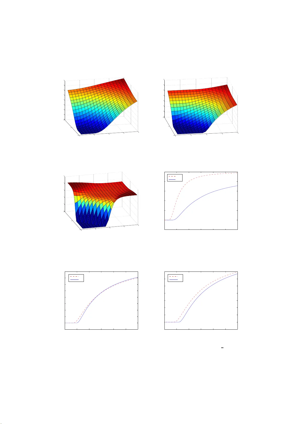
Optimal Uncertain t y Quan tificat ion H. Owhadi, T. J. Sulliv an, M. McKerns, M. Ortiz California Institute of T ec hnology o whadi@caltech.edu C. Sco vel Los Alamos National Lab orat ory jcs@lanl.gov Octob er 2 4, 2018 Abstract W e prop ose a rigorous framework for Uncertaint y Quantifi cation (UQ) in which the UQ ob jectives and the as sumptions/informatio n set are broug ht to the forefront. This framework, which we call O ptimal Unc ertainty Quantific ation (OUQ), is ba sed on the observ ation that, g iven a set of a s sumptions and info r mation ab out the problem, there exist optimal b ounds on uncerta in ties: these are o btained as v alues of well-defined optimization pro ble ms corr esp onding to extr e mizing proba bilities of failur e, or of dev ia tions, sub ject to the constraints imp o sed by the scenar io s compatible with the as s umptions and infor mation. In par ticular, this framework do es no t implicitly imp ose inappropriate assumptions, nor do es it r epudiate r elev ant information. Although OUQ optimization problems ar e extremely larg e, we show that un- der genera l conditions they have finite-dimensional reductions. As an application, we dev elo p Optimal Conc entr ation Ine qualities (OCI) of Ho effding and McDiarmid t y pe . Surprisingly , these results show that uncertainties in input parameters, which propaga te to output uncertainties in the classical sensitivity analysis para digm, may fail to do so if the transfer functions (or pr o bability distributions) are imp erfectly known. W e sho w ho w, for hier archical structures, this phenomeno n may lea d to the non-propag ation of uncertainties or information across scales. In addition, a general alg orithmic framework is dev elo ped for O UQ and is tested on the Caltech surroga te mo del for hypervelo city impact and on the seismic safety assessment of truss structures, suggesting the feasibility of the framework for im- po rtant complex systems. The introduction of this pap er pr ovides b oth an overview of the pap er and a self-contained mini-tutorial ab out basic c o ncepts and issues of UQ. 1 Con ten ts 1 In tro duction 4 1.1 The UQ p roblem . . . . . . . . . . . . . . . . . . . . . . . . . . . . . . . . 4 1.2 Motiv ating physica l example and outline of the pap er . . . . . . . . . . . 6 1.2.1 F orm ulation of the admissible set and redu ction theorems. . . . . . 8 1.2.2 Optimal concent ration inequalities. . . . . . . . . . . . . . . . . . . 10 1.2.3 Computational f ramew ork. . . . . . . . . . . . . . . . . . . . . . . 11 1.2.4 Outline of the pap er. . . . . . . . . . . . . . . . . . . . . . . . . . . 15 2 Optimal Uncertaint y Quantific ation 15 2.1 First description . . . . . . . . . . . . . . . . . . . . . . . . . . . . . . . . 16 2.2 The Optimal UQ lo op . . . . . . . . . . . . . . . . . . . . . . . . . . . . . 21 3 Generalizations and C omparisons 29 3.1 Prediction, extrap olation, v erifi cation and v alidatio n . . . . . . . . . . . . 29 3.2 Comparisons with other UQ metho d s . . . . . . . . . . . . . . . . . . . . . 30 3.3 OUQ with r andom sample d ata . . . . . . . . . . . . . . . . . . . . . . . . 33 4 Reduction of OUQ Optimization Problems 34 4.1 Reduction of O UQ . . . . . . . . . . . . . . . . . . . . . . . . . . . . . . . 35 4.2 Generalized momen ts of the resp ons e function . . . . . . . . . . . . . . . . 38 4.3 Application to McDiarmid’s inequalit y . . . . . . . . . . . . . . . . . . . . 40 5 Optimal Concentration Inequalitie s 43 5.1 Explicit solutions under the assu mptions of McDiarmid’s inequalit y . . . . 43 5.1.1 Explicit solutions in dimensions one and t wo . . . . . . . . . . . . 44 5.1.2 Explicit solution in d imension three . . . . . . . . . . . . . . . . . 44 5.1.3 Solution in dimension m . . . . . . . . . . . . . . . . . . . . . . . . 47 5.2 Explicit solutions under the assu mptions of Ho effding’s inequalit y . . . . . 48 6 Computational Implementation 49 6.1 Extreme p oints of reduced O UQ problems are attracto r s . . . . . . . . . . 49 6.2 Coagulation–F ragmen tation algorithm for OUQ . . . . . . . . . . . . . . . 49 6.3 The OUQ algorithm in the mystic framewo r k . . . . . . . . . . . . . . . . 53 7 Application to t he Seismic Safety Assessmen t of Structures 54 7.1 F ormulation in th e time domain . . . . . . . . . . . . . . . . . . . . . . . . 55 7.1.1 F ormulation of the p r oblem . . . . . . . . . . . . . . . . . . . . . . 55 7.1.2 F ormulation of the inf ormation set . . . . . . . . . . . . . . . . . . 56 7.1.3 The OUQ op timization p roblem . . . . . . . . . . . . . . . . . . . 58 7.1.4 Reduction of the optimization p roblem . . . . . . . . . . . . . . . . 58 7.1.5 Numerical r esults . . . . . . . . . . . . . . . . . . . . . . . . . . . . 58 7.2 OUQ and critical excitation. . . . . . . . . . . . . . . . . . . . . . . . . . . 62 7.3 Alternativ e form u lation in the frequency d omain . . . . . . . . . . . . . . 63 2 7.3.1 F ormulation of the inf ormation set . . . . . . . . . . . . . . . . . . 63 7.3.2 OUQ ob jectiv es . . . . . . . . . . . . . . . . . . . . . . . . . . . . . 64 7.3.3 Reduction of the optimization p roblem with Dirac masses . . . . . 65 7.3.4 Reduction of the optimization p roblem based on strong d ualit y . . 65 7.3.5 Numerical r esults . . . . . . . . . . . . . . . . . . . . . . . . . . . . 66 8 Application to T ransp ort in P orous Media 67 9 Conclusions 69 Ac kno w ledgemen ts 71 10 App endix: Proofs 71 10.1 Pro ofs for Section 4 . . . . . . . . . . . . . . . . . . . . . . . . . . . . . . 71 10.2 Pro ofs for Section 5 . . . . . . . . . . . . . . . . . . . . . . . . . . . . . . 75 References 83 3 1 In tro d uction 1.1 The UQ problem This pap er sets out a rigorous and unified framew ork for the statemen t and solution of uncertain ty quan tification (UQ) pr oblems cen tered on the n otion of a v ailable inf orm a- tion. In g eneral, UQ r efers to any attempt to quantita tivel y understand the relationships among uncertain parameters and processes in physical pr o cesses, or in m athematical and computational mo dels for them; suc h u nderstandin g may b e deterministic or probabilis- tic in nature. Ho wev er, to mak e the discuss ion sp ecific, we start the description of the prop osed framew ork as it applies to the certification pr oblem; S ection 3 giv es a b roader description of the pu rp ose, motiv ation and applications of UQ in the p rop osed framewo r k and a comparison with curr en t metho ds. By c ertific ation we mean the problem of sho w ing that, with probabilit y at least 1 − ǫ , the real-v alued resp ons e function G of a giv en physical system will not exceed a giv en safet y threshold a . That is, w e wish to sho w that P [ G ( X ) ≥ a ] ≤ ǫ. (1.1) In p r actice, the ev ent [ G ( X ) ≥ a ] ma y rep r esen t the crash of an aircraft, the failure of a w eap ons sys tem, or the av erage su rface temp erature on the Earth b eing to o high. The sym b ol P d enotes the pr obabilit y measure asso ciated with the randomness of (some of ) the inp ut v ariables X of G (commonly referred to as “aleat oric uncertain ty”) . Sp ecific examples of v alues of ǫ used in p ractice are: 10 − 9 in the a viation ind ustry (for the maxim um probabilit y of a catastrophic ev en t p er fligh t hour, see [ 83 , p .581] and [ 15 ]), 0 in the seismic design of nucle ar p ow er plants [ 28 , 23 ] and 0 . 05 for the collapse of s oil em bankm ents in surface mining [ 36 , p.358 ]. In structural engineering [ 31 ], the maxim u m p ermissib le probabilit y of failure (due to an y cause) is 10 − 4 K s n d /n r (this is an example of ǫ ) where n d is the design life (in y ears), n r is the n umber of people at risk in the eve nt of failure and K s is giv en b y the follo wing v alues (with 1 / y ear units): 0 . 005 for places of public safet y (including dams); 0 . 05 for d omestic, office or trade and indu stry structures; 0 . 5 for brid ges; and 5 for to wers, masts and offshore structures. In US en vironmental legislati on, the maximum acceptable increased lifetime c h ance of dev eloping cancer du e to lifetime exp osure to a su bstance is 10 − 6 [ 53 ] ([ 44 ] d ra ws atten tion to the fact that “there is n o sound scien tific, so cial , economic, or other basis for th e selection of the threshold 10 − 6 as a clean up goal for hazardous wa s te sites”). One of the m ost c h allenging asp ects of UQ lies in the fact that in practical appli- cations, the measure P and the resp onse function G are not kno wn a priori. This lac k of inform ation, commonly referred to as “epistemic uncertain ty”, can b e describ ed pre- cisely by introd ucing A , the set of all admissible sc enarios ( f , µ ) for the unkn o wn — or partially kno wn — realit y ( G, P ). More p recisely , in those applications, the a v ailable information d o es not determine ( G, P ) u ni q uely but ins tead determines a set A such th at an y ( f , µ ) ∈ A could a p riori b e ( G, P ). Hence, A is a (p ossib ly infinite-dimensional) s et of m easures and fu nctions defin ing explicitly information on and assumptions ab out G 4 Figure 1.1: Y ou ar e given one p ound of play-dough and a se esaw b alanc e d ar ound m . How much mass c an you put on right hand side of a while ke eping the se esaw b alanc e d ar ound m ? The solution of this optimization problem can b e ac hiev ed by placing an y mass on the right hand side of a , exactly at a (to place mass on [ a, 1] with minimum lev erage tow ards the righ t hand side of the seesaw) and an y m ass on the left hand side of a , exactly at 0 (for maximum leverag e to w ard s th e left hand side of the seesa w). and P . In practice, this set is ob tained from ph ysical la ws, exp erimen tal data and exp ert judgment. It then follo ws f rom ( G, P ) ∈ A that inf ( f ,µ ) ∈A µ [ f ( X ) ≥ a ] ≤ P [ G ( X ) ≥ a ] ≤ s up ( f ,µ ) ∈A µ [ f ( X ) ≥ a ] . (1.2) Moreo v er, it is element ary to observ e that • Th e quantit ies on the righ t-hand and left-hand of ( 1.2 ) are extreme v alues of optimization p roblems and element s of [0 , 1]. • Both the righ t-hand and left-hand in equalities are optimal in the sen s e that they are the sharp est b ou n ds for P [ G ( X ) ≥ a ] th at are consisten t with the information and assump tions A . More imp ortan tly , in Pr op osition 2.1 , w e s h o w th at these t wo inequalities p ro vide suffi- cien t information to pro d uce an optimal solution to the certification problem. Example 1.1. T o give a v ery simple example of the effect of inform ation and optimal b ound s o ver a class A , consider the certification p roblem ( 1.1 ) when Y := G ( X ) is a real-v alued r andom v ariable taking v alues in the interv al [0 , 1] and a ∈ (0 , 1); to further simplify the exp osition, w e consider only the upp er b oun d p roblem, sup press dep endence up on G and X and fo cus s olely on the question of w hic h pr obabilit y measures ν on R are admissible scenarios for the prob ab ility distribu tion of Y . So far, any p robabilit y measure on [0 , 1] is admissible: A = { ν | ν is a probabilit y measure on [0 , 1] } . and so the optimal up p er b ound in ( 1.2 ) is simply P [ Y ≥ a ] ≤ sup ν ∈A ν [ Y ≥ a ] = 1 . No w sup p ose that w e are giv en an additional p iece of in formation: th e exp ected v alue of Y equals m ∈ (0 , a ). These are, in fact , the assumptions corresp onding to an elemen tary 5 Mark o v in equalit y , and the corresp ondin g admissib le set is A Mrkv =  ν     ν is a probability measure on [0 , 1], E ν [ Y ] = m  . The least upp er b oun d on P [ Y ≥ a ] corresp onding to the admiss ible set A Mrkv is the solution of the infinite d imensional optimization problem sup ν ∈A Mrkv ν [ Y ≥ a ] (1.3) F ormulating ( 1.3 ) as a mec hanical optimization p roblem (see Figure 1.1 ), it is easy to observ e that the extremum of ( 1.3 ) ca n b e ac hieve d only considering the situation where ν is the weigh ted sum of mass a Dirac at 0 (with weig ht 1 − p ) and a mass of Dirac at a (with weigh t p ). It follo ws that ( 1.3 ) can b e reduced to the simp le (one-dimens ional) optimization p roblem: M aximize p subje ct to ap = m . It f ollo w s that Marko v’s in equ alit y is the optimal b oun d for the admissible set A Mrkv . P [ Y ≥ a ] ≤ sup ν ∈A Mrkv ν [ Y ≥ a ] = m a . (1.4) In some s ense, the OUQ framewo r k that w e p resen t in this pap er is the the extension of this pro cedu re to situ ations in whic h th e admissible class A is complicated enough that a closed-form inequ ality such as Mark o v’s inequalit y is u na v ailable, but optimal b ound s can nevertheless b e c ompute d using redu ction pr op erties analogous to the one illustrated in Figure 1.1 . 1.2 Motiv ating ph ysical example and outline of the pap er Section 2 gives a formal d escription of the Optimal Unc ertainty Quantific ation fr ame- w ork. In order to help intuitio n , we will illustrate and motiv ate our abstract defi nitions and results with a practical example: an analytical su rrogate mo d el for hyp erv elo city impact. The ph ysical system of in terest is one in whic h a 440C steel ball (4 40C is a stand ard, i.e. a grade of steel) of diameter D p = 1 . 778 mm impacts a 440C ste el plate of thic kness h (expressed in mm ) at sp eed v (e xp ressed in km · s − 1 ) at obliquity θ from the plate norm al. The physica l exp erimen ts are p erf ormed at the California Institute of T ec hnology SPHIR (Small Partic le Hyp erv elo cit y Impact Range) facilit y (see Figure 1.2 ). An analytical surrogate mo del w as devel op ed to appro ximate the p erforation area (in mm 2 ) caused b y this impact scenario. Th e surrogate resp onse fu nction is as f ollo ws: H ( h, θ , v ) = K  h D p  p (cos θ ) u  tanh  v v bl − 1  m + , (1.5) where the b al listic limit velo c ity (the sp eed b elo w wh ic h no p erforation area o ccurs) is giv en b y v bl := H 0  h (cos θ ) n  s . (1.6) 6 Figure 1.2: E xp erimenal set up. (a) Stainless steel spherical pr o jectile s and n ylon sab ots. (b) T arget plate held at the end of the gun b arrel (c) Perforatio n of the target plate (d ) General view of the Small Particle Hyp erv elo cit y Impact Range (SPHIR ) F acilit y at Caltec h (e) plate thic kn ess h , plate obliquit y θ and pro jectile vel o cit y v . The sev en quantit ies H 0 , s , n , K , p , u and m are fitting parameters that h a ve b een c hosen to minimize the least-squares error b etw een the surr ogate and a set of 56 exp erimental data p oin ts; they take the v alues H 0 = 0 . 5794 km · s − 1 , s = 1 . 4004 , n = 0 . 4482 , K = 10 . 3936 mm 2 , p = 0 . 4757 , u = 1 . 027 5 , m = 0 . 4682 . Hence, in this illustrativ e example, H ( h, θ , v ) will b e our resp onse function G ( X 1 , X 2 , X 3 ) and we will consider cases in which H is p erfectly and imp erfectly kno wn. In S ection 7 , we will apply the O UQ framework to the seismic safet y assessment of str uctures and consider a m ore complex example in v olving a large n u m b er of v ariables. 7 1.2.1 F orm ulation of the admissible set and reduction theorems. F or the example considered here, we will assume that the input p arameters h, θ and v are rand om v ariables, of unkn o wn pr obabilit y distribution P and of give n r ange ( h, θ , v ) ∈ X := X 1 × X 2 × X 3 , h ∈ X 1 := [1 . 5 24 , 2 . 667 ] mm = [60 , 105] mils , θ ∈ X 2 := [0 , π 6 ] , v ∈ X 3 := [2 . 1 , 2 . 8] km · s − 1 . (1.7) W e will m easur e lengths in b oth m m and mils (recall that 1 mm = 39 . 4 mils ). W e will adopt the “gunner ’s p ersp ectiv e” that failure consists of not p erforating the p late, and therefore seek to obtain an optimal b ound on th e pr obabilit y of n on- p erforation, i.e. P [ H ≤ 0], with p ossibly incomplete information on P and H . Assuming H to b e known, if the inf ormation on P is limited to the kno w ledge that v elo cit y , imp act obliquity and plate thic kn ess are indep end en t random v ariables a nd that the mean p erf oration area lies in a prescrib ed range [ m 1 , m 2 ] := [5 . 5 , 7 . 5] mm 2 , then th is information d escrib es the admissible set A H , wh ere A H :=    ( H , µ )       H give n by ( 1.5 ), µ = µ 1 ⊗ µ 2 ⊗ µ 3 , m 1 = 5 . 5 mm 2 ≤ E µ [ H ] ≤ m 2 = 7 . 5 mm 2    . (1.8) If the inform ation on H is limited to v alues of Osc i ( H ), the comp onen t-wise oscil- lations (defi n ed b elo w, it is a least upp er b ound on ho w a c hange in v ariable i affects the resp onse function), and if the inform ation on P is as ab o v e, then the corresp onding admissible s et is A McD , wh ic h corresp onds to the assumptions of McDiarmid’s inequalit y [ 57 ], and is defined by A McD :=    ( f , µ )       µ = µ 1 ⊗ µ 2 ⊗ µ 3 , m 1 = 5 . 5 mm 2 ≤ E µ [ f ] ≤ m 2 = 7 . 5 mm 2 , Osc i ( f ) ≤ Osc i ( H ) for i = 1 , 2 , 3    . (1.9) Definition 1.1. Let X := X 1 × · · · × X m and consider a fun ction f : X → R . F or i = 1 , . . . , m , we d efine the comp onent -w ise oscillations Osc i ( f ) := sup ( x 1 ,...,x m ) ∈X sup x ′ i ∈X i   f ( . . . , x i , . . . ) − f ( . . . , x ′ i , . . . )   . (1.10) Th us, Osc i ( f ) measur es the maximum oscillation of f in the i th factor. Remark 1.2. The explicit expression ( 1.5 ) of H and the ranges ( 1.7 ) allo w us to compute the comp onent-wise oscillati on s O sc i ( H ), w hic h are, resp ectiv ely , 8 . 86 m m 2 , 4 . 17 mm 2 and 7 . 20 mm 2 for thic kn ess, obliquity , and velocit y . 8 In general, for any admissible set A of fu nction/measure pairs for th e p erforation problem, we d efine U ( A ) := sup ( f ,µ ) ∈A µ [ f ( h, θ , v ) ≤ 0] . (1.11) In this notation, the optimal up p er b ounds on th e probabilit y of non-p erforation, giv en the inform ation con tained in A H and A McD , are U ( A H ) and U ( A McD ) resp ectiv ely . In A H the r esp onse fu nction is exactly kno wn w hereas in A McD it is imp erfectly kno wn (the information on the resp onse fu n ction is limited to its comp onent-wise oscil- lations Osc i ( H )). Both A H and A McD describ e epistemic un certain ties (sin ce in A H the probabilit y distrib utions of thic kness, obliqu ity , and v elocity are imp erfectly kno w n ). A McD is the set of resp ons e f unctions f and probabilit y measur es µ that could b e H and P giv en the information con tained in (i.e. the constrain ts imp osed b y) Osc i ( H ), the indep end ence of the input v ariables and the b oun ds m 1 and m 2 on the mean p erfora- tion area. U ( A McD ) q u an tifies the wo r st case scenario, i.e. the largest pr obabilit y of non-p erforation give n wh at H and P could b e. Reduction theorems. The optimization v ariables asso ciated w ith U ( A H ) are ten- sorizations of pr obabilit y measures on thic kness h , on obliquit y θ and velocit y v . Th is problem is not directly computational tractable since find ing the optim um app ears to re- quire a searc h o ver the spaces of probabilit y measures on the interv als [1 . 524 , 2 . 667] mm , [0 , π 6 ] and [2 . 1 , 2 . 8] km · s − 1 . Ho wev er, in S ection 4 (T h eorem 4.1 and Corollary 4.4 ) w e sho w that, since the constrain t m 1 ≤ E µ [ H ] ≤ m 2 is multi-l inear in µ 1 , µ 2 and µ 3 , th e optim um U ( A H ) can b e ac h iev ed by searc hing among those measures µ whose marginal distributions on eac h of th e three input p arameter ranges ha ve sup p ort on at most t wo p oints. That is, U ( A H ) = U ( A ∆ ) , (1.12) where the reduced feasible set A ∆ is give n by A ∆ :=        ( H , µ )         H giv en by ( 1.5 ), µ = µ 1 ⊗ µ 2 ⊗ µ 3 , µ i ∈ ∆ 1 ( X i ) for i = 1 , 2 , 3 , m 1 ≤ E µ [ H ] ≤ m 2        , (1.13) where ∆ 1 ( X i ) :=  αδ x 0 + (1 − α ) δ x 1   x j ∈ X i , f or j = 0 , 1 and α ∈ [0 , 1]  denotes the set of b inary con vex com binations of Dirac masses on X i . More generally , although the OUQ optimization p roblems ( 1.2 ) are extremely large, w e sh ow in Section 4 th at an im p ortan t sub class enjo ys significant and p r actical fin ite- dimensional reduction pr op erties. More pr ecisely , although th e op timization v ariables ( f , µ ) liv e in a pro d uct space of f unctions and probability m easures, for OUQ problems go v ern ed by linear inequalit y constrain ts on generalized momen ts, we demonstrate in Theorem 4.1 an d Corollary 4.4 that the searc h can b e reduced to one ov er probabilit y measures that are p ro du cts of finite con vex com b inations of Dirac m asses with explicit 9 upp er b ounds on th e num b er of Dirac masses. Moreo ver, all the results in this p ap er can b e extended to sets of extreme p oin ts (extremal measures) more general than Dirac masses, suc h as those describ ed by Dynkin [ 24 ]; we hav e phrased the results in terms of Dirac masses f or simplicit y . F u rthermore, when all constrain ts are generalized m omen ts of functions of f , the searc h o ver admissible f unctions reduces to a searc h o ve r functions on an m -fold pro du ct of finite d iscrete sp aces, and the searc h ov er m -fold pro d ucts of fi nite con vex com binations of Dirac masses reduce to the p ro ducts of pr obabilit y m easures on this m -fold pro duct of finite discrete spaces. This latter reduction, presente d in Theorem 4.7 , completely eliminates d ep endency on the coord inate p ositions of the Di rac masses. With th is result, the optimization v ariables of U ( A McD ) can b e redu ced to functions and p ro ducts of probabilit y measures on { 0 , 1 } 3 . 1.2.2 O ptimal concen tration inequalities. Concen tration-of-measure inequalities can b e used to obtain up p er b ound s on U ( A H ) and U ( A McD ); in that sense, th ey lead to sub-optimal metho ds. Indeed, according to McDiarmid’s inequalit y [ 57 , 58 ], for all fu nctions f of m indep enden t v ariables, one must ha ve µ  f ( X 1 , . . . , X m ) − E µ [ f ] ≥ a  ≤ exp  − 2 a 2 P m i =1 (Osc i ( f )) 2  . (1.14) Application of this inequalit y to ( 1.9 ) (using E µ [ f ] ≥ m 1 = 5 . 5 mm 2 ) yields the b ound U ( A McD ) ≤ exp − 2 m 2 1 P 3 i =1 Osc i ( H ) 2 ! = 66 . 4% . (1.15) Note th at U ( A McD ) := sup ( f ,µ ) ∈A McD µ [ f ≤ 0 ] is the least u pp er b ound on the p robabilit y of n on-p erforation P [ H = 0] giv en th e inform ation con tained in the admissible set ( 1.9 ). In Section 5 , the reduction tec h n iques of Section 4 are applied to obtain optimal McDiarmid and Ho effding inequalities, i.e. op timal concen tration-of-measure inequ ali- ties w ith the assum ptions of McDiarmid’s inequalit y [ 57 ] or Ho effding’s inequalit y [ 35 ]. In particular, Theorems 5.1 , 5.2 and 5.4 provide analytic solutions to the McDiarmid problem for dimen s ion m = 1 , 2 , 3, and Prop osition 5.7 p ro vides a recursive form u la for general m , thereby providing an optimal McDiarmid in equalit y in th ese cases. In Theorems 5.11 and 5.13 , w e giv e analytic solutions und er Hoeffd in g’s assump tions. A notew orthy result is that the optimal b ounds asso ciated with McDiarmid’s and Ho effd- ing’s assumptions are the same for m = 2 but ma y b e d istin ct for m = 3, and so, in some sen s e, inf ormation ab out linearit y or non-linearit y of the r esp onse function h as a differen t effect d ep endin g up on th e dimension m of the pr oblem. Non-propagation of uncertain ties. F or m = 2, defi n e A 2 to b e the space of all functions f and measure µ such that µ = µ 1 ⊗ µ 2 and Osc i ( f ) ≤ D i . The optimal 10 concen tration-of-measure inequ alit y with the assumptions of McDiarmid’s in equalit y , Theorem 5.2 , states that sup ( f ,µ ) ∈A 2 µ  f ( X 1 , X 2 ) − E µ [ f ] ≥ a  =            0 , if D 1 + D 2 ≥ a, ( D 1 + D 2 − a ) 2 4 D 1 D 2 , if | D 1 − D 2 | ≤ a ≤ D 1 + D 2 , 1 − a max( D 1 , D 2 ) , if 0 ≤ a ≤ | D 1 − D 2 | . (1.16) Observe that if D 2 + a ≤ D 1 , then the optimal b ound do es not d ep end on D 2 , and there- fore, an y d ecrease in D 2 do es not impr o ve th e inequalit y . These exp licit b ounds sh o w that, although un certain ties may pr opagate f or the true v alues of G and P (as exp ected from th e sensitivit y analysis paradigm), they ma y fail to do so when the information is incomplete on G and P and the ob jectiv e is the m aximum of µ [ f ≥ a ] compatible with th e giv en information. The non-pr opagation of input uncertaint ies is a non-trivial observ ation related to the fact that some of the constrain ts defining the range of th e input v ariables ma y n ot b e r ealized b y the worst-ca s e scenario (extrem um of the OUQ problem). W e ha ve further illustrated th is p oin t in Section 8 and sho wn that for sy s tems c haracterized by multi p le s cales or hierarc h ical structur es, information or uncertain ties ma y not pr opagate across scales. Note that the m = 2 case do es not apply to the SPHIR example (since ( 1.9 ) inv olv es thr ee v ariables, i.e. it requires m = 3). Application to the SPHIR facility admissible set ( 1.9 ) . F or m = 3, the “optimal McDiarmid inequalit y” of Theorem 5.4 and Remark 4.2 pr ovides the upp er b ound U ( A McD ) = 43 . 7% . (1.17) Remark 5.6 also sh ows that reducing the uncertain ty in obliquity (describ ed by the constrain t Osc i ( f ) ≤ Osc i ( H ) in ( 1.9 ) for i = obliquit y ) do es n ot affect the le ast u pp er b ound ( 1.17 ). Reca ll th at U ( A McD ) is the least upp er b ound on the probabilit y that the p erforation is zero giv en that the mean p erforation area is in b et we en 5 . 5 mm 2 and 7 . 5 mm 2 and the constrain ts imp osed b y the ind ep endence, ranges and comp onen t-wise oscillati ons asso ciated with the in put rand om v ariables. The difference b etw een ( 1.15 ) an d ( 1.17 ) lies in the fact that 66 . 4% is non-optimal whereas 43 . 7% is the le ast upp er b ound on the probability of non p erforation giv en the information con tained in A McD . 43 . 7% is a d irect f unction of the in formation conta in ed in A McD and Section 2 s ho ws ho w admissible sets with higher information con ten t lead to smaller lea st upp er b oun ds on the p robabilit y of non p erforation. Section 2 also s h o ws ho w such ad m issible sets can b e constructed, in th e OUQ framework, via the optimal selection of exp eriments. 1.2.3 C omputational framewo rk. With access to H , not just its comp onen t wise oscilla tions, ev en sharp er b ounds on the probabilit y of non-p erforation can b e calculated. Although we do not hav e an analytic al 11 (a) support points at iteration 0 (b) supp ort points at iteration 150 (c) su p p ort points at iteration 200 (d) support points at iteration 1000 Figure 1.3: F or # s upp( µ i ) ≤ 2 , i = 1 , 2 , 3, the maximizers of the OUQ pr oblem ( 1.12 ) asso ciated with the information set ( 1.8 ) collapse to t wo -p oin t (as opp osed to eigh t- p oint) supp ort. V elo city and obliquit y marginals eac h collapse to a single Dirac mass, while the plate thic kness marginal colla p ses to ha v e supp ort on the extremes of its range. Note the p erh aps su r prising r esult that the prob ab ility of non-p erf oration is maximized b y a distrib u tion supp orted on the minimal, n ot maximal, impact obliquit y . 12 Figure 1.4: Tim e ev olution of the genetic algorithm searc h for the OUQ pr oblem ( 1.12 ) asso ciated with the information set ( 1.8 ) (( 1.13 ) after redu ction) for #s u pp( µ i ) ≤ 2 for i = 1 , 2 , 3, as optimized by mystic . Thickness quic kly conv erges to the extremes of its range, w ith a weig ht of 0.621 at 60 mils and a weig ht of 0.379 at 105 mils . T h e degeneracy in obliqu it y at 0 causes th e fluctuations s een in the con vergence of obliqu it y w eight . Similarly , ve lo cit y con ve r ges to a single supp ort p oint at 2.289 km · s − 1 , the ballistic limit v elo cit y for thic kn ess 105 m ils and obliquit y 0 (see ( 1.6 )). (a) con vergence for thickness (b) con vergence for thic k ness weigh t (c) con vergence for obliquity (d) con vergence for obliquity weig ht (e) con vergence for velocit y (f ) con vergence fo r velocity weigh t 13 form u la f or U ( A H ), its calculation is made p ossible by the ident it y ( 1.12 ) derived fr om the reduction results of Section 4 . A numerica l optimization o v er th e finite-dimensional reduced feasible set A ∆ using a Differen tial Evo lution [ 72 ] optimization algorithm im- plemen ted in the mystic fr amework [ 60 ] (see Sub section 6.3 ) yields the follo wing optimal upp er b oun d on the p robabilit y of non-p erforation: P [ H = 0] ≤ U ( A H ) = U ( A ∆ ) n um = 37 . 9% . Observe that “ P [ H = 0] ≤ U ( A ) = U ( A ∆ )” is a theorem, whereas “ U ( A ∆ ) n um = 37 . 9%” is the outp u t of an algorithm (in this case, a genetic algorithm implemen ted in th e mystic fr amewo rk describ ed in Su b section 6.3 ). In p articular, its v alidit y is correlated with the efficiency of th e s p ecific algorithm. W e hav e introd uced th e sym b ol n um = to emphasize the distinction b etw een mathematical (in)equalities and n u merical outputs. Although we do not ha v e a theorem asso ciated with the co nv ergence of the numerical optimization algorithm, we ha ve a robust con trol ov er its efficiency b ecause it is applied to the fi nite dimensional problem U ( A ∆ ) instead of the infin ite optimization pr ob lem asso ciated with U ( A H ) (thanks to the r eduction theorems ob tained in Section 4 ). W e also observ e that the maximizer U ( A H ) can b e of significantly smaller dimension than that of th e elemen ts of U ( A ∆ ). In deed, for #sup p( µ i ) ≤ 2 , i = 1 , 2 , 3 (where #supp( µ i ) is the n u m b er of p oin ts form ing the su p p ort of µ i ), Figure 1.3 shows that n u merical sim u lations collapse to tw o-p oin t sup p ort: th e velocit y a nd obliquit y marginals eac h collapse to a single Dirac mass, and the plate th ic kness m arginal collapses to ha ve supp ort on the tw o extremes of its r ange. See Figure 1.4 for plots of the lo cations and w eight s of the Dirac masses form ing eac h marginal µ i as fu nctions of the num b er of iterations. Note that the lines for thickness and thickness weight are of the same color if they corr esp ond to the same sup p ort p oin t for the measure. In Section 6 we observ e that, ev en when a wider searc h is p erformed (i.e. o v er mea- sures with m ore than tw o-p oin t sup p ort p er marginal), th e calculated maximizers for these problems mainta in tw o-p oin t supp ort. This observ ation suggests that th e extreme p oints of the reduced O UQ problems are, in some sense, attractors and that adequate n u merical implemen tation of OUQ pr ob lems can d etect and use “hidden” redu ction prop erties ev en in the absence of theorems pro vin g them to b e tr u e. Based on these observ ations, we prop ose, in Section 6 , an OUQ optimization algorithm for arbitrary constrain ts based on a coagulation/fragmen tation of probabilit y distribu tions. The simula tions of Figures 1.3 and 1.4 sh o w that extremizers are singular and that their su pp ort p oin ts identify ke y pla yers, i.e. weak p oin ts of the system. In particular, for U ( A H ), the lo cation of the tw o-p oin t s upp ort extremizer sh o ws that reducing maximum obliquit y and the range of ve lo cit y will not decrease the optimal b ound on the pr ob ab ility of non p erforation, and suggests that reducing the uncertaint y in thic kn ess will decrease this b ound . In Section 2 , w e will show that the OUQ framewo rk allo ws the dev elopment of an OUQ loop that can b e used for exp er im ental design. In p articular, w e will sho w that th e problem of pred icting optimal b ounds on the results of exp eriments u nder th e assumption that the system is safe (or un safe) is w ell-p osed and b en efits from similar reduction prop erties as the certification pr oblem. Best exp eriments are then naturally 14 iden tified as those whose predicted ranges ha v e minimal o v erlap b et w een safe and unsafe systems. 1.2.4 O utline of the pap er. Section 2 formally describ es the Optimal U nc ertainty Qu antific ation framew ork and what it means to giv e optimal b ounds on the pr obabilit y of failure in ( 1.1 ) give n (lim- ited) information/assumptions ab out the system of in terest, and h ence how to rigorously certify or de-certify that system. Secti on 3 sho w s that many imp ortant UQ pr ob lems, suc h as pr ediction, v erification and v alidation, can b e formulate d as certification p rob- lems. S ection 3 also gives a comparison of OUQ with other widely used UQ metho ds. Section 4 s ho ws that although O UQ optimization pr oblems ( 1.2 ) are (a p riori) infi n ite- dimensional, they can (in general) b e redu ced to equiv alen t fi nite-dimensional p roblems in w hic h the optimization is ov er th e extremal scenarios of A and that the dimen sion of the redu ced problem is a fun ction of th e n u m b er of pr obabilistic inequ alities that describ e A . Ju st as a linear program finds its extreme v alue at the extremal p oin ts of a con ve x domain in R n , OUQ prob lems r educe to searc hes ov er fi nite-dimensional families of extremal scenarios. Section 5 app lies the resu lts of Section 4 to obtain optimal con- cen tration inequalities un der th e assumptions of McDiarmid’s inequalit y and Hoeffding’s inequalit y . Th ose in equalities show that, although uncertainti es ma y propagate for the true v alues of G and P , they might not w hen the information is incomplete on G and P . Section 6 discuss es the n umerical implementat ion of OUQ algorithms for the analytical surrogate mo del ( 1.5 ) for h yp erv elo cit y impact. Section 7 assesses the feasibilit y of the OUQ formalism by means of an application to the safety assessm en t of truss structur es sub jected to groun d motion excitation. This app lication con tains man y of the features that b oth m otiv ate and challenge UQ, includ ing imp erfect knowledge of random in puts of high dim en sionalit y , a time-dep enden t an d complex resp onse of the system, and the need to mak e high-consequence decisions p ertaining to the safet y of the system. S ection 8 applies th e OUQ fr amew ork and reduction th eorems of s ections 4 and 5 to d iv ergence form elliptic PDEs. A strikin g observ ation of Section 8 is that with incomplete informa- tion on the probabilit y distribu tion of the microstructur e, uncertain ties or information do not necessarily propagate across scales. Section 9 emp hasizes that the “UQ pr ob- lem”(as it is treated in common practice to da y) app ears to h a ve all the symptoms of an ill-p osed problem; and that, at the v er y least, it lac ks a coheren t general pr esen tation, m uch lik e the state of pr obabilit y theory b efore its rigorous formulat ion by Kolmogo r o v in the 1930s. It also stresses that OUQ is not the defi n itiv e answ er to th e UQ problem, but an op ening gam bit. Section 10 giv es the pro ofs of our main r esu lts. 2 Optimal Uncertain t y Quan tification In th is section, w e describ e more formally the Optimal Unc ertainty Q uantific ation f rame- w ork. In particular, w e describ e what it means to giv e optimal b oun ds on the pr obabilit y of failure in ( 1.1 ) giv en in f ormation/assumptions ab out the system of in terest, and h ence 15 ho w to rigorously certify or de-certify that s ystem. F or the sak e of clarit y , we will start the d escription of OUQ with deterministic information and assumptions (when A is a deterministic set of functions and probability measures). 2.1 First description In the OUQ paradigm, information and assumptions lie at the core of UQ: th e a v ailable information and assu m ptions describ e sets of admissible scenarios o ver which optimiza- tions w ill b e p erformed. As noted by Ho effdin g [ 34 ], assumptions ab out the s y s tem of in terest p la y a cen tral and s ensitiv e role in an y statistical d ecision problem, ev en though the assum p tions are often only appro xim ations of r ealit y . A simple example of an inform ation/assumptions set is giv en by constraining the mean and range of the resp onse fu n ction. F or example, let M ( X ) b e the set of probabilit y measures on the set X , and let A 1 b e the set of pairs of pr obabilit y measures µ ∈ M ( X ) and real- v alued measurable fun ctions f on X su c h that the mean v alue of f with r esp ect to µ is b and the diameter of the r ange of f is at most D ; A 1 :=        ( f , µ )         f : X → R , µ ∈ M ( X ) , E µ [ f ] = b, (sup f − inf f ) ≤ D        . (2.1) Let u s assum e that al l that w e kno w ab out the “realit y” ( G, P ) is that ( G, P ) ∈ A 1 . Then an y other pair ( f , µ ) ∈ A 1 constitutes an adm issible scenario r epresen ting a v alid p ossibilit y f or the “realit y” ( G, P ). If ask ed to b ound P [ G ( X ) ≥ a ], shou ld w e apply differen t metho ds and obtain d ifferen t b ounds on P [ G ( X ) ≥ a ]? Since s ome m etho ds will d istort this information s et and others are only u sing part of it, we instead view set A 1 as a feasible set f or an optimization problem. The general OUQ framework. In the general case, w e regard the r esp onse function G as an unknown measurable function, w ith some p ossibly kno wn charact er istics, from one measurable space X of inputs to a second measur able space Y of v alues. Th e inp ut v ariables are generated randomly according to an unknown random v ariable X with v alues in X according to a la w P ∈ M ( X ), also with some p ossib ly kno wn charac teristics. W e let a measurable sub set Y 0 ⊆ Y define the failur e r e gion ; in the example giv en ab o ve, Y = R and Y 0 = [ a, + ∞ ). When there is no danger of confusion, we shall simply write [ G fails] for the even t [ G ( X ) ∈ Y 0 ]. Let ǫ ∈ [0 , 1] d en ote the gr e atest ac c eptable pr ob ability of failur e . W e sa y that the system is safe if P [ G fails] ≤ ǫ and the s y s tem is unsafe if P [ G fails] > ǫ . By information , or a set of assumptions , w e mean a su bset A ⊆  ( f , µ )     f : X → Y is measurable, µ ∈ M ( X )  (2.2) 16 that con tains, at the least, ( G, P ). The set A enco des all the information th at w e h a ve ab out the r eal system ( G, P ), information that may come from kno wn p h ys ical la ws, past exp erimenta l d ata, and exp ert opinion. In the example A 1 ab o ve, the only information that we ha ve is that the mean r esp onse of the system is b and that th e diameter of its range is at most D ; any pair ( f , µ ) th at satisfies these tw o criteria is an admissible sc enario for the unkn o wn realit y ( G, P ). S ince some admissib le scenarios may b e s afe (i.e. h av e µ [ f fails ] ≤ ǫ ) whereas other admissible scenarios may b e uns afe (i.e. ha ve µ [ f fails] > ǫ ), w e decomp ose A in to the disjoin t union A = A safe ,ǫ ⊎ A unsafe ,ǫ , wh ere A safe ,ǫ := { ( f , µ ) ∈ A | µ [ f f ails] ≤ ǫ } , (2.3a) A unsafe ,ǫ := { ( f , µ ) ∈ A | µ [ f f ails] > ǫ } . (2.3b) No w observ e that, give n su c h an information/assumptions set A , there exist up- p er and low er b oun d s on P [ G ( X ) ≥ a ] corresp onding to the s cenarios compatible with assumptions, i.e. th e v alues L ( A ) and U ( A ) of the optimization problems: L ( A ) := inf ( f ,µ ) ∈A µ [ f fails] (2.4a) U ( A ) := sup ( f ,µ ) ∈A µ [ f fails] . (2.4b) Since L ( A ) and U ( A ) are well-defined in [0 , 1], and appr oximati on s are su fficien t for most p u rp oses a nd are n ecessary in general, the difference b et we en sup and max should not b e muc h of an issue. Of course, s ome of the work that follo ws is concerned with the attainmen t of maximizers, and wh ether those maximizers ha ve an y simp le structure that can b e exp loited for the sak e of computational efficiency , and this is the topic of Section 4 . F or the moment , h o we ver, sim p ly assume that L ( A ) and U ( A ) can in deed b e computed on demand. No w, sin ce ( G, P ) ∈ A , it follo ws that L ( A ) ≤ P [ G fails] ≤ U ( A ) . Moreo v er, the upp er b ound U ( A ) is optimal in the sense that µ [ f fails] ≤ U ( A ) for all ( f , µ ) ∈ A and, if U ′ < U ( A ), then there is an admissible scenario ( f , µ ) ∈ A suc h that U ′ < µ [ f fails] ≤ U ( A ) . That is, alt h ough P [ G fails] ma y b e m uch sm aller than U ( A ), there is a pair ( f , µ ) whic h satisfies the same assum ptions as ( G, P ) such th at µ [ f fails] is appro xim ately equal to U ( A ). S im ilar remarks apply f or the low er b ound L ( A ). Moreo v er, the v alues L ( A ) and U ( A ), defin ed in ( 2.4 ) can b e used to construct a solution to the certification problem. Let the certification pr oblem b e defined b y an error function that giv es an error w henev er 1) th e certification pro cess pro d u ces “safe” and there exists an admissible scenario that is u n safe, 2) the certification pro cess pro d uces 17 L ( A ) := inf ( f ,µ ) ∈A µ  f ( X ) ≥ a  U ( A ) := sup ( f ,µ ) ∈A µ  f ( X ) ≥ a  ≤ ǫ Cannot decide Insufficient Inform ation Certify Safe even in the W orst Case > ǫ De-certify Unsafe ev en in the Best Case Cannot decide Insufficient Inform ation T able 2.1: The OUQ certification pr o cess pr o vides a rigorous certification criterion whose outcomes are of three t yp es: “Certify”, “De-ce r tify” and “Cann ot decide”. “unsafe” and there exists an admissib le scenario th at is safe, or 3) the ce r tification pro cess pr o duces “cannot decide” and all admissib le scenarios are safe or all ad m issible p oints are unsafe; otherwise, the certification pro cess pro duces no error. The follo wing prop osition demonstrates that, except in the sp ecial case L ( A ) = ǫ , that th ese v alues determine an optimal solution to this certificatio n problem. Prop osition 2.1. If ( G, P ) ∈ A and • U ( A ) ≤ ǫ then P [ G fails ] ≤ ǫ . • ǫ < L ( A ) then P [ G fails ] > ǫ . • L ( A ) < ǫ < U ( A ) the ther e exists ( f 1 , µ 1 ) ∈ A and ( f 2 , µ 2 ) ∈ A such that µ 1 [ f 1 fails ] < ǫ < µ 2 [ f 2 fails ] . In other words, pr o vided th at the information set A is v alid (in the sens e that ( G, P ) ∈ A ) then if U ( A ) ≤ ǫ , then, the sys tem is pr o v ably safe; if ǫ < L ( A ), th en the system is pr o v ably u nsafe; and if L ( A ) < ǫ < U ( A ), then the s afet y of the system cannot b e decided due to lac k of information. The corresp ond ing certificatio n p ro cess and its optimalit y are represente d in T able 2.1 . Hence, s olving the optimization pr oblems ( 2.4 ) determines an optimal solution to the certification problem, un d er th e condition that L ( A ) 6 = ǫ . When L ( A ) = ǫ w e can still p ro duce an optimal solution if we obtain furth er information. That is, when L ( A ) = ǫ = U ( A ), then the optimal pr o cess pro d uces “safe”. On th e other hand, when L ( A ) = ǫ < U ( A ), the optimal solution d ep ends on whether or not there exists a minimizer ( f , µ ) ∈ A suc h that µ [ f fails] = L ( A ); if so, the optimal pro cess should declare “cannot d ecide”, otherwise, the optimal pro cess should d eclare “unsafe”. Observ e that, in T able 2.1 , w e h a v e classified L ( A ) = ǫ < U ( A ) as “cannot decide”. This “nearly optimal” solution app ears natur al and conserv ativ e without the kno wledge of the existence or non-existence of op timizers. Example 2.1. The b ounds L ( A ) and U ( A ) can b e computed exactly — an d are non- trivial — in the case of the simple example A 1 giv en in ( 2.1 ). Indeed, writing x + := max( x, 0), the optimal upp er b ound is given by U ( A 1 ) = p max :=  1 − ( a − b ) + D  + , (2.5) 18 where the maximum is ac hiev ed by taking the measur e of probabilit y of the r an d om v ariable f ( X ) to b e the w eigh ted sum of tw o w eight ed Dirac delta masses 1 p max δ a + (1 − p max ) δ a − D . This simple example demonstrates an extremely imp ortan t p oin t: ev en if the fu nction G is extremely exp ensiv e to ev aluate, certification can b e accomplished without recourse to the exp ensive ev aluations of G . F urth ermore, the simple structure of the maximizers motiv ates the reduction theorems later in S ection 4 . Example 2.2. As shown in Equ ation ( 1.14 ), concentrat ion-of-measure inequalities lead to sub-optimal metho ds in th e sense th at they can b e u sed to obtain u pp er b ound s on U ( A ) and lo we r b ounds on L ( A ). Observ e th at McDiarmid’s inequalit y ( 1.14 ) re- quired an information/assumptions set A McD where the space X is a pro duct space with X = ( X 1 , X 2 , . . . , X m ), the mean p erf ormance satisfies E [ G ( X )] ≤ b , the m inpu ts X 1 , . . . , X m are indep en d en t, and th e comp onent-wise oscillatio n s of G , (see ( 1.10 )) are b ound ed O sc i ( G ) ≤ D i . It follo ws fr om McDiarmid’s inequalit y ( 1.14 ) that, un der the assumptions A McD , U ( A McD ) ≤ exp  − 2 ( a − b ) 2 + P m i =1 D 2 i  . This example sho w s ho w existing tec hniqu es suc h as concentrati on-of-measure inequali- ties can b e incorporated in to OUQ. In Section 4 , w e will sh ow ho w to reduce U ( A McD ) to a finite dimens ional optimization problem. Based on th is reduction, in Section 5 , we pro- vide analytic solutions to the optimization problem U ( A McD ) for m = 1 , 2 , 3. In practice, the computation of the b oun ds D i require the resolution of an optimization problem, w e refer to [ 52 , 46 , 1 ] for practical metho ds. W e r efer to [ 52 , 46 , 1 , 78 ] for illustrations of UQ thr ough concent r ation of measure inequalities. In particular, sin ce Osc i ( G ) is a semi-norm, a (p ossibly n umerical) model can b e u sed to compute b ounds on comp onen t- wise oscil lations of G via th e triangular inequalit y Osc i ( G ) ≤ Osc i ( F ) + Osc i ( G − F ) (we refer to [ 52 , 46 , 1 ] for details, th e idea h ere is that an accurate mo del leads to a reduced n u m b er of exp eriments for the computation of Osc i ( G − F ), wh ile the computation of Osc i ( F ) do es not in volv e exp eriments). In the sequel w e will refer to D i,G := Os c i ( G ) (for i = 1 , . . . , m ) as the su b-diameters of G and to D G := v u u t m X i =1 D 2 i,G (2.6) as the diameter of G . Boun d s on Osc i ( G ) are useful b ecause th ey constitute a form of non-linear sensitivit y an alysis and, combined with ind ep enden ce constrain ts, they lead 1 δ z is the Dirac delta mass on z , i.e. the measure of probability on Borel subsets A ⊂ R such th at δ z ( A ) = 1 if z ∈ A and δ z ( A ) = 0 otherwise. The first Dirac delta m ass is lo cated at the minimum of the interv al [ a, ∞ ] (since w e are interested in maximizing the probabilit y of t he even t µ [ f ( X ) ≥ a ]). The second Dirac delta mass is lo cated at z = a − D b ecause we seek to maximize p max under the constraints p max a + (1 − p max ) z ≤ b and a − z ≤ D . 19 Admissible scenarios, A U ( A ) Metho d A McD : indep endence, oscillat ion and mean ≤ 66 . 4% McDiarmid’s inequalit y constrain ts as give n b y ( 1.9 ) = 43 . 7% T heorem 5.4 A H as giv en by ( 1.8 ) n um = 37 . 9% mystic , H kn o wn A H ∩  ( H , µ )     µ -median ve lo city = 2 . 45 k m · s − 1  n um = 30 . 0% mystic , H kn o wn A H ∩  ( H , µ )   µ -median obliquit y = π 12  n um = 36 . 5% mystic , H kn o wn A H ∩  ( H , µ )   obliquit y = π 6 µ -a.s.  n um = 28 . 0% mystic , H kn o wn T able 2.2: Summary of the u p p er b ound s on the pr obabilit y of non-p erforation for E x- ample ( 1.8 ) obtained b y v arious m etho ds and assumptions. Note that O UQ calculations using mystic (describ ed in Section 6 ) inv olv e ev aluations of the function H , whereas McDiarmid’s inequalit y and the optimal b ound giv en the assumptions of McDiarmid’s inequalit y use only the mean of H and its McDiarmid sub diameters, not H itself. Note also that the incorp oratio n of additional information/assumptions, e.g. on impact obliq- uit y , alw ays r educes the OUQ u pp er b oun d on th e probability of failure, since this cor- resp ond s to a restriction to a su bset of the original feasible set A H for the optimization problem. to the concen tration of measure phenomenon. Th e OUQ metho dology can also handle constrain ts of the t y p e k G − F k < C (whic h are n ot sufficien t to observ e tak e adv an tage of the concentrat ion of measure effect) and G ( x i ) = z i [ 90 ]. Example 2.3. F or th e set A H giv en in Equation ( 1.8 ), the inclusion of additional in- formation further reduces the upp er b ound U ( A H ). Indeed, the addition of assumptions lead to a smaller admissib le set A H 7→ A ′ ⊂ A H , therefore U decreases and L increases. F or example, if the median of the third input parameter (v elo cit y) is kno wn to lie at the midp oint of its range, and this information is used to provide an additional constraint, then the least upp er b ound on the pr obabilit y of non-p erforation d rops to 30 . 0%. See T able 2.2 for a summary of the b ounds p resen ted in the hyp erve lo city impact example in tro duced in S ubsection 1.2 , and for f urther examples of the effect of add itional infor- mation/constrain ts. T he b ounds giv en in T able 2.2 ha ve b een obtained b y us ing the reduction th eorems of Section 4 and the computational framew ork describ ed in Section 6 . Remark 2.2. The n u m b er of iterations and ev aluations of H asso ciated with T able 2.2 are: 600 iterations and 15300 H -ev aluations (second r o w), 822 iterations and 22700 H -ev aluations (third r o w), 515 iterations and 14550 H -ev aluations (fourth ro w ), 760 iterations and 18000 H -ev aluations (fifth r o w). Half of these n u m b ers of iterations are 20 usually suffi cien t to obtain the extrema w ith 4 digits of accuracy (for the third ro w, for instance, 365 iterations and 9350 H -ev aluations are sufficien t to obtain the fi rst 4 decimal p oints of the op timum). On the selectiv eness of the information set A . Ob serv e that, except for the b ound obtained from McDiarmid’s inequalit y , the b ounds obtained in T able 2.2 are the b est p ossible giv en the information con tained in A . If the unkn o wn d istribution P is completely sp ecified, sa y b y r estricting to the feasible set A unif for whic h th e only admissible measur e is the uniform probabilit y measur e on the cub e X (in whic h case the mean p erforation area is E [ H ] = 6 . 58 m m 2 ), then the probabilit y of non-p erforation is U ( A unif ) = L ( A unif ) n um = 3 . 8%. One ma y argue that there is a large gap b et w een the fifth (28%) row of T able 2.2 and 3 . 8% but observe th at 3 . 8% r elies on the exact kno wledge of G (called H h ere) and P wher eas 28% relies on the limited kn o wledge con tained in A H ∩  ( H , µ )   obliquit y = π 6 µ -a.s.  with resp ect to wh ic h 28% is optimal. In particular, the gap b et w een those t wo v alues is not caused by a lac k of tight n ess of the metho d, b ut by a lac k of selectiv eness of the inform ation con tained in A H ∩  ( H , µ )   obliquit y = π 6 µ -a.s.  . Th e (mis)use of the terms “tigh t” and “sharp” without reference to a v ailable inform ation (and in presence of asymmetric information) can b e the source of m u ch confu sion, something that we hop e is cleared up b y the pr esen t w ork. Giv en prior kn o wledge of G and P , it would b e an easy task to constru ct a set A P ,G con taining ( G, P ) suc h that U ( A P ,G ) ≈ 4% (if the p robabilit y of failure un der ( G, P ) is 3 . 8%), but d oing so w ou ld b e dela ying a h onest discussion on one of the issues at th e core of UQ: H ow to c onstruct A without prior know le dge of G and P ? In other w ords, ho w to impro ve the “selectiv eness” of A or ho w to d esign exp erimen ts leading to “narro w ” A s? W e will no w show ho w this question can b e addressed within th e OUQ fr amew ork. 2.2 The Optimal UQ lo op In the p r evious subsection w e d iscussed how the basic in equalit y L ( A ) ≤ P [ G ≥ a ] ≤ U ( A ) pro vid es rigorous optimal ce r tification crite r ia. The certification p ro cess sh ould n ot b e confused w ith its three p ossib le outcomes (see T able 2.1 ) whic h w e call “certify” (w e assert that the system is safe), “de-certify” (we assert that th e s y s tem is unsafe) and “cannot d ecide” (the s afety or un -safety of the system is und ecidable given the information/assumption s et A ). In deed, in the case L ( A ) ≤ ǫ < U ( A ) there exist admissible scenarios u nder wh ic h the system is s afe, and other admissible scenarios under whic h it is u nsafe. Consequent ly , it follo ws that w e can mak e no definite certification statemen t for ( G, P ) without in tro d ucing further information/assumptions. If n o fur ther information can b e obtained, we conclude that we “cannot decide” (this 21 Selection of New Exp erimen ts Exp erimental Data (Legacy / O n-Demand) Exp ert J udgemen t Ph ys ical La ws Assumptions / Ad missible Set, A Extreme Scale Optimizer: Calculate L ( A ) := inf { µ [ f f ails] | ( f , µ ) ∈ A } U ( A ) := sup { µ [ f f ails] | ( f , µ ) ∈ A} Certification Pro cess Sensitivit y / Robu s tness Analysis w.r .t. A De-Certify ( i.e. System is Unsafe) Cannot Decide Certify ( i.e. System is Safe) Figure 2.1: Optimal Un certain t y Q uan tification Lo op. state co uld also b e ca lled “do not decide”, b ecause w e could (arb itrarily) decide that the system is u nsafe du e to lac k of inform ation, for instance, but do n ot). Ho we ver, if sufficient resources exist to gather add itional in formation, then w e enter what ma y b e cal led the optima l unc ertainty quantific ation lo op , illustrated in Fi gure 2.1 . The admissible set A dr a ws on three principal sources of information: kno w n physic al la ws, exp ert opinion, and exp erimental data. Once th e set A has b een constructed, the calculation of the lo w er and up p er b ounds L ( A ) and U ( A ) are well- p osed optimiza- tion p roblems. If the results of these optimization p roblems lead to certification or de-certification, then we are d one; if n ot, then new exp eriments should b e designed and exp ert opinion sough t in order to v alidate or in v alidate the extremal sce n arios that cause the inequality L ( A ) ≤ ǫ < U ( A ) to h old. Th e addition of in f ormation means further constraints on the collection of 22 admissible scenarios; that is, the original adm issible set A is reduced to a s maller one A ′ ⊂ A , thereby p ro vidin g sharp er b ounds on th e probability of failure: L ( A ) ≤ L ( A ′ ) ≤ P [ G ( X ) ≥ a ] ≤ U ( A ′ ) ≤ U ( A ) . The s harp er b ound s ma y meet the “certify” or “decertify” criteria of T able 2.1 . If not, and there are still resources for gathering additional in formation, then the lo op should b e rep eated. This pro cess is the feedb ac k arr o w on the left-hand side of Figure 2.1 . The r igh t-hand side of Figure 2.1 constitutes another asp ect of the OUQ lo op. The b ound s L ( A ) and U ( A ) are only useful insofar as the assumptions A are accurate. It is p ossible that the s ou r ces of information that informed A m a y hav e b een in error: physic al la ws may ha ve b een extended outside their range of v alidit y (e.g. Newtonian physic s ma y h a v e b een app lied in the relativistic regime), there ma y hav e b een difficulties with the exp eriments or the results misin terp reted, or exp ert opinion ma y ha ve b een erroneous. Th erefore, a vital part of O UQ is to examine the sensitivit y and robustn ess of the b ounds L ( A ) and U ( A ) with resp ect to the assu mption s et A . If the b ounds L ( A ) and U ( A ) are found to dep end sensitiv ely on one particular assumption (sa y , the mean p erformance of one comp onent of the system), then it wo u ld b e advisable to exp end resources inv estigating th is assumption. The lo op illustrated in Figure 2.1 d iffers fr om the lo op u sed to solv e the numerical optimization prob lem as describ ed in Sub-section 6.3 and Remark 6.3 . Exp erimental design and selection of the most decisiv e exp erimen t. An im- p ortant asp ect of the OUQ lo op is the selection of new exp eriments. Supp ose that a n u m b er of p ossib le exp erimen ts E i are p rop osed, eac h of wh ic h will determine some func- tional Φ i ( G, P ) of G and P . F or example, Φ 1 ( G, P ) could b e E P [ G ], Φ 2 ( G, P ) could b e P [ X ∈ A ] for some sub set A ⊆ X of the inp ut parameter space, and so on. Su pp ose that there are insu fficien t exp erimen tal resources to run all of these prop osed exp eriments. Let us no w consider which exp eriment sh ould b e run for the certification problem. Recall that th e admissib le set A is partitioned into safe and unsafe sub sets as in ( 2.3 ). Defin e J safe ,ǫ (Φ i ) to b e the closed interv al s p anned by the p ossible v alues for the functional Φ i o v er the safe admissible scenarios (i.e. the closed con vex hull of the range of Φ i on A safe ,ǫ ): that is, let J safe ,ǫ (Φ i ) := " inf ( f ,µ ) ∈A safe ,ǫ Φ i ( f , µ ) , sup ( f ,µ ) ∈A safe , ǫ Φ i ( f , µ ) # (2.7a) J unsafe ,ǫ (Φ i ) := " inf ( f ,µ ) ∈A unsafe ,ǫ Φ i ( f , µ ) , sup ( f ,µ ) ∈A unsafe ,ǫ Φ i ( f , µ ) # . (2.7b) Note that, in general, these tw o interv als ma y b e disjoint or ma y h a ve non-empty inter- section; the size of their in tersection pro vides a m easure of u sefulness of the p rop osed exp eriment E i . Observe that if exp eriment E i w ere run , yielding the v alue Φ i ( G, P ), 23 then the follo wing conclusions could b e drawn: Φ i ( G, P ) ∈ J safe ,ǫ (Φ i ) ∩ J unsafe ,ǫ (Φ i ) = ⇒ no conclusion, Φ i ( G, P ) ∈ J safe ,ǫ (Φ i ) \ J unsafe ,ǫ (Φ i ) = ⇒ the system is safe, Φ i ( G, P ) ∈ J unsafe ,ǫ (Φ i ) \ J safe ,ǫ (Φ i ) = ⇒ the system is u nsafe, Φ i ( G, P ) / ∈ J safe ,ǫ (Φ i ) ∪ J unsafe ,ǫ (Φ i ) = ⇒ fault y assumptions, where the last assertion ( faulty assumptions ) means that ( G, P ) / ∈ A and follo ws from the fact that Φ i ( G, P ) / ∈ J safe ,ǫ (Φ i ) ∪ J unsafe ,ǫ (Φ i ) is a contradictio n . T he v alidit y of the first thr ee assertions is based on the su pp ositio n that ( G, P ) ∈ A . In this wa y , the computational optimization exercise of findin g J safe ,ǫ (Φ i ) and J unsafe ,ǫ (Φ i ) for eac h prop osed exp erimen t E i pro vid es an ob jectiv e assessment of whic h exp erimen ts are worth p erforming: those for whic h J safe ,ǫ (Φ i ) and J unsafe ,ǫ (Φ i ) are nearly disj oin t in terv als are w orth p erforming sin ce th ey are lik ely to yield conclusive results vis- ` a- vis (de-)certification and conv ersely , if the inte r v als J safe ,ǫ (Φ i ) and J unsafe ,ǫ (Φ i ) ha ve a large ov erlap, then exp erimen t E i is not wo r th p erforming since it is unlike ly to yield conclusiv e results. F urth ermore, the fourth p ossibility ab o ve shows h o w exp eriments can rigorously establish that one’s assumptions A are in corr ect. See Figure 2.2 for an illustration. Remark 2.3. F or the sak e of clarit y , we ha v e started this description by defi n ing ex- p eriments as functionals Φ i of P and G . In practice, some exp eriments ma y not b e functionals of P and G but of related ob jects. Consider, f or instance, the situation where ( X 1 , X 2 ) is a t wo- d imensional Gaussian v ector with zero m ean and cov ariance matrix C , P is the p r obabilit y d istribution of X 1 , the exp erimen t E 2 determines the v ariance of X 2 and the information set A is C ∈ B , where B is a su b set of symmetric p ositiv e defi nite 2 × 2 matrices. The outcome of the exp erimen t E 2 is not a function of the pr obabilit y distribution P ; ho wev er, the knowledge of P r estricts the range of p ossi- ble outcomes of E 2 . Hence, for some exp erimen ts E i , the knowledge of ( G, P ) do es not determine the outcome of the exp er im ent, but only the set of p ossible outcomes. F or those exp eriments, the description giv en ab o v e can b e generalized to situations wh ere Φ i is a multivalue d f u nctional of ( G, P ) determining the set of p ossible outcomes of the exp eriment E i . This p icture can b e generalized fur ther b y introdu cing measurement noise, in whic h case ( G, P ) ma y not d etermin e a d eterministic set of p ossible outcomes, but instead a measure of probabilit y on a set of p ossible outcomes. Example 2.4 (Compu tational solution of the exp erimen tal s election problem) . W e will no w consider again the admissible set A H as give n by ( 1.8 ). The follo wing example sho ws that the n otion of “b est” exp eriment dep ends on the admiss ib le safet y th reshold ǫ for P [ G ≥ a ]. Sup p ose that an exp eriment E is p rop osed that will determine the p roba- bilit y mass of the u pp er half of the v elocity range, [2 . 45 , 2 . 8] km · s − 1 ; the corresp ondin g functional Φ of study is Φ( µ ) := µ [ v ≥ 2 . 45 km · s − 1 ] , and th e p rop osed exp erimen t E will determine Φ( P ) (appro x im ate determinations includ- ing measurement and sampling err ors can also b e handled, bu t the exact determination 24 R J unsafe ,ǫ (Φ 1 ) J safe ,ǫ (Φ 1 ) R J unsafe ,ǫ (Φ 2 ) J safe ,ǫ (Φ 2 ) R J unsafe ,ǫ (Φ 3 ) J safe ,ǫ (Φ 3 ) R J unsafe ,ǫ (Φ 4 ) J safe ,ǫ (Φ 4 ) Figure 2.2: A sc hematic r ep resen tation of the in terv als J unsafe ,ǫ (Φ i ) (in red) and J safe ,ǫ (Φ i ) (in blue) as defined by ( 2.7 ) for four fu nctionals Φ i that migh t b e the sub ject of an exp erimen t. Φ 1 is a go o d candidate for exp eriment effort, since the int er v als do not o v er lap and hence exp erimen tal d etermination of Φ 1 ( G, P ) w ill certify or de-certify the system; Φ 4 is not w orth in vestig ating, since it cannot distinguish safe scenarios fr om unsafe ones; Φ 2 and Φ 3 are inte rmediate cases, and Φ 2 is a b etter p rosp ect than Φ 3 . is done here f or simplicit y). Th e corresp onding int erv als J safe ,ǫ (Φ) and J unsafe ,ǫ (Φ) as defined by ( 2.7 ) and ( 2.3 ) are rep orted in T able 2.3 f or v arious acceptable probabilities of failure ǫ . Note that, for larger v alues of ǫ , E is a “b etter” exp eriment in the sense that it can d istinguish safe scenarios from unsafe on es (see also Figure 2.2 ); for smaller v alues of ǫ , E is a p oor exp eriment. In an y case, since the in tersection J safe ,ǫ (Φ) ∩ J unsafe ,ǫ (Φ) is not emp t y , E is not an ideal exp eriment. It is imp ortan t to note that the optimization calculations necessary to compu te the in terv als J safe ,ǫ (Φ) and J unsafe ,ǫ (Φ) are simplified b y the application of Theorem 4.1 : in this case, the ob jectiv e f unction of µ is µ [ v ≥ 2 . 45] ins tead of µ [ H = 0], but the constrain ts are once again linear inequalities on generalize d moments of the optimization v ariable µ . On t he n umber of total ev aluat ions on H . Rec all that, for simplicit y , w e ha ve assumed the resp onse function G to b e known and giv en by H . A large num b er of ev aluations of H has b een u sed in T able 2.3 to ensur e con verge n ce tow ards th e global optim um. It is imp ortan t to observ e th at those ev aluations of H are not (actual, costly) exp eriments but (c heap) numerical ev aluations of equation ( 1.5 ). More precisely , the 25 J safe ,ǫ (Φ) J unsafe ,ǫ (Φ) inf sup inf sup ǫ = 0 . 100 0 . 000 1 . 000 0 . 000 0 . 900 iterations until numerica l conv ergence 40 40 40 30 0 total ev aluations of H 1 , 000 1 , 000 1 , 000 8 , 000 ǫ = 0 . 200 0 . 000 1 . 000 0 . 000 0 . 800 iterations until numerica l conv ergence 40 40 40 40 0 total ev aluations of H 1 , 000 1 , 000 1 , 000 12 , 000 ǫ = 0 . 300 0 . 000 1 . 000 0 . 000 0 . 599 iterations until numerica l conv ergence 40 40 40 1000 total ev aluations of H 1 , 000 1 , 000 1 , 000 33 , 000 T able 2.3: The resu lts of the calculation of the inte rv als J safe ,ǫ (Φ) and J unsafe ,ǫ (Φ) for the functional Φ( µ ) := µ [ v ≥ 2 . 45 km · s − 1 ]. Note that, as the acceptable probabilit y of system failure, ǫ , increases, the tw o in terv als o ve r lap less, so exp erimen tal determination of Φ( P ) w ould b e more likel y to yield a decisive conserv ativ e certificati on of th e system as safe or uns afe; the computational cost of th is in creased d ecisive n ess is a greater n u mb er of function ev aluations in the optimization calculat ions. All computational cost figur es are appr o ximate. metho d for selecting n ew b est exp eriments do es not require new exp erimen ts; i.e., it relies entirely on the information set A (which contai ns the inform ation gathered fr om previous exp erimen ts). Hence th ose ev aluations sh ould not b e viewe d as “information gained from Mon te Carlo samp les” but as “pur e CPU pro cessing time”. In situations where the n u merical ev aluation of H is exp ensiv e, one can in tro duce its cost in the optimization lo op. An inv estigatio n of the b est algorithm to p erform the numerical optimization with the least n umber of function ev aluations is a worth while sub ject b ut is b eyo n d th e scop e of the present p ap er. Observe also that the metho d prop osed in Section 2 do es not rely on the exact kn o wledge of the resp on s e fu nction G . Mo re precisely , in situations w here the resp onse f unction is unknown, the selection of next b est exp erimen ts is still en tirely computational, and based up on previous d ata/information ga thered on G enforced as constrain ts in a numerical optimizatio n algorithm. More pr ecisely , in those situations, th e optimization algorithm ma y r equire the n u merical ev aluation of a large n u m b er of admissib le f unctions f (compatible w ith the prior information a v ailable on G ) but it do es n ot require any new ev aluation of G . In situations where H is (n umerically) exp ensive to ev aluate, one would ha ve to include the cost of these ev aluations in the optimization lo op and us e fast algorithms exploiting the m ulti-linear structures asso ciated with the computatio n of safe and u n safe in terv als. Here w e h a ve used a genetic algorithm b eca use its r obustness. This algorithm t ypically con verges at 10% of the total num b er of ev aluations of H give n in the last row 26 Figure 2.3: A schemati c represen tation o f the size of the predictio n in terv als sup outcomes c  U ( A E , c ) − L ( A E , c )  in the worst case with resp ect to outcome c . E 4 is the most p r edictiv e exp eriment. of T able 2.3 but we ha ve increased the n umber of it erations tenf old to guaran tee a r obust result. The inv estigatio n of efficien t optimization algorithms exp loiting the m u lti-linear structures of OUQ op timization problems is of great interest and b ey ond the immediate scop e of this pap er. Selection of the most predictive exp erimen t. Th e compu tation of safe a nd unsafe in terv als describ ed in the previous paragraph allo ws of the selection of the most selectiv e exp eriment. If our ob jectiv e is to ha ve an “accurate” prediction of P [ G ( X ) ≥ a ], in the sense that U ( A ) − L ( A ) is small, then one can pro ceed as foll o ws. Let A E , c denote those scenarios in A that are compatible w ith obtaining outcome c from exp er im ent E . An exp eriment E ∗ that is most pred ictiv e, ev en in the wo r st case, is defined by a minmax criterion: w e seek (see Figure 2.3 ) E ∗ ∈ arg min experiments E  sup outcomes c  U ( A E , c ) − L ( A E , c )   (2.8) The idea is that, although w e can not predict the precise outcome c of an exp erimen t E , w e can compute a wo rst-case scenario w ith resp ect to c , and obtain an optimal b ound for the minimum decrease in our prediction in terv al for P [ G ( X ) ≥ a ] based on the (yet unknown) information gained from exp eriment E . Again, th e th eorems giv en in this pap er can b e app lied to reduce th is kind of prob lem. Findin g E ∗ is a bigger pr oblem than jus t calculating L ( A ) and U ( A ), bu t the pr esumption is that computer time is c heap er than exp erimen tal effort. Planning of campaigns of exp eriments. The idea of exp erimen tal selection can b e extended to plan seve r al exp eriments in adv ance, i.e. to p lan campaigns of exp eri- men ts. This asp ect can b e u sed to assess the safet y or the design of complex systems in a minimal num b er of exp erimen ts (and also to predict b ounds on the total num b er of required exp eriments). Just as a go o d chess pla y er thinks sev eral mo ves ahead, our framew ork allo ws for the design of increasingly soph isticated an d optimal sequences of exp eriments that can b e p erformed to measure key system v ariables. The implemen- tation of this s trategy corresp onds to a min max game “pla yed against the Un iv erse” 27 (a) Pla ying Chess against the universe (b) Let’s play Clue, Round 1 (c) Let’s play Clue, Round 2 (d) Let’s play Clue, Round 3 Figure 2.4: Subfigur e (a) : Pla ying C hess Against the Univ erse. W e c h o ose w hic h ex- p eriment E to p erform and the universe selects the outcome c . Our ob jectiv e is to minimize U ( A ) − L ( A ) . In the fir s t roun d our p ossib le mov es corresp ond to a c h oice b et ween exp erimen ts E 1 , E 2 , E 3 and E 4 . W e p erform exp eriment E 4 , th e outcome c of that exp eriment (selected b y the Unive r se) transforms the admiss ib le in to A E 4 ,c . In the second round, our p ossible mo ves corresp ond to a c h oice b et ween exp eriments F 1 , F 2 and F 3 . As in the game of Chess, sev eral mov es can b e p lann ed in adv ance by solving min max optimizatio n p r oblems, and the exp onenti al in crease of the num b er branches of the game tree can b e k ep t under con trol b y exploring only a su bset of (b est) mo ves. Subfi gures (b) , (c) and (d) : Let’s pla y Clu e. 28 (Subfigur e 2.4(a) ). The well -kn o wn games of Clue/Cluedo and Tw ent y Qu estions are b etter analogies than c h ess for this kind of inform ation game. In that sense, the plan- ning of campaigns of exp erimen ts is an in finite-dimensional C lu e, p la y ed on sp aces of admissible scenarios, against our lac k of p erf ect inform ation ab out realit y , and m ade tractable b y the reduction theorems. This aspect calls for more inv estigation since it has the p oten tial to provide a new approac h to the curren t scien tific in vestig ation paradigm, whic h is b ased on intuitio n , exp ert j udgment , and guessing. Example 2.5 (Let’s pla y Clue.) . In Su bfigures 2.4(b) , 2.4(c) and 2.4(d) we consider again the admissible set A H as giv en by ( 1.8 ) and select three most predictiv e exp eri- men ts, sequenti ally , choosing the second one after ha vin g observ ed the outcome of the first on e. The list of p ossible exp eriments corresp ond s to measuring the mean or v ari- ance of thickness h , obliquity θ or velocit y v . S ubfigur es 2.4(b) , 2.4(c) and 2.4(d) sho w U ( A H,E ,c ) for eac h of these exp er im ents as a function of the re-normalized outcome v alue c . Since, in this example, we alw a ys ha ve L ( A H,E ,c ) = 0, U ( A H,E ,c ) corresp onds to the size of th e prediction in terv al for the probabilit y of non-p erforation give n the in- formation that the outcome of exp erimen t E is c . Giv en the r esults sho w n in S ubfigur e 2.4(b) we select to measure the v ariance of thic kn ess as our first b est exp erimen t. Note that this selection do es n ot require the kn o wledge of what the exp eriment wil l yield but only the kn owledge of what th e exp erimen t c an yield: w e id entify as the optimal next exp eriment the one that is most inform ativ e in th e minimax sense, i.e. of all its p ossible outcomes (this do es not require the kno wledge of what the exp eriment will yield), its least inf ormativ e outcome is more inf ormativ e than th e least informativ e outcome of an y other candidate exp erimen t. Although not necessary , this selecti on can, p ossibly , b e guided b y a mo del of realit y (i.e. in this case a mo del for the p robabilit y distribu tions of h, θ , v ). Use d in this manner , an accurate mo d el will redu ce the n u m b er of exp eri- men ts requir ed f or certification and an inaccurate m o del will lead to a relativ ely greater n u m b er of exp eriments (bu t not to err on eous b ound s). Subfigur e 2.4(c) is b ased on the information con tained in A H and b ound s on the v ariance of thic kness (obtained f r om the first exp erimen t). Our selectio n as second exp eriment is to m easur e the mean of thic kness (leading to Sub figure 2.4(d) ). 3 Generalizations and Comparisons 3.1 Prediction, extr ap olation, ve rification and v alidation In the p revious section, the OUQ f r amew ork was describ ed as it applies to th e the certification p roblem ( 1.1 ). W e will no w sh o w that man y imp ortant UQ problems, suc h as prediction, v erification and v alidatio n , can b e form ulated as certification pr oblems. Th is is similar to th e p oin t of view of [ 5 ], in which formulatio n s of man y p r oblem ob jectiv es in reliabilit y are sho wn to b e r ep resen table in a u nified framework. A prediction problem can b e form u lated as, giv en ǫ and (p ossibly incomplete) information on P and G , findin g a smallest b − a suc h that P [ a ≤ G ( X ) ≤ b ] ≥ 1 − ǫ, (3.1) 29 whic h , giv en the admissib le set A , is equiv alen t to solving inf  b − a     inf ( f ,µ ) ∈A µ [ a ≤ f ( X ) ≤ b ] ≥ 1 − ǫ  . (3.2) Observe that [ a, b ] can b e interpreted as an optimal in terv al of confidence for G ( X ) (although b − a is minimal, [ a, b ] ma y not b e u n ique), in particular, with p robabilit y at least 1 − ǫ , G ( X ) ∈ [ a, b ]. In man y applications the regime where exp erimen tal d ata can b e tak en is differen t than the deplo ym en t regime w here pr ed iction or certification is sough t, and this is com- monly referred to as the extrapolat ion problem . F or example, in materials mo deling, exp erimenta l tests are p erformed on materials, and the mo d el run for comparison , bu t the d esir e is that these results tell us something where exp erimen tal tests are imp ossible, or extremely exp ensive to obtain. In most applications, the r esp onse function G may b e appr o ximated via a (p ossibly n u merical) mod el F . Information on the relation b et w een the mo del F and the resp onse function G that it is d esigned to r epresen t (i.e. information on ( x, F ( x ) , G ( x ))) can b e used to restrict (constrain) th e set A of admissible scenarios ( G, P ). Th is information ma y tak e the form of a b oun d on s ome d istance b et w een F and G or a b ound on some complex fu nctional of F and G [ 52 , 78 ]. Ob s erv e th at, in th e con text of the certification problem ( 1.1 ), th e v alue of the mo del can b e m easured by changes induced on the optimal b ounds L ( A ) and U ( A ). The problem of quantifying the relation (p ossibly the distance) b etw een F and G is commonly referred to as the v alidation problem . In some situations F ma y b e a numerical mo d el in vol vin g millions of lines of co de and (p ossibly) space-time discretization. The quantificat ion of the uncertaint y asso ciated with th e p ossible presence of b ugs and d iscretizatio n approximat ions is commonly referred to as the v erification problem . Both, the v alidation and the verificatio n p r oblem, can b e addressed in the OUQ fr amew ork by in tro d ucing inf ormation sets describing r elations b et ween G , F and the co de. 3.2 Comparisons w it h other UQ metho ds W e w ill no w compare OUQ with other widely used UQ m etho ds and consider the certi- fication problem ( 1.1 ) to b e sp ecific. • Assu me th at n indep enden t samples Y 1 , . . . , Y n of th e random v ariable G ( X ) are a v ailable (i.e. n indep enden t observ ations of the random v ariable G ( X ), all dis- tributed according to the measure of p robabilit y P ). If 1 [ Y i ≥ a ] denotes the random v ariable equal to one if Y i ≥ a and equal to zero otherwise, then p n := P n i =1 1 [ Y i ≥ a ] n (3.3) is an un b iased estimator of P [ G ( X ) ≥ a ]. F u r thermore, as a resu lt of Ho effding’s concen tration inequ alit y [ 33 ], the probability that p n deviates from P [ G ( X ) ≥ n ] 30 (its mean) by at least ǫ/ 2 is b oun ded from ab o ve by exp( − n 2 ǫ 2 ). It follo ws th at if the n u m b er of samples n is large en ou gh (of th e order of 1 ǫ 2 log 1 ǫ ), then the certifica tion of ( 1.1 ) can b e obtained through a Mon te Carlo estimate (u s ing p n ). As this example shows, Mon te Carlo strategies [ 50 ] are sim p le to implemen t and d o not necessitate prior information on the resp onse function G and the measure P (ot her than th e i.i.d. s amples). Ho wev er, they require a large n u m b er of (indep enden t) samples of G ( X ) which is a sev ere limitation for the certification of rare ev ents (the ǫ = 10 − 9 of the a viation indu stry w ould [ 83 , 15 ] necessitate O (10 18 ) samples). Additional inf orm ation on G an d P can, in principle, b e in cluded (in a limited fashion) in Mon te Carlo strategie s via imp ortance and we ighted samp ling [ 50 ] to reduce th e n u m b er of required samples. • Th e num b er of required samples can also b e redu ced to 1 ǫ (ln 1 ǫ ) d using Quasi- Mon te Carlo Metho ds . W e refer in p articular to the Koksma–Hla wk a inequalit y [ 64 ], to [ 82 ] for multiple in tegration based on lattice ru les and to [ 81 ] for a recent review. W e observ e that these metho ds r equire some regularit y (differentia bilit y) condition on the resp onse function G and the p ossibility of sampling G at pr e- determined p oints X . F u r thermore, the n u m b er of requ ir ed samples blows-up at an exp onen tial rate with the dimension d of the inpu t v ector X . • If G is r egular enough and can b e s amp led at at pre-determined p oin ts, and if X has a known distrib ution, then sto c hastic expansion metho ds [ 30 , 29 , 101 , 4 , 26 , 19 ] can r educe the n umb er of r equ ired samples even fur ther (dep end ing on the regu- larit y of G ) provided that the d imension of X is not to o h igh [ 94 , 14 ]. Ho wev er, in most applications, only in complete inf orm ation on P and G is a v ailable and the num b er of a v ailable samples on G is sm all or zero. X ma y b e of high d imen- sion, and ma y include uncon trollable v ariables and unkn o wn unkn owns (unknown input parameters of the resp onse fu nction G ). G may not b e th e solution of a PDE and ma y inv olv e inte r actions b etw een singular and complex pro cesses such as (for instance) dislo cation, fragmen tation, phase tr an s itions, physical p h enomena in unteste d regimes, and even human decisions. W e observe that in man y app li- cations of Sto chastic Exp ansion metho ds G and P are assumed to b e p erfectly kno wn and UQ redu ces to computing the pu sh forward of the measure P via the resp onse (transfer) fun ction I ≥ a ◦ G (to a measure on t wo p oin ts, in those situations L ( A ) = P [ G ≥ a ] = U ( A )). • Th e inv estigatio n of v ariations of the resp onse function G under v ariations of the input parameters X i , commonly referr ed to as sensitivit y analysis [ 75 , 76 ], allo ws for the identificati on of critical input parameters. Although helpful in estimating the r ob u stness of conclusions made b ased on sp ecific assump tions on input pa- rameters, sensitivit y analysis, in its most general form, has not b een targeted at obtaining rigorous upp er b ound s on pr obabilities of f ailur es asso ciated with cer- tification problems ( 1.1 ). Ho w ever, single parameter oscillati on s of the fu nction G (as defined by ( 1.10 )) can b e seen as a form of non-linear sen s itivit y analysis leading to b ounds on P [ G ≥ a ] via McDiarmid’s concent ration inequalit y [ 57 , 58 ]. 31 These b ounds can b e made sh arp b y partitioning the input parameter sp ace along maxim um oscil lation directions an d co m p uting sub-diameters on sub-domains [ 91 ]. • If A is expr essed probabilistically through a prior (an a priori measure of p robabil- it y) on the set p ossible s cenarios ( f , µ ) then Ba y esian inference [ 48 , 7 ] could in principle b e used to estimate P [ G ≥ a ] using the p osterior measure of probabilit y on ( f , µ ). This com bination b et w een OUQ and Ba ye sian metho d s av oids the ne- cessit y to solv e the p ossib ly large optimization problems ( 2.4 ) and it also greatly simplifies the incorp oration of sampled data thanks to the Ba y es r ule. Ho we ver, often times, priors are not a v ailable or their c hoice in vo lv es some degree of arbi- trariness that is incompatible with the certification of rare eve nts. Pr iors may b ecome asymptotically ir relev ant (in the limit of large data sets) but, for small ǫ , the n u m b er of required samples can b e of the same order as the num b er r equired b y Mon te-Carlo metho ds [ 79 ]. When unknown parameters are estimated u sing p riors and sampled data, it is im- p ortant to obs er ve that th e conv ergence of the Ba y esian metho d ma y fail if the underlying probability mec hanism allo ws an in finite num b er of p ossible outcomes (e.g., estimation of an unknown p robabilit y on N , the set of all natur al num b ers) [ 17 ]. I n fact, in these in finite-dimensional situations, this lac k of conv ergence (com- monly referr ed to as inconsistency) is th e rule rather than the exception [ 18 ]. As emphasized in [ 17 ], as mor e data c omes i n, some Bayesian statisticians wil l b e c ome mor e and mor e c onvinc e d of the wr ong answer . W e also obs er ve that, for complex systems, the compu tation of p osterior p robabil- ities h as b een m ade p ossible th anks to adv ances in computer science. W e refer to [ 89 ] for a (recen t) general (Gaussian) framew ork for Ba yesia n in verse pr ob lems and [ 6 ] for a rigorous UQ framew ork based on prob ab ility logic with Ba ye s ian up dating. Just as Ba y esian metho ds would hav e b een considered computationally infeasible 50 years ago b ut are now common practice, OUQ metho d s are now b ecoming fea- sible and will only increase in feasibilit y w ith th e passage of time and adv ances in computing. • Th e com bin ation of structur al optimization (in v arious fields of en gineering) to pro du ce an optimal design given th e (deterministic) worst-c ase scenario has b een referred to as Optimization and An t i-Optimization [ 27 ] (we also refer to crit- ical excitation in seismic engineering [ 21 ]). The main difference b etw een OUQ and An ti-optimization lies in the f act that the f orm er is based on an optimization o v er (admissible) functions and measures ( f , µ ), w hile the latter only in vol v es an optimization ov er f . Because of its robustness, many engineers ha ve adopted the (deterministic) w orst-case scenario approac h to UQ (w e refer to c hapter 10 of [ 27 ]) when a high reliabilit y is requir ed . It is n oted in [ 27 ] that the reason why pr ob- abilistic metho ds do not find appr e ciation among the or eticians and pr actitioners alike lies in th e fact that “probabilistic reliabilit y s tudies inv olv e assu mptions on the pr obabilit y densities, wh ose knowle d ge r egarding relev an t inp ut quan tities is cen tral”. It is also observed that strong assump tions on P ma y lead to GIGO 32 (“garbage in –garbage out”) situations for small certification thresholds ǫ when re- liabilit y estimates and probabilities of failure are v er y s ensitiv e to small deviations in pr obabilit y densities. On the other hand, UQ metho d s based on determin istic w orst-case scenarios are often times “to o p essimistic to b e p ractical” [ 21 , 27 ]. W e suggest that by allo wing for v ery w eak assumptions on probability measures, OUQ metho ds can lead to b ound s on p robabilities of failure that are b oth r eliable and practical. Indeed, when applied to complex sys tems in volving a large num b er of v ariables, d etermin istic worst-ca se metho d s do not tak e int o account the impr ob a- bility that these (p ossibly in dep end en t or wea kly correlated) v ariables conspire to pro du ce a failure eve n t. The certification pr oblem ( 1.1 ) exhibits one of th e main difficulties that face UQ practitioners: man y theoretica l m etho ds are a v ailable, b u t they r equ ire assum ptions or conditions that, often times, are not satisfied by the app lication. More p recisely , the c haracteristic elemen ts distinguish ing these different metho ds are the assumptions up on whic h they are based, and some m etho ds w ill b e more efficien t than others dep ending on the v alidit y of those assumptions. UQ app lications are also c h aracterized b y a set of assumptions/information on the resp onse fun ction G and measure P , whic h v aries from application to application. Hence, on the one h and, w e hav e a list of theoretica l metho d s that are applicable or efficien t und er v ery sp ecific assumptions; on the other hand, most applications are c haracterized by an in formation set or assump tions that, in general, do not matc h those r equired b y these theoretical metho ds. It is hence natural to pur s ue the dev elopment of a rigorous framework that d o es n ot add inappropr iate assum p tions or discard inf ormation. W e also observ e that the effectiv eness of d ifferen t UQ metho d s cann ot b e compared without reference to the a v ailable information (some methods will b e m ore effici ent than others d ep endin g on those assum ptions). F or the hyp erve lo city impact example of Sub- section 1.2 , none of the metho d s menti on ed ab o v e can b e used without adding (arb itrary) assumptions on probabilit y d ensities or discardin g information on th e mean v alue or in- dep end ence of th e input parameters. W e also observe that it is by placing inform ation at the cen ter of UQ that the p r op osed OUQ framework allo ws f or the iden tification of b est exp erimen ts. Without fo cus on the a v ailable information, UQ metho d s are faced with the risk of propagating inapp ropriate assumptions and pro ducing a soph isticated answ er to the wrong question. T h ese distortions o f th e inform ation set ma y b e of limite d impact on certificati on of common ev en ts but they are also of critical imp ortance for the certification of rare ev ents. 3.3 OUQ with random sample data F or the sak e of clarit y , w e hav e started the description of OUQ with d eterministic infor- mation and assumptions (i.e. when A is a deterministic set of f unctions and probabilit y measures). I n m an y app licatio ns, ho wev er, some of the information arriv es in the form of random samples. The addition of s u c h samp le d ata to the a v aila ble in formation and assump tions leads to n on-trivial theoretical questions that are of practical imp or- 33 tance b eyond their fundamenta l connections with inf ormation theory and n onparametric statistics. In particular, while the notion of an optimal b oun d ( 2.4 ) is tran s paren t and unam biguous, th e notion of an optimal b ound on P [ G ( X ) ≥ a ] in presence of sample data is not immediately ob vious and should b e treate d with care. This is a v ery delicate topic, a fu ll treatmen t of whic h w e shall d efer to a fu ture wo r k. 4 Reduction of OUQ Optimization Problems In general, the lo wer and up p er v alues L ( A ) := inf ( f ,µ ) ∈A µ [ f ( X ) ≥ a ] U ( A ) := sup ( f ,µ ) ∈A µ [ f ( X ) ≥ a ] are eac h d efined b y a non-conv ex and infinite-dimensional optimization problem, th e so- lution of whic h p oses signifi can t computational challenge s . Th ese optimization problems can b e considered to b e a generaliza tion of Chebyshev inequalities. The h istory of the classical inequalities can b e found in [ 42 ], and some generalizat ions in [ 13 ] an d [ 9 8 ]; in the latter w ork s , the conn ection b etw een Chebyshev inequalities and optimization theory is dev elop ed b ased on the work of Mulholland and Rogers [ 62 ], Godwin [ 32 ], Isii [ 37 , 38 , 39 ], Olkin and Pratt [ 65 ], Marshall an d Olkin [ 54 ], and the classical Mark ov–Krein T h eorem [ 42 , p ages 82 & 157], among others. The Chebyshev-t yp e inequalities d efined by L ( A ) and U ( A ) are a further generalization to ind ep endence assum ptions, more general do- mains, more general s ystems of momen ts, and the inclusion of classes of functions, in addition to the prob ab ility measures, in th e optimization p roblem. Moreo v er, although our goal is the computation of th ese v alues, and not an analytic expression for them, the study of pr obabilit y inequalities should b e useful in the reduction and ap p ro ximation of these v alues. Without pro viding a su rve y of th is large b o dy of wo r k, w e menti on the field of ma jorizatio n, as d iscussed in Marshall and Olkin [ 55 ], th e inequalities of And erson [ 3 ], Ho effd ing [ 33 ], Jo e [ 40 ], Bentkus et al. [ 11 ], Ben tkus [ 9 , 10 ], Pin elis [ 69 , 70 ], and Bouc heron, Lugosi and Massart [ 16 ]. Moreo v er, the solution of the r esulting noncon v ex optimization problems sh ould b enefit fr om d ualit y theories for nonconv ex optimization problems su c h as Ro c k afella r [ 74 ] and the d ev elopment of con ve x en velopes f or them, as can b e foun d, for example, in Rikun [ 73 ] and Sherali [ 80 ]. Finally , since P ard alos and V av asis [ 67 ] show th at quadratic programming with one negativ e eigen v alue is NP-hard, w e exp ect th at some OUQ p r oblems ma y b e d ifficult to solv e. Let us n o w retur n to the earlier simple example of an admissible set A 1 in ( 2.1 ): the (non-unique) extremizers of the OUQ problem w ith the admissible set A 1 all hav e the prop erty that the sup p ort of the pu sh-forward measur e f ∗ µ on R con tains at most tw o p oints, i.e. f ∗ µ is a con ve x com bination of at most tw o Dirac delta measures (we recall that #sup p( f ∗ µ ) is the n u m b er of p oints form in g the supp ort of f ∗ µ ): sup ( f ,µ ) ∈A 1 µ [ f ( X ) ≥ a ] = sup ( f ,µ ) ∈A 1 #supp( f ∗ µ ) ≤ 2 µ [ f ( X ) ≥ a ] . 34 The optimization problem on the left-hand s ide is an infinite-dimensional one, w hereas the optimization problem on the right -hand side is amenab le to fin ite-dimensional parametriza- tion for eac h f . F urthermore, for eac h f , only the t wo v alues of f at the s upp ort p oint s of the t wo Dirac measures are relev an t to the p roblem. The aim of th is section is to sho w that a large class of O UQ problems — those go verned b y ind ep endence and linear inequalit y constrain ts on the momen ts, — are amenable to a similar finite-dimensional reduction, and that a priori up p er b ound s can b e giv en on the n um b er of Dirac delta masses that the reduction requ ires. T o b egin with, we first show that an imp ortan t class of optimizatio n p roblems o v er the space of m -fold pro duct measures can b e reduced to optimizatio n ov er pro du cts of finite conv ex co mbinations o f Dirac masses ( m is the n umber of random inpu t v ariables). Consequent ly , we then sh o w in Corollary 4.4 that O UQ optimization pr oblems where the admissible set is d efined as a subset of function-measure pairs ( f , µ ) that satisfy gen- eralized m omen t constraints G f ( µ ) ≤ 0 can also b e reduced from the space of m easures to the p ro ducts of finite con vex combinatio n s of Dirac masses. Theorem 4.7 shows that, when all the constrain ts are generalized momen ts of functions of f , the searc h space G of fun ctions can b e further reduced to a searc h o ver fun ctions on an m -fold pro du ct of finite discrete spaces, and the search o ve r m -fold p ro ducts of fi nite con vex combinatio n s of Dirac masses can b e reduced to a searc h o ve r th e pro ducts of probabilit y measur es on this m -fold pro du ct of fi nite discrete spaces. T his latter reduction completely eliminates dep end ency on th e coord inate p ositions in X . Th eorem 4.7 is then used in Prop ositio n 4.8 to obtain an optimal McDiarmid inequalit y thr ou gh the f orm u lation of an appro- priate OUQ optimization pr oblem follo wed by the ab o ve-men tioned redu ctions to an optimization problem on th e pro du ct of f unctions on { 0 , 1 } m with the m -fold p ro ducts of measures on { 0 , 1 } m . This pr ob lem is then further red uced, by Theorem 4.9 , to an optimization pr oblem on the pr o duct of the space of s ubsets (p ow er set) of { 0 , 1 } m with the pro du ct measures on { 0 , 1 } m . Finally , we obtai n analytic solutions to th is last p rob- lem for m = 1 , 2 , 3, thereby obtaining an optimal McDiarmid inequalit y in these cases. W e also obtain an asymptotic form u la for general m . Moreo ver, the solution for m = 2 indicates important information regarding the diameter p arameters D 1 and D 2 (w e refer to Example 2.2 ). F or examp le, if D 2 is su fficien tly smaller than D 1 , then the optimal b ound only dep ends on D 1 and therefore, any decrease in D 2 do es not improv e the inequalit y . See S ubsection 10.1 for the pr o ofs of the r esu lts in this section. 4.1 Reduction of OUQ F or a top ological space X , let F X (or simply F ) denote the space of real-v alued (Borel) measurable functions on X , and let M ( X ) denote the set of Borel probabilit y measures on X . Denote the pro cess of integ r ation w ith resp ect to a measure µ by E µ , and let ∆ k ( X ) :=    k X j =0 α j δ x j       x j ∈ X , α j ≥ 0 for j = 0 , . . . , k and k X j =0 α j = 1    35 denote the set of ( k + 1)-fold conv ex com binations of Dirac masses. When X = Q m i =1 X i is a pr o duct of top ological spaces, an d w e sp eak of measurable fu n ctions on the pro du ct X , we mean m easur able with resp ect to the p ro du ct σ -algebra and not the Borel σ - algebra of th e p ro duct. F or more discussion of th is d elicate topic, see e.g. [ 41 ]. Th e linear equalit y and inequality constraints on our optimization pr oblems w ill b e enco ded in the follo wing measurable fun ctions: g ′ j : X → R for j = 1 , . . . , n ′ , and, for eac h i = 1 , . . . , m , g i j : X i → R for j = 1 , . . . , n i . Let M G ⊆ M m ( X ) denote the set of pro du cts of Borel measures for whic h these all these functions are integrable with finite integrals. W e use th e compact notation G ( µ ) ≤ 0 to indicate that µ ∈ M G and that E µ [ g ′ j ] ≤ 0 , for all j = 1 , . . . , n ′ , E µ [ g i j ] ≤ 0 , j = 1 , . . . , n i , f or all i = 1 , . . . , m . Moreo v er, let r : X → R b e inte grable for all µ ∈ M G (p ossibly with v alues + ∞ or −∞ ). F or an y set M ⊆ M G , let U ( M ) := sup µ ∈M E µ [ r ] , with the con ve ntion that the su premum of the empt y s et is −∞ . F or a m easur able f u nction f , the m ap µ 7→ E µ [ f ] ma y not b e d efi ned, since f may not b e absolutely integ r able with r esp ect to µ . If it is defined, th en it is con tinuous in the strong top ology on measures; ho wev er, th is top ology is to o str on g to pro vid e any compactness. Moreo ve r, although [ 2 , Theorem 14.5] s h o ws that if f is a b ounded upp er semi-con tin u ous f unction on a m etric sp ace, then integrat ion is up p er semi-con tinous in the weak- ∗ top ology , we consider the case in whic h X m a y not b e m etric or compact, and the functions f m a y b e unb ounded and lac k con tinuit y prop erties. The follo w ing results hea vily use results of Winkler [ 10 0 ] — wh ic h follo w from an extension of Cho quet Theory (see e.g. [ 68 ]) by von W eizs¨ ac k er and Winkler [ 99 , Corollary 3] to sets of prob- abilit y measures with generalized momen t constraints — and a result of Kendall [ 45 ] c haracterizing cones, whic h are latt ice cones in their o wn ord er. These results generaliz e a result of Karr [ 43 ] that r equires X to b e compact, the constrain t fu nctions b e b ounded and con tin u ous, and the constr aints to b e equ alities. Th e results th at follo w are r emark- able in that th ey mak e extremely wea k assump tions on X and n o assumptions on the functions f . Recall that a S uslin space is the cont inuous image of a Polish space. Theorem 4.1. L et X = Q m i =1 X i b e a pr o duct of Suslin sp ac es and let M m ( X ) := m O i =1 M ( X i ) 36 denote the set of pr o ducts of Bor el pr ob ability me asur e s on the sp ac es X i . As ab ove, c onsider the gene r alize d moment functions G and the c orr e sp onding finite moment set M G . Supp ose that r : X → R is inte gr able for al l µ ∈ M G (p ossibly with values + ∞ or −∞ ). Define the r e duc e d admissible set M ∆ := ( µ ∈ m O i =1 ∆ n i + n ′ ( X i )      G ( µ ) ≤ 0 ) . Then, it holds that U ( M G ) = U ( M ∆ ) . Theorem 4.1 sa ys that, on a pro duct X of v ery general spaces X i , optimization prob- lems constrained by n ′ linear momen t constrain ts on X and n i linear momen t co n strain ts on eac h factor s p ace X i ac hiev e their optima among those pro du ct measures whose i th marginal has su pp ort on at m ost n ′ + n i + 1 p oints of X i . Remark 4.2. Using [ 99 , Corollary 3], th is theorem and its consequences b elo w easily generalize f rom th e situation where E µ [ g k ] ≤ 0 f or eac h k to th at in which E µ [ g k ] ∈ I k for eac h k , w here k in dexes th e constraint fun ctions, and where eac h I k is a closed int er v al. Consequent ly , such pairs of linear constraints introdu ce a requiremen t for only on e Dirac mass, not the tw o masses that one might exp ect. Moreo ve r, observ e that the condition that the fu nction r is in tegrable (p ossib ly w ith v alues + ∞ or −∞ ) for all µ ∈ M G is satisfied if r is non-negativ e. In particular, th is holds when r is an indicator function of a set, w hic h is our main application in this p ap er. Remark 4.3. Theorem 4.1 and its consequents b elo w can b e expressed more generally in terms of extreme p oints of sets of measur es, w hereas in the ab o v e case, the extreme p oints are the Dirac m asses. T o that end, Dynkin [ 24 ] describ es more general sets of measures and their extreme p oints, wh ic h can b e usefu l in applications. In p articular, one could consider 1. sets of measur es that are in v arian t un der a trans formation (the extreme p oin ts are the ergo dic measures); 2. symm etric measures on an infin ite p r o duct space (the extreme p oin ts are the simple pro du ct measures); 3. the set of stationary distrib u tions for a giv en Mark ov transition f u nction; 4. the set of all Mark o v pro cesses with a giv en transition function. W e n o w apply Theorem 4.1 to obtain the same typ e of redu ction for an admissible set A ⊆ F × M m ( X ) consisting of pairs of functions and pr o duct measures — this is the case for th e OUQ optimization problems L ( A ) and U ( A ). Let G ⊆ F den ote a sub set of real-v alued measurable fu nctions on X and consider an admissible set A ⊆ G × M m ( X ) defined in the follo wing w a y . F or eac h f ∈ G , let G ( f , · ) denote a f amily of constrain ts as in Theorem 4.1 and Remark 4.2 . F or eac h f ∈ G , let M G f ⊆ M m ( X ) denote those p ro duct probabilit y measures µ suc h that th e moments G ( f , µ ) are w ell-defined . 37 Moreo v er, f or eac h f ∈ G , let r f : X → R b e in tegrable for all µ ∈ M G f (p ossibly with v alues + ∞ or − ∞ ). Define th e admissible s et A := { ( f , µ ) ∈ G × M m ( X ) | G ( f , µ ) ≤ 0 } (4.1) and defin e the OUQ optimization problem to b e U ( A ) := sup ( f ,µ ) ∈A E µ [ r f ] . (4.2) Corollary 4.4. Consider the OU Q optimization pr oblem ( 4.2 ) and define the r e duc e d admissible set A ∆ ⊆ A by A ∆ := ( ( f , µ ) ∈ G × m O i =1 ∆ n i + n ′ ( X i )      G ( f , µ ) ≤ 0 ) . ( 4.3) Then, it holds that U ( A ) = U ( A ∆ ) . Remark 4.5. Corollary 4.4 is easily generalized to the case w h ere for eac h f ∈ G , i , and fixed µ j , j 6 = i , G ( f , µ 1 , .., µ i , .., µ m ) has affin e dimension at most m i as µ i v aries. In this case A ∆ := ( ( f , µ ) ∈ G × m O i =1 ∆ m i ( X i )      G ( f , µ ) ≤ 0 ) . Remark 4.6. Linear moment constraints on the factor spaces X i allo w to consider information sets w ith indep enden t random v ariables X 1 , . . . , X m and w eak constrain ts on th e pr obabilit y measure of the v ariables X i . An example of suc h an admissible set is the one asso ciated with Bernstein inequ alities [ 12 ], in which a p riori b ound s are giv en on the v ariances of the v ariables X i . 4.2 Generalized momen ts of the r esp onse function W e n o w consider the case where the function r f := r ◦ f is defined through comp osition with a measurable fu nction r , and all n constraints are determined by comp ositio ns g ′ j := g j ◦ f , with j = 1 , . . . , n , of the function f . Hence, the symbol G ( f , µ ) will mean that all fun ctions g j ◦ f are µ integ r able and will represent the v alues E µ [ g j ◦ f ] for j = 1 , . . . , n . T hat is, we hav e th e admissible s et A := { ( f , µ ) ∈ G × M m ( X ) | G ( f , µ ) ≤ 0 } (4.4) and the optimization pr oblem U ( A ) := sup ( f ,µ ) ∈A E µ [ r ◦ f ] (4.5) as in ( 4.2 ). Ho we ver, in this case, the fact that the criterion function r ◦ f and the constrain t functions g j ◦ f are comp ositions of the function f p ermits a finite-dimensional 38 reduction of the s pace of fun ctions G to a space of f unctions on { 0 , . . . , n } m and a reduction of the space of m -fold pro d ucts of fin ite conv ex com bin ations of Dirac masses to the space of pro d uct measures on { 0 , . . . , n } m . This reduction completely eliminates dep end ency on the co ordin ate p ositions in X . F ormulating this result p r ecisely will require s ome additional n otation. By the W ell- Ordering T heorem, there exists a w ell-ordering of eac h X i . Supp ose that a total ordering of th e elements of the sp aces X i for i = 1 , . . . , m is sp ecified. Let N := { 0 , . . . , n } and D := { 0 , . . . , n } m = N m . Every element µ ∈ N m i =1 ∆ n ( X i ) is a pro du ct µ = N m i =1 µ i where eac h factor µ i is a conv ex sum of n + 1 Dirac m asses indexed according to the ordering; that is, µ i = n X k =0 α i k δ x k i for some α i 1 , . . . , α i n ≥ 0 with unit sum and some x 1 i , . . . , x n i ∈ X i suc h th at, with resp ect to the giv en ordering of X i , x 1 i ≤ x 2 i ≤ · · · ≤ x n i . Let F D denote the real linear space of real functions on D = { 0 , . . . , n } m and consider the mapp ing F : F × m O i =1 ∆ n ( X i ) → F D defined by ( F ( f , µ )) ( i 1 , i 2 , . . . , i m ) = f ( x i 1 1 , x i 2 2 , . . . , x i m m ) , i k ∈ N , k = 1 , . . . , m . F represent s the v alues of the fun ction f at the Dirac masses in µ , bu t d o es not carry information regardin g th e p ositions of the Dirac masses or th eir w eigh ts. Theorem 4.7. Consider the admissible set A and optimization pr oblem U ( A ) define d in ( 4.4 ) and ( 4.5 ) wher e r ◦ f is inte gr able (p ossibly with values + ∞ or −∞ ) for al l pr o duct me asur es. F or a subset G D ⊆ F D , define the admissible set A D = { ( h, α ) ∈ G D × M m ( D ) | E α [ g i ◦ h ] ≤ 0 for al l j = 1 , . . . , n } (4.6) and the optimization pr oblem U ( A D ) := sup ( h,α ) ∈A D E α [ r ◦ h ] . If F G × m O i =1 ∆ n ( X i ) ! = G D , then it holds that U ( A ) = U ( A D ) . When the constrain t set also in cludes fun ctions wh ich are not comp ositions with f , then T h eorem 4.7 do es not apply . Although it do es app ear that results sim ilar to Theorem 4.7 can b e obtained, we leav e that as a topic for fu ture wo r k. 39 4.3 Application t o McDiarmid’s inequalit y Theorem 4.7 can b e app lied to the situation of McDiarmid’s inequalit y in order to ob tain an optimal solution for th at problem. Let D i ≥ 0 for i = 1 , . . . , m and defi n e G := { f ∈ F | Osc i ( f ) ≤ D i for eac h i = 1 , . . . , m } , (4.7) where Osc i ( f ) := sup ( x 1 ,...,x m ) ∈X sup x ′ i ∈X i   f ( . . . , x i , . . . ) − f ( . . . , x ′ i , . . . )   . W e hav e a pro duct probability measur e P on X and a m easurable fun ction H : X → R suc h that H ∈ G . Su pp ose that we ha ve an up p er b oun d P [ H − E P [ H ] ≥ a ] ≤ H ( a, G ) for all H ∈ G . (4.8) It follo ws that if H ∈ G an d E P [ H ] ≤ 0, th en P [ H ≥ a ] ≤ P [ H − E P [ H ] ≥ a ] ≤ H ( a, G ) for all H ∈ G with E P [ H ] ≤ 0 . On the other hand, sup p ose that P [ H ≥ a ] ≤ H ′ ( a, G ) for all H ∈ G with E P [ H ] ≤ 0 . (4.9) It follo ws that P [ H ≥ a ] ≤ H ′ ( a, G ) for all H ∈ G with E P [ H ] = 0 . Since the constraints G and th e even t H − E P [ H ] ≥ a are in v arian t under scalar translation H 7→ H + c it follo ws that P [ H − E P [ H ] ≥ a ] ≤ H ′ ( a, G ) for all H ∈ G . That is, th e inequalities ( 4.8 ) and ( 4.9 ) are equ iv alen t. McDiarmid’s inequalit y [ 57 , 58 ] provides the b ound H ( a, G ) := exp ( − 2 a 2 D 2 ) for ( 4.8 ) and its equiv alen t ( 4.9 ), w ith D 2 := m X i =1 D 2 i . (4.10) Define the adm issible set corresp ondin g to the assump tions of McDiarmid’s in equalit y: A McD = { ( f , µ ) ∈ G × M m ( X ) | E µ [ f ] ≤ 0 } , (4.11) and defin e the optimization p roblem U ( A McD ) := s u p ( f ,µ ) ∈A McD µ [ f ≥ a ] . (4.12) 40 Since ( H , P ) ∈ A McD and McDiarmid’s inequalit y µ [ f ≥ a ] ≤ exp( − 2 a 2 D 2 ) is s atisfied for all ( f , µ ) ∈ A McD , it follo ws that P [ H ≥ a ] ≤ U ( A McD ) ≤ exp  − 2 a 2 D 2  . Moreo v er, th e inequalit y on the left is optimal in the sen s e th at, for every ε > 0, there exists a McDiarmid-admissible scenario ( f , µ ) satisfying the same assumptions as ( H , P ) suc h that µ [ f ≥ a ] ≥ U ( A McD ) − ε . T o apply the previous r esults to compu tin g U ( A McD ), let D := { 0 , 1 } m and define G D := { h ∈ F D | Osc k ( h ) ≤ D k for eac h k = 1 , . . . , m } , where the inequalit y Osc k ( h ) ≤ D k for h ∈ F D means that | h ( s 1 , . . . , s k , . . . , s m ) − h ( s 1 , . . . , s k ′ , . . . , s m ) | ≤ D i , (4.13) for all s j ∈ { 0 , 1 } , j = 1 , . . . , m , and all s k ′ ∈ { 0 , 1 } . Define the corresp onding adm iss ible set A D = { ( h, α ) ∈ G D × M ( { 0 , 1 } ) m | E α [ h ] ≤ 0 } (4.14) and the optimization pr oblem U ( A D ) := sup ( h,α ) ∈A D α [ h ≥ a ] . (4.15) Prop osition 4.8. It holds that U ( A McD ) = U ( A D ) . (4.16) W e n o w provide a further redu ction of U ( A McD ) by reducing U ( A D ). T o that end, for t w o ve r tices s and t of D = { 0 , 1 } m , let I ( s, t ) be the s et of indices i s uc h that s i 6 = t i . F or s ∈ D , d efi ne the fun ction h s ∈ F D b y h s ( t ) = a − X i ∈ I ( s,t ) D i . F or C ⊆ D , define h C ∈ F D b y h C ( t ) := max s ∈ C h s ( t ) = a − min s ∈ C X i ∈ I ( s,t ) D i . (4.17) Let C := { C | C ⊆ D } b e the p o w er set of D (the set of all su bsets of D ), define the admissible set A C b y A C :=  ( C, α ) ∈ C × M ( { 0 , 1 } ) m   E α [ h C ] ≤ 0  (4.18) and consider th e optimization problem U ( A C ) := sup ( C,α ) ∈A C α ( h C ≥ a ) . (4.19) 41 Theorem 4.9. It holds that U ( A D ) = U ( A C ) . (4.20) Remark 4.10. T he pro of of this r eduction theorem utilizes the standard lattice str uc- ture of the space of fu nctions F D in a su bstan tial wa y . T o b egin with, the reduction to max h = a is attained through lattice inv ariance. Moreo v er, we ha v e a lattice F D , with sub-lattice G D , and for eac h C ∈ C , th e set C D := { h ∈ F D | { s | h ( s ) = a } = C }} of fun ctions with v alue a pr ecisely on the set C is a sub-lattice. F or a clipp ed h , let C ( h ) := { s ∈ D | h ( s ) = a } b e the set wh ere h has the v alue a . If for eac h C the s et \ h : C ( h )= C { f ≤ h } ∩ C D ∩ G D is nonempty , then we obtain a reduction. Ho wev er, n ot only is the set nonempty , but the m ap C 7→ h C is a simple algorithm that pr o duces a p oin t in this in tersection, and therefore an explicit r ed uction. W e susp ect that the existence of a simple reduction algorithm in this case is due to the lattice stru ctur es, and that su ch stru ctures m a y b e useful in the more general case. Indeed, the condition f ≤ h imp lies that E α [ f ] ≤ E α [ h ] for any α , and the th e condition th at E α [ f ] ≤ E α [ h ] for all α imp lies that f ≤ h , so th at the ab o v e condition is equiv alen t to the non -emp tiness of \ h : C ( h )= C ( \ α { E α [ f ] ≤ E α [ h ] } ) ∩ C D ∩ G D . F or the more general constrain ts, w e w ou ld instead hav e to solv e (i.e. find an element of ) \ h : C ( h )= C ( \ α { G ( f , α ) ≤ G ( h, α ) } ) ∩ C D ∩ G D . Remark 4.11. W e refer to the follo wing diagram for a summary of the relationships b et ween admiss ib le sets A , A ∆ , A D , A C , A McD , the reduction theorems and their as- sumptions. A McD ( 4.11 )   A ( 4.4 ) Corollar y 4.4   ( f , µ ) ∈ G × N m i =1 M ( X i ) , µ = ⊗ m i =1 µ i n and n i generalized momen t constrain t s on µ and µ i   A ∆ ( 4.3 ) Theorem 4.7   µ i reduces to th e w eighed sum of n + n i + 1 Diracs ( f , µ ) ∈ G × N m i =1 ∆ n i + n ′ ( X i ) Quantit y of interest r ◦ f , n constraints E µ [ g j ◦ f ] ≤ 0   Proposition 4.8 / / ( 4.6 ) A D ( 4.14 ) Theorem 4.9   f and µ reduce t o a function and a measure on a finite set ( h, α ) ∈ G D × M m ( D ) , D = { 0 , . . . , n } m The space of functions G D has a lattice structure   A C ( 4.18 ) F unct ions h can b e parameterized b y a finite set ( C, α ) ∈ C × M ( { 0 , 1 } ) m , C = { C | C ⊆ { 0 , 1 } m } 42 5 Optimal Concen tration Inequalitie s In this section, the results of S ection 4 will b e app lied to obtain optimal concen tration inequalities und er the assump tions of McDiarmid’s inequalit y and Ho effd in g’s in equalit y . The f ollo wing subsection giv es explicit concen tration results u nder the assumptions of McDiarmid’s inequalit y , and Sub section 5.2 giv es explicit concen tration results un der the assum p tions of Ho effding’s inequalit y . Surp r isingly , th ese exp licit resu lts show that, although uncertainti es ma y propagate for the true v alue of G and P , they migh t not when the in formation is incomplete on G and P . W e refer to Sub section 10.2 for the pro ofs of the results in this section. 5.1 Explicit solutions under the assumptions of McDiarmid’s inequal- it y In this subsection, we will apply Theorem 4.9 to obtain explicit f ormulae for the OUQ problem U ( A McD ) (d efi ned in Equation ( 4.12 )) under the assum ptions of McDiarmid’s inequalit y ( 4.11 ). More p recisely , we w ill compute U ( A C ) defined by equation ( 4.19 ) and use equalities ( 4.20 ) and ( 4.16 ) to obtain U ( A McD ) = U ( A C ). Observ e that all the follo wing optimization problems p ossess solutions b ecause they in volv e th e optimization of a cont inuous fu nction (with resp ect to α ) in a compact sp ace. Since the in equalities ( 4.8 ) and ( 4.9 ) are equ iv alen t, it follo ws that U ( A McD ) = sup ( f ,µ ) ∈G ×M m µ  f ≥ a + E µ [ f ]  . In particular, if E µ [ f ] ≤ 0 is replaced b y E µ [ f ] ≤ b or E µ [ f ] = b in McDiarmid’s inequ alit y assumptions ( 4.11 ), then the results giv en in this section remain v alid by replacing a by M := a − b (observe that M p la ys the role of a margin). Those r esults sh ould b e compared with McDiarmid’s in equalit y [ 57 , 58 ], wh ic h pro- vides the b ound sup ( f ,µ ) ∈G ×M m µ  f ≥ a + E µ [ f ]  ≤ exp  − 2 a 2 P m i =1 D 2 i  . (5.1 ) The s tatemen ts of the theorem will b e giv en assuming that a ≥ 0; in the comple- men tary case of a < 0, the solution is simp ly U ( A McD ) = 1. T o the best of the authors’ knowledge , the op timal b ounds giv en here are new. There is a substanti al literature relating to optimization of concent ration b ounds and de-randomization algorithms (see for instance [ 85 ] and references therein) b ut, as far as the authors know, those b oun ds were sub optimal b ecause they were obtained through the moment generating function tec h nique. 43 5.1.1 E xplicit solutions in dimensions one and t wo Theorem 5.1 (Explicit solution for m = 1) . F or m = 1 , U ( A McD ) is given by U ( A McD ) =    0 , if D 1 ≤ a, 1 − a D 1 , if 0 ≤ a ≤ D 1 . (5.2) Theorem 5.2 (Explicit solution for m = 2) . F or m = 2 , U ( A McD ) is given by U ( A McD ) =            0 , i f D 1 + D 2 ≤ a, ( D 1 + D 2 − a ) 2 4 D 1 D 2 , if | D 1 − D 2 | ≤ a ≤ D 1 + D 2 , 1 − a max( D 1 , D 2 ) , if 0 ≤ a ≤ | D 1 − D 2 | . (5.3) See Sub-figur es 5.2(a) , 5.2(b) and 5.2(c) for illustrations comparin g the McDiarmid and OUQ b ounds for m = 2 (as f u nctions of ( D 1 , D 2 ), with mean p erformance 0 and failure threshold a = 1, the OUQ b ound is calculated using the explicit solution ( 5.3 )). Observe that • If a ≤ D 1 − D 2 , then a decrease in D 2 do es not lead to a decrease in the O UQ b ound U ( A McD ). In other wo rds, if most of the uncertain t y is conta in ed in the fir st v ariable ( a + D 2 ≤ D 1 ), then the un certain t y asso ciated with the second v ariable do es n ot affect the global un certain t y; a redu ction of th e global un certain t y requ ires a redu ction in D 1 . • F or D 1 + D 2 = 2 a , the ratio b etw een the OUQ b ound and the McDiarmid b ound is min im ized near the d iagonal. Remark 5.3. The maxim u m of ( 5.3 ) o ver D 1 , D 2 under the constrain ts D 1 + D 2 = D and D 1 ≥ D 2 is ac hiev ed at D 2 = 0 and is equal to 1 − a/D . The minimum of ( 5.3 ) o ver D 1 , D 2 under the constraints D 1 + D 2 = D and D 1 ≥ D 2 is ac hieve d on the diagonal D 1 = D 2 and is equal to (1 − a/D ) 2 . 5.1.2 E xplicit solution in dimension t hree Assume that D 1 ≥ D 2 ≥ D 3 . W rite F 1 :=                    0 , if D 1 + D 2 + D 3 ≤ a, ( D 1 + D 2 + D 3 − a ) 3 27 D 1 D 2 D 3 , if D 1 + D 2 − 2 D 3 ≤ a ≤ D 1 + D 2 + D 3 , ( D 1 + D 2 − a ) 2 4 D 1 D 2 , if D 1 − D 2 ≤ a ≤ D 1 + D 2 − 2 D 3 , 1 − a D 1 , if 0 ≤ a ≤ D 1 − D 2 . (5.4) 44 Figure 5.1: Comparison of the McDiarmid and O UQ b ounds with zero m ean p erformance and failure thr eshold a = 1. 0 0.5 1 1.5 2 0 1 2 0 0.1 0.2 0.3 0.4 0.5 0.6 0.7 0.8 D 1 MD bound for a=1 D 2 (a) McDiarmid upp er bou n d, m = 2 0 0.5 1 1.5 2 0 1 2 0 0.1 0.2 0.3 0.4 0.5 0.6 0.7 OUQ bound for a=1 D 1 D 2 (b) OU Q u pp er b ound, m = 2 0 0.5 1 1.5 2 0 1 2 0 0.2 0.4 0.6 0.8 1 D 1 OUQ/MD ratio for a=1 D 2 (c) Ratio of th e tw o boun ds: OUQ b ou n d divided b y McDiarmid b ound, m = 2 0 0.5 1 1.5 2 2.5 3 −0.2 0 0.2 0.4 0.6 0.8 1 D 1 MD and OUQ bounds MD and OUQ bounds versus D 1 for a=1 and D 1 =D 2 =D 3 MD OUQ (d) McDiarmid vs OUQ b oun d, m = 3 and D 1 = D 2 = D 3 0 0.5 1 1.5 2 2.5 3 −0.1 0 0.1 0.2 0.3 0.4 0.5 0.6 0.7 0.8 D 1 F 1 and F 2 F 1 and F 2 versus D 1 for a=1 and D 1 =D 2 =D 3 F1 F2 (e) F 1 vs F 2 , D 1 = D 2 = D 3 0 0.5 1 1.5 2 2.5 3 −0.1 0 0.1 0.2 0.3 0.4 0.5 0.6 0.7 D 1 F 1 and F 2 F 1 and F 2 versus D 1 for a=1 and D 1 =D 2 =1.5*D 3 F1 F2 (f ) F 1 vs F 2 , D 1 = D 2 = 3 2 D 3 45 and F 2 := max i ∈{ 1 , 2 , 3 } φ ( γ i ) ψ ( γ i ) (5.5) where ψ ( γ ) := γ 2  2 D 2 D 3 − 1  − 2 γ  3 D 2 D 3 − 1  + γ 1 + γ  8 D 2 D 3 − 2 a D 3  and γ 1 , γ 2 , γ 3 are the ro ots (in γ ) of the cubic p olynomial (1 + γ ) 3 − A (1 + γ ) 2 + B = 0 , (5.6) where A := 5 D 2 − 2 D 3 2 D 2 − D 3 and B := 4 D 2 − a 2 D 2 − D 3 . Define a fu nction φ by φ ( γ ) := ( 1 , if γ ∈ (0 , 1) and θ ( γ ) ∈ (0 , 1), 0 , otherwise, where θ ( γ ) := 1 − a D 3 (1 − γ 2 ) + D 2 D 3 1 − γ 1 + γ . By th e standard form ula for the ro ots of a cubic p olynomial, the ro ots of ( 5.6 ) are giv en b y γ 1 := − 1 − 1 3 ( − A + κ 1 + κ 2 ) , γ 2 := − 1 − 1 3 ( − A + ω 2 κ 1 + ω 1 κ 2 ) , γ 3 := − 1 − 1 3 ( − A + ω 1 κ 1 + ω 2 κ 2 ) , where ω 1 := − 1 2 + √ 3 2 i, ω 2 := − 1 2 − √ 3 2 i, κ 1 :=  β 1 + √ β 2 2  1 3 , κ 2 :=  β 1 − √ β 2 2  1 3 , β 1 := − 2 A 3 + 27 B and β 2 := β 2 1 − 4 A 6 . Since there are 3 p ossible v alues for eac h cub e ro ot, κ 1 and κ 2 m us t b e tak en so that they satisfy κ 1 κ 2 = A 2 . Theorem 5.4 (Explicit s olution for m = 3) . F or m = 3 with D 1 ≥ D 2 ≥ D 3 , U ( A McD ) is given b y U ( A McD ) = max( F 1 , F 2 ) . (5. 7) 46 Remark 5.5. Sub -figure 5.2(d) compares the McDiarmid and OUQ b oun ds for m = 3, with zero mean p erformance, D 1 = D 2 = D 3 , and failure threshold a = 1. Sub -fi gure 5.2(e) sho ws that that F 2 > F 1 for D 1 large enough. Sub-figure 5.2(f ) sho ws that if D 1 = D 2 = 3 2 D 3 , then F 2 < F 1 for all D 1 . T h erefore, Sub-fi gures 5.2(e) and 5.2(f ) suggest that th e inequalit y F 2 > F 1 holds only if D 3 ≈ D 2 , and D 2 is large en ough relativ e to D 1 . Remark 5.6. F or the app lication to the (SPHIR f acilit y) ad m issible set ( 1.9 ) (describ ed in Su bsection 1.2.2 ), th e su b-diameters of the surr ogate H are: 8 . 86 mm 2 for thickness ( D 1 ), 7 . 20 mm 2 for v elo cit y ( D 2 ), and 4 . 17 mm 2 for obliquit y ( D 3 ). T hese v alues h a v e b een obtained by s olving the optimization problems defi ned by ( 1.10 ) with f = H and i = 1 , 2 , 3. Th e application of T heorem 5.4 w ith these sub-diameters and a = 5 . 5 mm 2 leads to F 2 = 0 . 253 and F 1 = 0 . 437 (see ( 5.4 ) and ( 5.5 ) f or the defin ition and int erp retation of F 1 and F 2 ). In particular, since D 1 − D 2 ≤ a ≤ D 1 + D 2 − 2 D 3 , it follo ws from ( 5.4 ) that the ob liqu it y su b -diameter d o es not imp act F 1 (decreasing D 3 do wn to zero do es not change the optimal b ound 43 . 7% obtained fr om the third line of ( 5.4 )). 5.1.3 Solution in dimension m F or C 0 ∈ C , wr ite U ( A C 0 ) = s u p α : ( C 0 ,α ) ∈A C α [ h C 0 ≥ a ] , (5.8) where h C 0 is defined by equation ( 4.17 ). Prop osition 5.7. Assume that D 1 ≥ · · · ≥ D m − 1 ≥ D m . F or C 0 := { (1 , 1 , . . . , 1 , 1) } , it holds that U ( A C 0 ) =                      0 , if P m j =1 D j ≤ a, ( P m j =1 D j − a ) m m m Q m j =1 D j , if P m j =1 D j − mD m ≤ a ≤ P m j =1 D j , ( P k j =1 D j − a ) k k k Q k j =1 D j , i f, for k ∈ { 1 , . . . , m − 1 } , P k j =1 D j − k D k ≤ a ≤ P k +1 j =1 D j − ( k + 1) D k +1 . (5.9) Remark 5.8. The maxim um of ( 5.9 ) o ver D 1 , . . . , D m under the constrain ts D 1 + · · · + D m = D and D 1 ≥ · · · ≥ D m is ac h iev ed at D 1 = D and is equ al to 1 − a/D . The minimum of ( 5.9 ) ov er D 1 , . . . , D m under the constrain ts D 1 + · · · + D m = D and D 1 ≥ · · · ≥ D m is achiev ed on the d iagonal D 1 = · · · = D m and is equal to (1 − a/D ) m . Prop osition 5.9. Assume that D 1 ≥ · · · ≥ D m − 1 ≥ D m . If a ≥ P m − 2 j =1 D j + D m , then U ( A McD ) is given by e quation ( 5.9 ) . Remark 5.10. It follo ws fr om the pr evious prop osition th at, in arb itrary dimension m , the tail of U ( A McD ) with resp ect to a is giv en by ( 5.9 ). Although we do not h a ve an analytic solution for m ≥ 4 and a < P m − 2 j =1 D j + D m , a numerical solution can b e 47 obtained b y solving the fin ite-dimensional optimization p roblem ( 4.19 ) with v ariables ( C, α ). Ob serv e that the range of α is [0 , 1] m . Although the r ange of C is the s et of subsets of { 0 , 1 } m , we conjecture (based on symmetry and monotonicit y argum en ts) that the extrem um of ( 4.19 ) can b e ac hiev ed by restricting C to sets C q defined by { s ∈ [0 , 1] m | P m i =1 s i ≥ q (with q ∈ { 1 , . . . , m } ). 5.2 Explicit solutions under t he assumptions of Ho effding’s inequalit y This sub section treats a further sp ecial case of O UQ, where th e assumptions are those of Ho effding’s in equalit y [ 35 ]. Defin e the admiss ible set A Hfd :=    ( f , µ )       f = X 1 + · · · + X m , µ ∈ N m i =1 M ([ b i − D i , b i ]) , E µ [ f ] ≤ 0    , (5.10) and defin e the optimization p roblem U ( A Hfd ) := sup ( f ,µ ) ∈A Hfd µ [ f ≥ a ] . By Ho effding’s inequalit y , for a ≥ 0, U ( A Hfd ) ≤ exp  − 2 a 2 P m i D 2 i  . Theorem 5.11. If m = 2 , then U ( A Hfd ) = U ( A McD ) . (5.11) Remark 5.12. Another pr o of of Th eorem 5.11 can b e obtained using en tirely d ifferent metho ds than p resen ted in Section 10.2 . Although omitte d for brevit y , this metho d ma y b e useful in higher d imensions, so we describ e an outline of it h ere. W e b egin at the reduction obtained thr ough Prop osition 4.8 to the hyp ercub e. Whereas the pr o of of Theorem 5.11 first applies the reduction of Th eorem 4.9 to sub sets of the hyp ercub e, here we in stead fix the oscillatio n s in eac h direction to b e 0 ≤ d i ≤ D i , and solv e the fixed d := ( d 1 , d 2 ) case, n ot using a Langrangian-t yp e analysis b ut a type of sp ectral reduction. W e then sho w that the resulting v alue U ( d ) is in creasing in d with r esp ect to the standard (lexicographic) partial ord er on v ectors. T he r esult then easily follo ws by taking the supremum o ver all v ectors 0 ≤ d ≤ D . Theorem 5.13. L et m = 3 , and define F 1 and F 2 as in The or em 5.4 . If F 1 ≥ F 2 , then U ( A Hfd ) = U ( A McD ) . (5.12) If F 1 < F 2 , then U ( A Hfd ) < U ( A McD ) . (5.13) 48 Under the assum ptions of Ho effdin g’s in equalit y , eac h v ariable X i is b ounded from b elo w and fr om ab o ve. Without the upp er b ounds on the v ariables X i , it is p ossible to u se additional redu ction prop erties an d conjecture an explicit form for the optimal inequalit y on µ [ X 1 + · · · + X m ≥ a ]. Here w e refer to th e w ork and conjecture of Sam uels [ 77 ] (see also [ 42 , p.542]), whic h has b een p ro ve n tr ue for m = 1 , 2 , 3. Remark 5.14. Th e optimal Hoeffd in g inequalit y can b e used for additiv e mo dels (with resp onse functions of the form X 1 + · · · + X m ) but also to obtain optimal probabilities of deviations for empirical means. F urth ermore the f act that the optimal concen tr ation inequalities corresp ond in g to Ho effding’s or McDiarmid’s assu mptions are the same f or m = 2 and p ossib ly distinct for m = 3 is a simple but fund amen tal result analogous to Stein’s p arado x [ 25 ]. 6 Computational Implemen tation In this section, w e discu ss the numerica l implemen tation of OUQ algorithms for the analytical su rrogate mo del for h yp erv elo cit y imp act in tro duced in Subs ection 1.2 . 6.1 Extreme p oin ts of reduced OUQ problems are attractors W e consider again the computation of the optimal b oun d U ( A H ) (where A H is the in- formation set giv en by Equation ( 1.8 )) via the iden tity ( 1.1 2 ) deriv ed from th e reduction results of Section 4 . F or #supp( µ i ) ≤ 2 , i = 1 , 2 , 3, Figure 1.3 has sho w n that numerical sim ulations collapse to t wo-p oint s u pp ort. Figure 6.1 shows that, eve n when a wider searc h is p erformed (i.e., o ve r m easures µ ∈ N 3 i =1 ∆ k ( X i ) for k > 1), the calculated maximizers for these problems main tain t wo-point sup p ort: the velocit y and obliquit y marginals eac h collapse to a single Dirac mass, and the plate thic kness marginal col- lapses to h a ve supp ort on the t wo extremes of its r ange. As exp ected, optimization ov er a larger search space is more computationally intensiv e and tak es longer to p erform. This obser v ation su ggests that the extreme p oints of the red u ced OUQ pr oblems are, in some sense, attractors — th is p oint w ill b e revisited in the next sub s ection. W e also refer to Figures 1.4 and 6.2 for plots of the lo cations and w eigh ts of the Dirac masses forming eac h marginal µ i as functions of the num b er of iterations. Note that the lines for thickness an d thickness weight are of the same color if th ey corresp ond to the same sup p ort p oin t for the measure. In p articular, Figure 6.2 sh ows that at iteration n u m b er 3500 the thickness sup p ort p oint at 62 . 5 mils (sho wn in Figure 6.1 ) has zero w eight . 6.2 Coagulation–F ragmen tation algorithm for OUQ The r esults of S ections 4 and 5 giv e explicit a priori b ounds on the num b er of Dirac masses sufficien t to find the lo we r and up p er b oun ds L ( A ) and U ( A ) w hen the admissible set A is giv en b y ind ep endence and linear inequalit y constraint s. How ev er, it is p ossible that redu ction prop erties are presen t for m ore general admissible sets A . Can such 49 (g) support points at iteration 0 (h) support points at iteration 1000 (i) support points at iteration 3000 (j) supp ort points at iteration 710 0 Figure 6.1: F or # supp( µ i ) ≤ 5 , i = 1 , 2 , 3, the maximizers of the OUQ pr oblem ( 1.12 ) asso ciated with the information set ( 1.8 ) collapse to t wo-point sup p ort. V elocit y , obliq- uit y and plate thic kn ess marginals collapse as in Figur e 1.3 . A t iteration 7100, the thic kness supp ort p oin t at 62 . 5 m ils has zero w eight, as can b e seen in Figure 6.2 . 50 Figure 6.2: Tim e ev olution of the genetic algorithm searc h for the OUQ pr oblem ( 1.12 ) asso ciated with the information set ( 1.8 ) for #supp( µ i ) ≤ 5 for i = 1 , 2 , 3, as optimized b y mystic . F our of the fi v e thic kn ess su pp ort p oin ts quickly conv erge to the extremes of its r ange, with w eights 0.024, 0.058, and 0.539 at 60 mils and w eight 0.379 at 105 mils. The th ic kness supp ort p oint that do es not con ve r ge to an extremum h as zero weigh t. Obliquit y and v elo cit y eac h collapse to a single su pp ort p oin t, again with the corre- sp ond in g weig h ts d emonstrating fluctuations d ue to d egeneracies. (a) con vergence for thickness (b) con vergence for thic k ness weigh t (c) con vergence for obliquity (d) con vergence for obliquity weig ht (e) con vergence for velocit y (f ) con vergence fo r velocity weigh t 51 “hidden” reduction prop erties b e detected b y computational means, ev en in the absence of theorems that prov e their existence? Consider again the resu lts of the previous sub section. Theorem 4.1 pr ovides an a priori guaran tee that, to fi nd U ( A ), it is s u fficien t to searc h th e reduced feasible set A ∆ , whic h consists of those µ ∈ A whose marginal distrib u tions eac h ha ve su pp ort on at most t w o p oin ts. Ho wev er, Figure 6.1 pro vides n um erical evidence th at something muc h stronger is true: even if we searc h among measures µ ∈ N 3 i =1 ∆ k ( X i ) for k ≥ 1, the measures collapse to an optimizer µ ∗ ∈ ∆ 1 ( X 1 ) ⊗ ∆ 0 ( X 2 ) ⊗ ∆ 0 ( X 3 ) (that is, t w o-p oint supp ort on the thic kness axis, and one-p oin t supp ort on the ob liqu it y and ve lo cit y axes). In some sense, the (small supp ort) optimizers are attractors for the optimization pro cess ev en when the optimization r outine is allo we d to searc h ov er measures with larger supp ort than that asserted b y Theorem 4.1 . Therefore, we prop ose the follo wing general algorithm f or the detection of hidden reduction prop erties. Let an admissible set A b e give n; f or k ∈ N , let A k := { ( f , µ ) ∈ A | µ ∈ ∆ k ( X ) } b e the collec tion of admiss ible scenarios suc h that µ has supp ort on at most k + 1 p oint s of X . 1. Fix an y initial v alue of k ∈ N . 2. Numer ically calc u late U ( A k ) and obtain a numerical (appro ximate) maximizer µ ∗ ∈ A k . 3. Calculate # s u pp( µ ∗ ) and pro ceed as follo ws : • If # supp( µ ∗ ) < k + 1, then the measure has c o agulate d to hav e less-than- maximally-sized supp ort and we termin ate the algorithm. • If # s u pp( µ ∗ ) = k + 1, then no coagulatio n/reduction h as yet b een observed. W e en ter a fr agmentation p hase: replace k by an y k ′ > k an d r eturn to step 2. Remark 6.1. It w ould b e more accurate to sa y that the ab o ve algorithm is a sketc h of an algorithm, and that its details should b e adj usted to fit the circumstances of applicatio n . F or example, if the admissible set A includes an ind ep endence constrain t, then it w ould b e appropr iate to b ase decisions up on the cardinalit y of th e supp ort of the mar ginal distributions of µ ∗ , not on the cardinalit y of the supp ort of µ ∗ itself. The termination of the algorithm if # supp( µ ∗ ) < k + 1 is m otiv ated by supp osition that a hid den reduction prop erty h as b een foun d and that U ( A ) has an (app ro ximate) optimizer in A k . Remark 6.2. W e reiterate the p oint made in Remark 4.3 that these metho ds apply to more general situatio n s than finite co nv ex com bin ations of Dirac measures; finite con v ex com binations of Dirac m easures are simply a well-kno wn class of geometrically extreme probabilit y measures (with resp ect to whic h n umerical in tegration happ ens to b e ve r y easy), and can b e replaced by th e extremal p oin ts of any class of p robabilit y measures 52 as required by the situation of study . F or example, if the OUQ p roblem of interest in volv ed th e inv arian t measures f or some measur able transformation T : X → X , then eac h o ccurence of ∆ k ( X ) ab ov e w ou ld b e r eplaced by E T k ( X ) :=    k X j =0 α j µ j       for eac h j = 0 , . . . , k , α j ≥ 0 , µ j ∈ M ( X ) is ergo dic with resp ect to T , and P k j =0 α j = 1    . 6.3 The OUQ algorit hm in the mys tic framew ork As p osed ab o v e, OUQ at the high lev el is a global optimization of a cost function that satisfies a set of constraints. This op timization is p erformed in mystic u sing the differ- en tial ev olution algorithm of Price & Storn [ 72 , 88 ], with constrain ts satisfied through a mo dified Lagrange m u ltiplier metho d [ 60 ]. The mystic optimization f ramew ork [ 59 ] pro vid es a collectio n of op timization al- gorithms and tools that lo w ers the barrier to solving complex optimization problems. Sp ecifically , mystic provides flexibilit y in sp ecifying the optimization algorithm, con- strain ts, and termination conditions. F or example, mystic classifies constraints as either “b ounds constrain ts” (linear inequalit y constrain ts th at in v olve precisely one input v ari- able) or “non-b ounds constrain ts” (constrain ts b et w een t wo or more parameters), w here either class of constrain t mo difies the cost function accordingly in attempt to maximize algorithm accuracy and efficiency . Ev ery mystic optimizer p ro vides the abilit y to apply b ound s constraint s generically and directly to th e co s t function, so that the difference in the sp eed of b oun ds-constrained optimization and unconstrained optimization is mini- mized. Mystic also enables the user to imp ose an arbitrary parameter constrain t fu nction on the inpu t of th e cost function, allo wing non-b ounds constrain ts to b e generically ap- plied in any optimization pr oblem. The mystic fr amew ork was extend ed for the OUQ algorithm. A mo difi ed Lagrange m ultiplier metho d w as added to mystic , wh ere an in ternal optimiza tion is used to satisfy the constraints at eac h iteration ov er the cost fun ction [ 60 ]. Sin ce ev aluatio n of the cost function is commonly the most exp ensive part of the optimization, our implementa tion of OUQ in mystic attempts to min imize the num b er of cost f u nction ev aluations required to fi nd an acceptable solution. By satisfying the constrain ts within some tolerance at eac h iteration, our OUQ algo r ithm will (lik ely) numerical ly con v er ge muc h more quic kly than if we were to apply constrain ts by inv alidating generated resu lts (i.e. filtering) at eac h iteration. In this w a y , we ca n use mystic to efficien tly solv e for rare ev ents, b ecause the set of input v ariables pro duced by the optimizer at eac h iteration will also b e an admissible p oin t in problem space — this feature is critical in solving OUQ pr ob lems, as tens of thousands of fu nction ev aluations may b e required to pro d uce a solution. W e refer to [ 60 ] for a detailed description of the implement ation of the OUQ algorithm in the mystic framewo r k (w e also refer to [ 61 ]). Remark 6.3. Ou r implemen tation of the OUQ algorithm in mystic u tilizes a n ested optimization (an inner loop) to solv e an arbitrary set of parameter constr aints at eac h 53 ev aluation of the cost fun ction. W e use ev olutionary algorithms b ecause they are robust and esp ecial ly suited to the inner lo op (i.e., at making sure that the constrain ts are satisfied, local metho d s and ev en some global metho d are usually not go o d enough f or this). W e also note that the outer lo op can b e relaxed to other m etho ds (leading to a reduction in the total num b er of function ev aluations by an order of magnitude). Fi- nally , although we observ e appr oximate extremiz er s that are “computationally” distinct (Figure 6.2 shows that mass is traded wildly b et w een p ractically coinciden t p oint s), we ha ve not observed y et “mathematica lly” distinct extrema. Measures as data ob jects. Theorem 4.1 states that a solution to an OUQ problem, with linear constrain ts on m arginal distribu tions, can b e expr essed in terms of pr o ducts of con vex linear combinatio n s of Dirac masses. In our OUQ algorithm, the optimizer’s parameter generator pro d uces n ew parameters eac h iteration, and hence pro duces new pro du ct m easures to b e ev aluated w ithin the cost function. F or instance, the resp onse function H , as d efined by H ( h, θ , v ) in ( 1.5 ), requires a pro du ct measure of dimension n = 3 for su pp ort. In Example ( 1.8 ), the mean p erforation area is limited to [ m 1 , m 2 ] = [5 . 5 , 7 . 5] mm 2 , the parameters h, θ , v are b ound ed by the range pr o vided by ( 1.7 ), and pro du cts of conv ex com b in ations of Dirac masses are used as the basis for su pp ort. T he corresp ondin g OUQ co de parameterizes the Dirac masses b y their w eigh ts and p ositions. More generally , it is worth n oting that our compu tational implemen tation of OUQ is expressed in terms of metho ds that act on a h ierarc hy of parameterized measure data ob jects. I n formation is th u s passed b et w een the different element s of the OUQ algorithm co d e as a list of parameters (as r equired b y the optimizer) or as a parameterized measure ob ject. Mystic includ es metho ds to automate the co nv ersion of measure ob jects to parameter lists and vice v ersa, hence the bu lk of the OUQ algorithm co d e (i.e. an optimization on a pro d uct measure) is indep en den t of th e selection of basis of th e pro duct measure itself. In particular, s ince the measure data ob jects can b e d ecoupled from the rest of the algorithm, th e pro du ct measure represen tation can b e c hosen to b est pr o vide supp ort for th e mo d el, w hether it b e a con vex com bin ation of Dirac masses as r equired b y Example ( 1.8 ), or measures comp osed of another b asis suc h as Gaussians. More precisely , this f ramew ork can n atur ally b e extended to Gaussians merely by adding co v ariance matrices as data ob ject v ariables and b y estimating in tegral moments equations (w ith a Mon te Carlo metho d for instance). 7 Application to the Seismic Safet y Assessmen t of Struc- tures In this section, w e assess the feasibilit y of th e O UQ form alism by means of an applica- tion to the safet y assessment of truss structures sub j ected to groun d motion excitation. This applicati on con tains many of the features that b oth motiv ate and c hallenge UQ, in- cluding imp erfect kno wledge of random inputs of high d imensionalit y , a time-dep endent and complex resp onse of the system, and the n eed to mak e high-consequence d ecisions p ertaining to the safet y of the s ystem. T he m ain ob jectiv e of the analysis is to assess the 54 safet y of a str u cture knowing the maxim um magnitude and fo cal distance of the earth- quak es that it ma y b e sub jected to, with limited information and as few assum ptions as p ossible. 7.1 F orm ulation in t he time domain 7.1.1 F orm ulation of the problem F or d efiniteness, we sp ecifically consider truss structures un dergoing a purely elastic resp onse, wh ereup on the vibrations of the structure are go v ern ed by the structur al dy - namics equation M ¨ u ( t ) + C ˙ u ( t ) + K u ( t ) = f ( t ) , (7.1) where u ( t ) ∈ R N collect s the displacemen ts of the join ts, M is the mass matrix, C is the damping matrix, K is the stiffness matrix and f ( t ) ∈ R N are externally applied forces, suc h as d ead-w eigh t loads, win d loads and others. Th e matrices M , C and K are of dimension N × N , symmetric and strictly p ositiv e defin ite. Let T b e an N × 3 matrix suc h that: T ij = 1 if th e i th degree-of-freedom is a disp lacement in the j th co ordinate direction; and T ij = 0 otherwise. In addition, let u 0 ( t ) ∈ R 3 b e a ground motion. Then, T u 0 ( t ) represents the motion obtained b y translating the entire structures rigidly according to the ground motion. W e now in tro d uce the r epresen tation u ( t ) = T u 0 ( t ) + v ( t ) , (7.2) where v ( t ) now d escrib es the vibrations of the stru cture relativ e to its translated p osi- tion. In serting ( 7.2 ) into ( 7.1 ) an d usin g K T = 0 and C T = 0 (imp lied by translation in v ariance), w e obtain M ¨ v ( t ) + C ˙ v ( t ) + K v ( t ) = f ( t ) − M T ¨ u 0 ( t ) , (7.3) where − M T ¨ u 0 ( t ) ma y b e regarded as the effectiv e forces induced in the structure by the ground motion (we start f rom rest). W e sh all assume that the str ucture is required to remain in the elastic d omain for pu r p oses of certification. S upp ose that the structure has J members and that all the external loads are applied to the join ts of the structure. Let L b e a J × N matrix suc h that the entries of the vect or Lv giv e the axial strains of the memb er s . The certification condition is, th er efore, k L i v k ∞ < S i , i = 1 , . . . , J, (7.4) where S i is the yield strain of the i th member an d k f k ∞ := ess sup | f | is th e L ∞ -norm of a fu n ction f : R → R . In w hat follo w s we will write Y i = L i v i = 1 , . . . , J, (7.5) for the mem b er strains. Du e to the lin earity of the structure, a general solution of ( 7.3 ) ma y b e formally obtained b y means of a mo dal analysis. Thus, let q α ∈ R N and ω α > 0, 55 α = 1 , . . . , N , b e the eigenv ectors and eigenfrequencies corresp ond in g to th e symmetric eigen v alue p roblem ( K − ω 2 α M ) q α = 0, normalized by q T α M q α = 1. Let v ( t ) = N X α =1 v α ( t ) q α (7.6) b e the mo dal decomp osition of v ( t ). Using this represen tation, th e equation of motion ( 7.3 ) decomp oses int o the mo dal equations ¨ v α ( t ) + 2 ζ α ω α ˙ v α ( t ) + ω 2 α v α ( t ) = q T α  f ( t ) − M T ¨ u 0 ( t )) , (7.7) where w e h a ve assumed that the eigenmo des q α are also eigenv ectors of C and ζ α is th e damping ratio f or mo de i . The solution of ( 7.7 ) is give n b y the hered itary in tegral v α ( t ) = − Z t 0 e − ζ α ω α ( t − τ ) sin[ ω α ( t − τ )]  q T α M T ¨ u 0 ( τ )  d τ ω α , (7.8) where, for simplicit y , we set f = 0 and assume that the str u cture starts from rest and without d eformation at time t = 0. W e can no w regard structur es oscillating u nder the action of a ground motion as systems that tak e the groun d motion acceleratio n ¨ u 0 ( t ) as in put an d w hose p erformance m easures of interest are the m em b er strains Y i , i = 1 , . . . , J . The resp onse f unction F m apping the former to the latter is giv en by comp osing ( 7.8 ), ( 7.6 ) and ( 7.5 ). 7.1.2 F orm ulation of the information set In order to prop erly define the certification problem we pro ceed to defin e constrain ts on the inputs, i.e. the inf ormation s et asso ciated with the ground motion acceleratio n . As in [ 87 ], w e regard th e groun d motion at the site of the stru cture as a com b ination of t wo factors: the earthqu ak e s ource s and the earth structure through which the seismic w av es pr opagate; this stru cture is characte r ized b y a transf er function ψ . Let ⋆ denote the conv olution op erator; the ground m otion accelerati on is then giv en by ¨ u 0 ( t ) := ( ψ ⋆ s )( t ) . (7.9) W e assume that s is a sum of b o xcar time impulses (see [ 87 ] page 230) whose am- plitudes and dur ations are ran d om, ind ep endent, not identic ally distribu ted and of un - kno wn distribu tion. More precisely , w e assume that s ( t ) := B X i =1 X i s i ( t ) , (7.10) where X 1 , . . . , X B are indep endent (not necessarily iden tically distributed) r andom v ari- ables with unkn o wn d istr ibution with supp ort in [ − a max , a max ] 3 ( s i , B and a max are de- fined b elow) and suc h that E [ X i ] = 0. W e also assum e the comp onents ( X i, 1 , X i, 2 , X i, 3 ) 56 of the v ectors X i to b e indep endent. Since w e w ish to b ound the pr obabilit y that a struc- ture w ill f ail when it is stru c k by an earthquak e of magnitude M L in th e Rich ter (lo cal magnitude) scale and hyp o cen tral distance R , we adopt the semi-empirical exp ression prop osed by Es tev a [ 28 ] (see also [ 63 ]) for th e maximum groun d accelerat ion a max := a 0 e λM L ( R 0 + R ) 2 , (7.11) where a 0 , λ and R 0 are constan ts. F or earthquak es on fi rm ground , Estev a [ 28 ] giv es a 0 = 12 . 3 · 10 6 m 3 · s − 2 , λ = 0 . 8 and R 0 = 25 · 10 3 m. The fu nctions s i are step functions, with s i ( t ) equal to one for P i − 1 j =1 τ j ≤ t < P i j =1 τ j and equal to zero elsewhere, where the du rations τ 1 , . . . , τ B are indep enden t (not necessarily identic ally distributed) random v ariables with unknown distribu tion with supp ort in [0 , τ max ] and suc h th at ¯ τ 1 ≤ E [ τ i ] ≤ ¯ τ 2 . O b serving that the a ve r age duration of the earthqu ak e is P B i =1 E [ τ i ] and k eeping in m in d the significan t effect of this dur ation on structur al reliabilit y [ 97 ], we select ¯ τ 1 = 1 s, ¯ τ 2 = 2 s , τ max = 6 s, and B = 20 . The propagation through th e earth str u cture giv es rise to fo cusin g, de-fo cusing, re- flection, refraction and anelastic atten uation (which is caused b y the con v ersion of w av e energy to heat) [ 87 ]. W e do not assume the earth structure to b e kno w n, henceforth w e assume that ψ is a random transfer fun ction of u nknown distribution. M ore precisely , w e assume that the transfer fu nction is given b y ψ ( t ) := √ q τ ′ q X i =1 c i ϕ i ( t ) , (7.12) where q := 20, τ ′ = 10 s, c is a random v ector of unknown d istribution with supp ort in { x ∈ [ − 1 , 1] q | P q i =1 x 2 i ≤ 1 and P q i =1 x i = 0 } and ϕ i is a p iecewise linear b asis no d al elemen t on the discretization t 1 , . . . , t q of [ − τ ′ / 2 , τ ′ / 2] with t i +1 − t i = τ ′ /q ( ϕ i ( t j ) = δ ij , with δ ij = 1 if i = j and zero otherwise). ψ h as the d imension of 1 / time and th e constrain t P q i =1 c 2 i ≤ 1 is equiv alen t to the assu mption that  1 τ ′ R τ ′ / 2 − τ ′ / 2 | ψ | 2 ( t ) d t  1 2 is, with probab ility one, b ounded b y a constan t of order 1 /τ ′ . Analogously to the Green function of the w a ve op erator, ψ can tak e b oth positive and n egativ e v alues (in time, for a fixed site and source). Obs erv e also that the constrain t on the time inte gral of ψ 2 leads to a b ound on the Arias intensit y (i.e., the time int egral of ( ¨ u 0 ) 2 ), w hic h is a p opular measure of ground motion strength used as a predictor of the likelihoo d of damage to sh ort-p erio d str u ctures [ 86 ]. The constraint P q i =1 c i = 0 ensur es that th e r esidual v elo cit y is zero at th e end of the earthquak e. Observe also that, since th e maximum amplitude of s already con tains the d amp ening factor asso ciated with the d istance R to the cen ter of the earthquak e (in 1 / ( R 0 + R ) 2 , via ( 7.11 )), ψ has to b e interpreted as a normalized transfer fu nction. S ince propagation in anisotropic structures can lead to c hanges in the direction of displacement s , the co efficien ts c i should, for full generalit y , b e assumed to b e tensors. Although w e h a v e assumed those co efficient s to b e scalars for the clarit y and conciseness of the present ation, the m etho d and reduction theorems prop osed in this pap er still apply when those co efficien ts are tensors. 57 7.1.3 T he OUQ optimization problem The optimal boun d on the probabilit y th at the structure will fail is therefore the solution of the follo w ing optimization pr ob lem U ( A ) := sup ( F, µ ) ∈A µ [ F ≤ 0] , (7.13) where A is the set of pairs ( F , µ ) su c h th at ( 1) F is m ap p ing of th e ground accelera- tion t 7→ ¨ u 0 ( t ) ont o the margin min i =1 ,...,J ( S i − k Y i k ∞ ) via equations ( 7.8 ), ( 7.6 ) and ( 7.5 ). (2) µ is a probability measure on the ground accele r ation t → ¨ u 0 ( t ) with supp ort on accele r ations defined b y ( 7.9 ), ( 7.10 ), ( 7.12 ) (with B = 20). Und er this measur e, X 1 , . . . , X B , τ 1 , . . . , τ B , c are indep enden t (not necessarily iden tically distributed) ran- dom v ariables. F or i = 1 , . . . , B , X i has zero m ean and indep enden t (not necessarily iden tically distributed) comp onents ( X i, 1 , X i, 2 , X i, 3 ) with su p p ort in [ − a max , a max ], the measure of τ i is constrained b y ¯ τ 1 ≤ E [ τ i ] ≤ ¯ τ 2 and has supp ort in [0 , τ max ]. T he supp ort of the measur e on c is a subset of { x ∈ [ − 1 , 1] q : P q i =1 x 2 i ≤ 1 & P q i =1 x i = 0 } . 7.1.4 Reduction of t he optimization problem Problem ( 7.13 ) is not computationally tractable since the optimization v ariables take v alues in infi nite-dimensional spaces of measures. Ho wev er, thanks to Corollary 4.4 , we kno w that the optim um of Problem ( 7.13 ) can b e ac hieve d by (1) Handling c as a d eter- ministic optimization v ariable taking v alues in { x ∈ [ − 1 , 1] q : P q i =1 x 2 i ≤ 1 & P q i =1 x i = 0 } (since no constraints are giv en on the measure of c ) (2) Assuming that th e mea- sure on eac h X i,j ( X i = ( X i, 1 , X i, 2 , X i, 3 )) is the tensorization of t wo Dirac masses in [ − a max , a max ] (since E [ X i,j ] = 0 is one linea r constrain t) ( 3) Assuming that the measure on eac h τ i is the conv ex linear co m bin ation of 2 Dirac masses in [0 , τ max ] ( ¯ τ 1 ≤ E [ τ i ] ≤ ¯ τ 2 coun ts as one lin ear constrain t). Observe that this red u ced pr oblem is of finite dimens ion (8 B + q = 180) (coun ting the scalar p osition of the Dirac masses, their we ights and sub tr acting the num b er of scalar equalit y constraints). 7.1.5 N umerical results The truss structure is the electrical to w er sho wn in Sub-fi gu r e 7.1(a) . This structure has 198 elemen ts and we refer to [ 84 ] for p recise numerica l v alues asso ciated with its geome- try . The material used for this structure is s teel. The corresp onding material prop erties are 7860 kg / m 3 for d en sit y , 2 . 1 · 10 11 N / m 2 for the Y oun g’s modu lus, 2 . 5 · 10 8 N / m 2 for the yield stress and ζ = 0 . 0 7 for the (uniform) d amp ing r atio. Calculations were p erf ormed with ti me-step ∆ t := 5 . 0 · 10 − 2 s. W e refer to Sub-fi gu r e 7.2(a) for a graph of the optimal b ound on the probability of failure ( 7.13 ) ve r sus th e maxim u m ground accele r ation 7.11 (in m · s − 2 ). Using Es tev a’s semi empirical form u la ( 7.11 ) with a hyp o cen tr al distance R equal to 25 km we obtain Su b -figure 7.1(b) , the graph of the optimal b oun d on the probabilit y of failure ( 7.13 ) v ersu s the earthquak e of magnitude M L in the Rich ter (local 58 (a) The truss structure (b) Maxim um P oF vs M L Figure 7.1: Numerical resu lts asso ciated with th e information set defined in Sub -section 7.1.2 . magnitude) scale at hypo cen tral distance R (the difference ∆ M L b et ween tw o consecu- tiv e p oin ts is 0 . 25). Th e “S” shap e of the graph is typical of vulnerabilit y curves [ 51 ]. W e select one of th e p oints in the transition r egion for f urther analysis — the p oint corresp ondin g to a probabilit y of failure of 0 . 631, a maxim um groun d acceleration of 0 . 892 m · s − 2 and an earthquak e of magnitude 6 . 5. The vu lnerabilit y cur v e undergo es a sharp trans ition (from sm all probabilities of failures to unitary probabilities of failures) around maxim um ground acceleratio n a max = 0 . 892 m · s − 2 . This tr an s ition b ecomes smo other as th e num b er of indep enden t v ariables in th e description of the admissible s et is increased (r esu lts not sh o wn). F or a max = 0 . 892 m · s − 2 ( M L = 6 . 5), S ub-figures 7.2(b) and 7.2(c) show th e (de- terministic) tran s fer function ψ (the units in the x-axis are seconds ) and 3 in dep end en t realizatio n s of the earthqu ak e sour ce s ( t ) sampled from th e measure µ 0 . 892 maximizing the probabilit y of failure. F or th is measur e, Sub -fi gure 7.2(f ) sho w s the axial strain of all elemen ts ve r sus time (in seconds) and Sub-figur e 7.1(a) iden tifies the ten wea k- est elements for the m ost p robable earthquak e (the axial strain of these element s are: 0 . 0014 2317, 0 . 00 125928, 0 . 00099657 , 0 . 00 081897, 0 . 00076223 , 0 . 000759 58, 0 . 0007 2190, 0 . 0006 8266, 0 . 0006 2919, and 0 . 000613 61) — the w eak est t wo elemen ts exceed the yield strain of 0 . 001 19048 (shown in red in the fi gure). Sub-fi gu r es 7.2(d) and 7.2(e) sho w 3 indep end en t horizont al ground accelerat ion and a p ow er sp ectrum sampled from µ 0 . 892 . The units in S u b-figure 7.2(e) are cycles p er seconds for the x axis and m · s − 2 for the y axis. Th e un its in Su b-figure 7.2(d) are seconds for the x axis and m · s − 2 for the y axis. An quan titativ e analysis of the n u merical r esu lts also sh o w that all th e constraints are activ e at th e extremum (i.e. the generalized momen ts inequalit y constrain ts on µ d efining the information set introdu ced in Sub-section 7.1.2 are equalities or near equalities at the extremum) . The p ositions and w eight s of th e Dirac masses asso ciated 59 (a) Maximum P oF vs a max (b) T ransfer function ψ (c) Earthquake source s ( t ) (d) Ground acceleration (e) Po wer Spectrum (f ) Elemen ts strain Figure 7.2: Numerical resu lts asso ciated with th e information set defined in Sub -section 7.1.2 . 60 (a) M L = 6 (b) M L = 6 . 5 ( c) M L = 7 Figure 7.3: P ositions (abscissa, in m · s − 2 ) and we ights (ordinates) of the Dirac masses asso ciated with the measur e of prob ab ility on X 1 , . . . , X B at the extremum for earth- quak es of magnitud e M L = 6, M L = 6 . 5 and M L = 7. Note that the p ositions in abscissa corresp ond to the p ossible amp litudes of th e impulses X i . with durations and trans fer co efficien ts do not app ear to sho w any discernib le trend . Ho we ver, the p ositions and weig hts of the Dirac masses asso ciat ed with the amplitudes X 1 , . . . , X M sho w a tr end (as function of the earthqu ak e magnitude M L ) illustr ated in Figure 7.3 . Th is tr en d suggests that for strong earthquakes, p robabilities of failures are maximized via (the p ossibilit y of ) large amplitude impulses. On the n umerical optimization algorithm. Global searc h alg orithm s often require h u ndreds of iterations and th ou s ands of fun ction ev aluations, du e to their s to chastic nature, to find a global optim um. Lo cal metho ds, lik e Po well’s method [ 71 ], ma y require orders of magnitude fewer iterations and ev aluations, but d o not generally conv erge to a global optim um in a complex p arameter space. T o compute the probabilit y of failure, w e use a Differen tial Ev olution algorithm [ 72 , 88 ] th at has b een mo dified to utilize large-scal e parallel computing resources [ 59 ]. Eac h iteration, the optimizer prepares m p oints in parameter space, with eac h new p oint derive d through random m utations from the ’b est’ p oin t in th e previous iteration. W e select m = 40, wh ic h is of mo dest size compared to the dimensionalit y of the problem — ho wev er, we c hose this mo d est size b ecause p opulations larger than m = 40 only mo destly increase the efficiency of th e algorithm. Eac h of these m ev aluatio ns are p er f ormed in parallel on a computer cluster, suc h that the time required f or a single iteration equals the time r equired for a sin gle function ev aluation. After n iterations complete, the optimal p robabilit y of failure for the p ro duct measure is r eturned (con vergence is observed around n ≈ 200 and we select n ≈ 2000 for the robustn ess of the result). Only one iteration is requ ir ed for v alues of ground acceleration on the extremes of the range (suc h as M L = 2 and M L = 9). T h e num b er of iterations required for con ve r gence for p oints in the transition r egion (around M L = 6 . 5) is b et w een 30 and 50 (whic h corresp ond s to 2 , 400 to 4 , 000 fu n ction ev aluations). W e r efer to Figure 7.4 for 61 (a) Estimated Maxim um PoF vs iterations (b) Dirac Posi t ions vs itera t ions Figure 7.4: (a) : Estimated maximum probabilit y of f ailure versus num b er of iteratio n s for an earthqu ak e of magnitude M L = 6 . 5 (this co r resp ond s to the p oin t in transition region of Su b-figure 7.1(b) ). (b ) : re-normalized p ositions of the Dirac masses for M L = 6 . 5. an illustration of the conv ergence of the optimization algorithm for M L = 6 . 5. Eac h function ev aluation take s appro ximately 0 . 5 s on a h igh-p erformance computing cluster (suc h as the high-p erformance computing clusters u sed at the National Labs). With eac h iteration utilizing m = 40 p arallel pro cessors, th e OUQ calculatio n take s roughly 24 h rs. Appro ximately 1000 time steps are required for accuracy in the strain calculations, eac h function ev aluation requires tw o con volutio n s ov er time. Because of the size of the truss str ucture (198 elemen ts), eig env alues ha ve to b e computed with high accuracy . Because of the s ize of th e pro du ct measure asso ciated with the numerical optimization iterates, th e pr ob ab ility of failure (asso ciated with these iterates) should b e estimated with a con tr olled (and adapted) tolerance rather than computed exactly — w e use a sampling size of 5000 p oin ts. 7.2 OUQ and critical excitation. Without constrain ts on ground acceleratio n , the ground motion yielding the m axim um p eak resp onse (maxim um damage in a deterministic setting) has b een r eferred to as the critic al excitation [ 20 ]. Drenic k himself p oin ted out that a seismic design based on critical excitatio n could b e “far to o p essimistic to b e practical” [ 21 ]. He later suggested that the com bin ation of probabilistic appr oac hes with w orst-case analysis sh ould b e emplo yed to make the seismic resistan t design r obust [ 22 ]. Pr actica l app lication and extension of critical excitation m etho ds hav e then b een made extensive ly and w e refer to [ 92 ] and [ 93 ] for recen t reviews. The probabilities of failures obtained from stoc h astic approac hes dep end on particular c hoices of p robabilit y distr ibution f u nctions. Because of the scarcit y of recorded time-histories, these c h oices in v olve some degree of arbitrariness [ 87 , 92 ] that ma y b e incompatible w ith the certification of critic al stru ctur es and rare ev en ts [ 23 ]. W e suggest that by allo win g for very wea k assumption on p robabilit y measur es, the reduction theorems asso ciated with the OUQ framewo rk could lead to certifications metho d s that are b oth robu st (reliable) and practical (not o v erly p essimistic). Of course this d o es 62 require the iden tification of a reliable and narrow information set. Th e set A used in this pap er do es n ot include all the av ailable in formation on earthquake s. W e also suggest that the metho d of selecting next b est exp eriments could h elp in this endea v or. Observe also that without constraints, w ors t-case scenarios corresp ond to fo cusing the energy of the earthquake in m o des of resonances of the str u cture. Without correla- tions in the groun d motion these scenarios corresp ond to rare ev en ts w h ere indep enden t random v ariables must conspire to strongly excite a sp ecific resonance mo d e. Th e lac k of information on the transfer function ψ and the mean v alues E [ τ i ] p ermits scenarios c h ar- acterized by strong correlations in groun d motion w here the energy of the earthquake can b e f o cused in the ab o v e men tioned mo des of resonance. 7.3 Alternativ e form ulation in the frequency domain A p opular metho d for m o deling and syn thesizing seismic groun d moti on is to use (deter- ministic) shap e functions and env elop es in the frequency d omain (see [ 96 ] for a review). In this su b-section, we will ev aluate the safety of the electrica l to wer sh o wn in Sub - figure 7.1(a) using an admissible set A F defined from weak inf ormation on the probabilit y distribution of th e p o w er sp ectrum of the seismic ground motion. 7.3.1 F orm ulation of the information set W e assum e that the (three dimensional) groun d motion accele ration is giv en b y ¨ u 0 ( t ) := W X k =1  ( A 6 k − 5 , A 6 k − 4 , A 6 k − 3 ) cos(2 π ω k t ) + ( A 6 k − 2 , A 6 k − 1 , A 6 k ) sin(2 π ω k t )  , (7.14) where the F ourier coefficients A j are random v ariables (in R ) of unkno wn distribu - tion. W e assume that W := 100 and that ω k := k /τ d with τ d = 20 s. W riting A := ( A 1 , . . . , A 6 W ), we assume that P  A ∈ B (0 , a max ) \ B (0 , a max 2 )  = 1 , (7.15) where a max is giv en b y Estev a’s semi-empirical expression ( 7.11 ) and B (0 , a max ) \ B (0 , a max 2 ) is the Euclidean ball of R 6 W of cen ter 0 and radius a max min u s th e E u clidean ball of cen ter 0 and radius a max 2 . Although different earthquak es ha ve different p o w er sp ectral densities it is empirically observ ed that “on av erage” , their p o we r sp ectra follo w sp ecific shap e f u nctions that ma y dep end on the ground structur e of the site w here the earthquak e is o ccurring [ 47 ]. Based on this observ ation, sy nthetic seismograms are pro duced b y filtering the F ourier sp ectrum of white n oise with these sp ecific sh ap e functions [ 47 ]. In this sub-section, our information on th e distribution of A w ill b e limited to the shap e of the mean v alue of its p o w er sp ectrum. More precisely , we will assu me that, for k ∈ { 1 , . . . , W } and j ∈ { 0 , . . . , 5 } , E [ A 2 6 k − j ] = a 2 max 12 s ( ω k ) s 0 , (7.16) 63 where s is the Matsuda–Asano shap e function [ 56 ] giv en by: s ( ω ) := ω 2 g ω 2 ( ω 2 g − ω 2 ) 2 + 4 ξ 2 g ω 2 g , ω 2 , (7.17) where ω g and ξ g are the natur al frequen cy and natural d amping factor of the site and s 0 := W X k =1 s ( ω k ) . (7.18) W e will use the numerical v alues ω g = 6 . 24 Hz and ξ g = 0 . 662 asso ciated with the Jan- uary 24, 1980 Liv ermore earthquak e (see [ 49 ], observe that we are measurin g frequency in cycles p er seconds instead of radians p er seconds). Th e pu rp ose of the n ormalization factor ( 7.18 ) is to en f orce the follo win g m ean constrain t: E  1 τ d Z τ d 0 | ¨ u 0 ( t ) | 2 d t  = 1 2 E  | A | 2  = a 2 max 4 . (7.19) Observe also that ( 7.15 ) implies that, with p robabilit y one, a 2 max 8 ≤ 1 τ d Z τ d 0 | ¨ u 0 ( t ) | 2 d t ≤ a 2 max 2 . (7.20) W e wr ite A F the set of probabilit y measures µ on A satisfying ( 7.15 ) and ( 7.16 ) . 7.3.2 O UQ ob jectiv es Let ( Y 1 , . . . , Y J ) and ( S 1 , . . . , S J ) b e th e axial and yield strains introduced in Su b-section 7.1.1 . W r iting S := [ − S 1 , S 1 ] × · · · × [ − S J , S J ] (this is the safe domain for the axial strains), w e are in terested in computing optimal (maximal and minimal with resp ect to measures µ ∈ A F ) b ou n ds on the probabilit y (und er µ ) that Y ( t ) 6∈ S f or some t ∈ [0 , τ d ] (defined as the p r obabilit y of failure). F rom th e linearity of equations ( 7.3 ), the strain of member i ( i ∈ { 1 , . . . , J } ) at time t can b e w ritten Y i ( t ) = 6 W X j =1 Ψ ij ( t ) A j . (7.21) Let Ψ( t ) b e the J × (6 W ) tensor (Ψ ij ( t )) and observe that Equation ( 7.21 ) can b e also b e written Y ( t ) = Ψ( t ) A . Let F b e the subset of R 6 W defined as the elements x of B (0 , a max ) \ B (0 , a max 2 ) su c h that Ψ( t ) x / ∈ [ − S 1 , S 1 ] × · · · × [ − S J , S J ] for some t ∈ [0 , τ d ], i.e. F := n x ∈ B (0 , a max ) \ B (0 , a max 2 )    Ψ( t ) x 6∈ S for some t ∈ [0 , τ d ] o . (7.22) Observe F corresp ond s to the set of v ectors A (in ( 7.14 )) that lead to a failure of the structure. Henceforth, our ob jectiv e can b e form ulated as computing sup µ ∈A F µ  A ∈ F  and in f µ ∈A F µ  A ∈ F  , (7.23 ) 64 where A F is the set of p robabilit y measures µ suc h that µ  A ∈ B (0 , a max ) \ B (0 , a max 2 )  = 1, and that E µ [ A 2 j ] = b j with b j := a 2 max 12 s ( ω ⌊ ( j +5) / 6 ⌋ ) s 0 . (7.24) In other w ord s, A F an infinite-dimensional p olytop e defin ed as the set of probabilit y measures on ground accelerat ion that ha ve the Matsuda–Asano a verag e p o we r sp ectra ( 7.17 ). It is imp ortan t to observe that that with the fi ltered white noise m etho d the safet y of th e structure is assessed for a single measure µ 0 ∈ A F whereas in the prop osed OUQ fr amework w e compu te b est and w ors t-case scenarios with resp ect to all measures in A F . 7.3.3 Reduction of t he optimization problem with Dirac masses Since ( 7.24 ) corresp onds to 6 W global linear constrain ts on µ , Theorem 4.1 implies that the extrema of problem ( 7.23 ) can b e ac hieve d by assu ming µ to b e a we ighted sum of Dirac masses P 6 W +1 j =1 p j δ Z .,j where Z .,j ∈ B (0 , a max ) \ B (0 , a max 2 ), p j ≥ 0 and P 6 W +1 j =1 p j = 1 . The constraint s ( 7.24 ) can then b e written: for i ∈ { 1 , . . . , 6 W } , P 6 W +1 j =1 Z 2 i,j p j = b i . F u rthermore, µ  A ∈ F  = P j : Z .,j ∈F p j . 7.3.4 Reduction of t he optimization problem based on strong duality Since the information con tained in A F is limited to constrain ts on the moments of A , strong du alit y can b e emp lo y ed to obtain an alternativ e reduction of problems ( 7.23 ). Indeed, Th eorem 2.2 of [ 13 ] implies th at sup µ ∈A F µ  A ∈ F  = inf ( H 0 ,H ) ∈ R 6 W + 1 H 0 + 6 W X i =1 H i b i , (7.25) where the minimization p roblem (o ver the vec tor ( H 0 , H ) := ( H 0 , H 1 , . . . , H 6 W ) ∈ R 6 W +1 ) in the righ t hand side of ( 7.25 ) is sub ject to 6 W X i =1 H i x 2 i + H 0 ≥ χ ( x ) on B (0 , a max ) /B (0 , a max 2 ) , (7.26) where χ ( x ) is the function equal to 1 on F and 0 on ( F ) c (w e n ote ( F ) c the complemen t of F , i.e. the set of x in R 6 W that are not elemen ts of F ). Similarly , inf µ ∈A F µ  A ∈ F  = sup ( H 0 ,H ) ∈ R 6 W + 1 H 0 + 6 W X i =1 H i b i , (7.27) where the maximization pr oblem in the right hand side of ( 7.27 ) is sub ject to 6 W X i =1 H i x 2 i + H 0 ≤ χ ( x ) on B (0 , a max ) /B (0 , a max 2 ) . (7.28) 65 Figure 7.5: Maximum and m inim u m probabilit y of failure of the structure (as defined in ( 7.23 )) v ersu s the earthquake of magnitud e M L in the Ric hter (lo cal magnitude) scale at h yp o cen tral distance R = 2 5 km ( a max is given b y Estev a’s semi-empirical exp ression ( 7.11 ) as a function of M L ). The curv e corresp onding to maxim um probability of failure is not the same as the one giv en in Sub-fi gu r e 7.1(b) b ecause it is b ased on a different information set. W e conclude f r om these equations (b y optimizing fi r st w ith resp ect to H 0 ) that the optimal upp er b ound on the pr obabilit y of failure (defined as the probab ility that the displacemen t Y ( t ) do es not b elong to the safe region S for all time t in the in terv al [0 , τ d ]) is sup µ ∈A F µ  A ∈ F  = inf H ∈ R 6 W sup x ∈ B (0 ,a max ) /B (0 , a max 2 ) χ ( x ) + 6 W X i =1 H i ( b i − x 2 i ) , (7.29) whereas the optimal lo wer b ound is inf µ ∈A F µ  A ∈ F  = su p H ∈ R 6 W inf x ∈ B (0 ,a max ) /B (0 , a max 2 ) χ ( x ) + 6 W X i =1 H i ( b i − x 2 i ) . (7.30) Observe that p roblem ( 7.29 ) is con v ex in H ∈ R 6 W whereas problem ( 7.30 ) is conca ve. 7.3.5 N umerical results The optimal b ound s ( 7.23 ) can b e computed u sing the r eduction to masses to Dirac describ ed in S ub-section 7.3.3 or strong d ualit y as describ ed in Sub-section 7.3.4 . While the latter do es not identify the extremal m easures it leads to a smaller optimization prob- lem than the former (i.e . to optimization v ariables in R 12 W , instead of R (6 W +1) × (6 W +1) ). 66 The simplification is allo wed b y the f acts that the resp onse function is w ell iden tified , that there are no in dep end en ce constrain ts, and th at the in f ormation on A is limited to 6 W (scalar) moment constrain ts. The vulnerabilit y cur v es of Figure 7.5 hav e b een computed u sing strong dualit y as d escrib ed in Subsection 7.3.4 (an identi fi cation of ex- tremal measures w ould r equire using the metho d describ ed in Su bsection 7.3.3 ). Observ e that to decrease th e gap b et w een th e maximum probability of failure and the minimum probabilit y of failure, one w ould h a v e to r efi ne the information on the pr obabilit y d istri- bution of ground motion (by , for instance, adding constrain ts in v olving the correlation b et ween the amp litudes A i differen t F our ier mo des). T o solv e optimization p roblems ( 7.29 ) and ( 7.30 ) w e us e the mo d ified Diffe r en tial Evo lu tion algorithm describ ed in Sub - section 7.1.5 . Equation ( 7.29 ) is implemente d as a m inimization o ver H , where a n ested maximization o ve r x is used to solv e for sup x ∈ B (0 ,a max ) /B (0 , a max 2 ) χ ( x ) − P 6 W i =1 H i x 2 i at eac h fu n ction ev aluation. Both the minimization o ver H , and the maximization o ver x use the Differen tial Evolutio n algorithm describ ed ab o ve, where the op timizer config- uration itself differs only in that for the nested optimization termination o ccurs when the maximizatio n o ver x do es n ot imp ro ve by more than 10 − 6 in 20 iterations, while the outer optimization is terminated when th er e is not more th an 10 − 6 impro vemen t o v er 100 iterations. Th e optimization o ver H is p erform ed in parallel, as d escrib ed in Subsection 7.1.5 , wh ere eac h of the nested optimizations o v er x are d istributed across no des of a high-p erform ance compu ting cluster. Eac h of the (nested) optimizations o ver x requ ire only a few s econds on a verag e, and thus are p erformed serially . Con vergence, on av erage take s ab out 15 hour s, and is ob tained in roughly 2000 iterations (o ve r H), corresp ondin g to 35000 to 50000 f unction ev aluations. Eac h function ev aluation is a nested optimizat ion o ve r x , which take s a few seconds on a high-p erformance co m puting cluster. 8 Application to T ransp ort in P orous Media W e now apply the OUQ framew ork and r eduction theorems to d iv ergence form elliptic PDEs and consider the situation wh ere coefficients (corresp ond ing to microstructure and source terms) are random and ha ve imp erfectly kn o wn pr obabilit y distr ib utions. T reat- ing those d istributions as optimization v ariables (in an infinite-dimensional sp ace) we obtain optimal b ounds on probabilities of deviation of solutions. Sur prisingly , explicit and optimal b ounds sho w that, w ith incomplete information on the pr obabilit y distri- bution of the microstructur e, uncertainti es or information do n ot necessarily propagate across scales. T o mak e this more precise in a simple setting, let D ⊆ R b e a b ounded domain and consider u ( x, ω ), the solution of the follo w ing sto chastic elliptic PDE: ( − d iv( κ ( x, ω ) ∇ u ( x, ω )) = f ( x, ω ) , x ∈ D u ( x, ω ) = 0 , x ∈ ∂ D (8.1) with ran d om microstru cture κ and random (p ositiv e) sou r ce term f . Ph ysically , u can b e int erp reted as the pressu re (or h ead) in a medium of p erm eabilit y κ with sour ce f ; the 67 fluid vel o cit y is giv en b y ∇ u . F or a give n p oin t x 0 in the interior of D , w e are in terested in computing the least upp er b ound on the probabilit y of an unsafe sup ercritica l pressure at x 0 : U ( A ) := sup µ ∈A E µ  log u ( x 0 , ω ) ≥ E µ [log u ( x 0 , ω )] + a  , (8.2) where A is a set of p robabilit y measures on ( κ, f ). In this section we will fo cus on the t wo admissible sets A describ ed b elo w. Let D 1 , D 2 ≥ 0, K , F ∈ L ∞ ( D ) suc h that essinf D K > 0, F ≥ 0, and R D F > 0. Define A κ,f :=    µ       κ, f indep end en t und er µ , K ( x ) ≤ κ ( x, ω ) ≤ e D 1 K ( x ) , F ( x ) ≤ f ( x, ω ) ≤ e D 2 F ( x )    . (8.3) W e s ay that a fu nction g defin ed on D is p er io dic of p eriod δ if for all x ∈ D , it h olds that g ( x ) = g ( x + δ ) whenever x + δ ∈ D . W e now define A κ 1 κ 2 :=                µ             κ = κ 1 κ 2 , κ 1 , κ 2 indep end en t und er µ , k∇ κ 1 k L ∞ ≤ e D 1 k∇ K 1 k L ∞ κ 2 p erio dic of p erio d δ K 1 ( x ) ≤ κ 1 ( x, ω ) ≤ e D 1 K 1 ( x ) , K 2 ( x ) ≤ κ 2 ( x, ω ) ≤ e D 2 K 2 ( x ) ,                , (8.4) where 0 < δ ≪ 1, K 2 ∈ L ∞ ( D ) is uniform ly elli ptic ov er D and p eriod ic of p erio d δ , and K 1 is smo oth and uniformly elliptic o ver D . PDEs of the form ( 8.1 ) ha ve b ecome a b enc hmark for sto chastic expansion metho ds [ 29 , 101 , 4 , 26 , 19 , 94 , 14 ] and we also refer to [ 30 ] for their imp ortance for transp ort in p orous media. These PDEs h av e also b een studied as classical examples in the UQ literature on the basis that the randomness in the co efficien ts (with a p erfectly kno w n probabilit y distribution on th e co efficien ts ( κ, f )) is an adequate mo del of the lac k of information on the microstructure κ . In these situations the quan tification of u n certain ties is equiv alen t to a p ush forward of the measure p robabilit y on ( κ, f ). Ho we ver, in p ractical situations the probabilit y d istribution on the coefficients ( κ, f ) ma y n ot b e kno wn a p riori and the sole randomn ess in co efficien ts ma y not constitute a complete characte r ization of uncertainti es. T his is our motiv ation for consider in g the problem d escrib ed in this section. W e h a v e also in tro duced the adm issible set ( 8.4 ) as a s imple illustration of uncertain ty quan tification with m u ltiple s cales and in complete information on probabilit y distributions. T o relate this example to classical homoge n iza- tion [ 8 ] we h a v e assumed κ 2 to b e p eriod ic of small p erio d δ ≪ 1. Theorem 8.1. We have U ( A κ,f ) = U ( A κ 1 κ 2 ) = U ( A McD ) , (8.5) 68 with U ( A McD ) =            0 , i f D 1 + D 2 ≤ a, ( D 1 + D 2 − a ) 2 4 D 1 D 2 , if | D 1 − D 2 | ≤ a ≤ D 1 + D 2 , 1 − a max( D 1 , D 2 ) , if 0 ≤ a ≤ | D 1 − D 2 | . (8.6) Before giving the pro of of Theorem 8.1 , w e mak e a few imp ortant observ ations: It follo ws from Th eorem 8.1 that if D 2 ≥ a + D 1 , then U ( A κ,f )( a, D 1 , D 2 ) = U ( A κ,f )( a, 0 , D 2 ). In other wo r ds, if the u ncertain ty on the source term f is d omi- nan t, then the uncertain ty asso ciated with the microstructure, κ , do es not propagate to the u ncertain ty corresp onding to the probabilit y of d eviation of log u ( x 0 , ω ) fr om its mean. No w consider A κ 1 κ 2 . Since κ 1 is constrained to b e smo oth and κ 2 p erio dic with p erio d δ ≪ 1, one wo u ld exp ect the m icrostructure κ 2 to app ear in the probabilit y of deviation in a homogenized form. Ho we ver, Th eorem 8.1 sho ws that if D 1 ≥ a + D 2 , then U ( A κ 1 κ 2 )( a, D 1 , D 2 ) = U ( A κ 1 κ 2 )( a, D 1 , 0). More precisely , if the uncertaint y asso ciated w ith the bac kground κ 1 is d ominan t, then the un certain t y asso ciated with the microstructure κ 2 do es n ot propagate to the uncertaint y corresp onding to the pr obabilit y of deviation of log u ( x 0 , ω ) from its mean. This s imple bu t generic example suggests that f or structures c h aracterized b y m u l- tiple scales or m ultiple mo du les, in formation or u ncertain ties m a y not pr opagate across mo dules or scales. This phenomenon can b e explained b y the fact that, with in com- plete information, scales or mo dules ma y not comm un icate certain t yp es of information. Henceforth, the global uncertain ty of a mo dular system cannot b e reduced without d e- creasing lo cal dominant un certain ties. In particular, f or mo dular or m ulti-scale systems, one can id entify (p ossibly large) accuracy thresholds (in terms of n u merical solutions of PDEs or SPDEs) b elow whic h the global u ncertain ty of the system do es n ot decrease. Pr o of of The or em 8.1 . Let us no w prov e T heorem 8.1 with the admiss ible set A κ,f (the pro of with the s et A κ 1 κ 2 is similar). It follo ws from Theorem 2.11 and Prop osition 2.13 of [ 66 ] that the maxim um oscilla tion of log u ( x 0 , ω ) with r esp ect to κ and f are b ound ed b y D 1 and D 2 w e obtain that U ( A κ,f ) ≤ U ( A McD ) , (8.7) where U ( A McD ) is d efined in equation ( 4.12 ) (we consider the case m = 2). Next, from the p ro of of Th eorem 5.2 , we observ e that the b ound U ( A McD ) can b e ac hiev ed b y A κ,f b y considering measures µ that are tensorizations of tw o w eigh ted Dirac masses in κ (placed at K and e D 1 K ) and t wo w eighte d Dirac masses in f (placed at F and e D 1 F ). This concludes the pr o of. 9 Conclusions The UQ Problem — A Problem with UQ? The 2003 Columbia s p ace sh u ttle ac- ciden t and the 2010 Icelandic v olcanic ash cloud crisis h a ve demonstrated t wo sides of the 69 same problem: discarding information ma y lead to d isaster, whereas ov er-conserv ative safet y certification ma y r esult in unnecessary economic loss and supplier-clien t conflict. F u rthermore, while ev eryone agrees that UQ is a fu ndament al comp onen t of ob jectiv e science (b ecause, for instance, ob jectiv e assertions of the v alidit y of a mo del or the certi- fication of a p h ys ical system require UQ), it app ears that not only is there no univ ersally accepted notion of the ob jectiv es of UQ, there is also no univ ers ally accepted framework for the comm unication of UQ r esults. At present, the “UQ p roblem” app ears to ha ve all the symptoms of an ill-p osed problem; at the v ery least, it lac k s a coheren t general present ation, muc h lik e the state of probabilit y theory b efore its r igorous form ulation by Kolmogoro v in th e 1930s. • At present, UQ is an u m b rella term that encompasses a large sp ectrum of meth- o ds: Ba y esian metho ds, Latin hyp er cu b e samplin g, p olynomial c h aos exp ansions, sto c hastic finite-elemen t metho ds, Mon te C arlo, etc. Most (if not all) of these metho ds are c h aracterized by a list of assump tions required for their application or efficiency . F or example, Mont e Carlo m etho ds r equire a large n u m b er of s am- ples to estimate rare even ts; sto chastic finite-elemen t metho ds requir e the pr ecise kno wledge of probabilit y densit y fu nctions and some regularit y (in terms of d eca ys in sp ectrum) for their efficiency; and concentrat ion-of-measure in equalities require uncorrelated (or w eakly correlated) ran d om v ariables. • Th ere is a disconnect b et ween theoretical UQ metho ds and complex s ystems of imp ortance requir ing UQ in the sense that the assump tions of the metho ds do not matc h the assu mption/information set of the application. This d isconn ect means that often a sp ecific metho d adds in appropriate im p licit or explicit assump tions (for instance, when the kno wledge of prob ab ility d ensit y fun ctions is required for p olynomial c haos expansions , but is un a v ailable) and/or the repud iation of r ele- v an t in formation (for ins tance, the mon otonicit y of a resp onse fun ction in a giv en v ariable) that th e metho d is not designed to incorp orate. OUQ as an op ening gambit. OUQ is n ot the definitive answ er to the UQ prob- lem, bu t we h op e that it w ill help to s tim ulate a d iscussion on the dev elopment of a rigorous and w ell-p osed UQ framework analogous to that sur r ounding the develo p men t of pr obabilit y theory . Th e redu ction theorems of Section 4 , th e Optimal Concen tration Inequalities an d non-pr opagatio n of inpu t u ncertain ties of Section 5 , the p ossibilit y of the selection of op timal exp eriments d escrib ed at the end of Section 2 , and the numerical evidence of Section 6 that (singular, i.e. lo w -dimensional) optimizers are also attractors, suggest that suc h a discussion ma y lead to non-trivial and worth while questions and results at the interface of optimization theory , p r obabilit y theory , computer science and statistics. In p articular, man y questions and issues raised by the O UQ formulat ion r emain to b e inv estigated. A few of th ose questions and issu es are as follo ws : • Any (p ossibly numerical) metho d that find s adm issible states ( f , µ ) ∈ A leads to rigorous low er b oun ds on U ( A ). It is known that dualit y tec hn iques lead to up p er b ound s on ( f , µ ) ∈ A pr ovided th at the asso ciated Lagrangians can b e computed. 70 Are there interesting classes of problems for whic h those Lagrangians can rigorously b e estimated or b ounded fr om ab o ve? • Th e reduction theorems of S ection 4 are limited to linear constraints on probabilit y distribution marginals and the in tro d uction of samp le data m ay lead to other situations of in terest (for ins tance, relativ e-en tropy t yp e constrain ts). • Although general in its range of app lication, the algorithmic framework in tr o duced in Section 6 is s till lac king general con ve r gence theorems. • Th e introd u ction of sample d ata app ears to render the OUQ optimization problem ev en more complex. Can this optimization problem b e made equiv alen t to applying the d eterministic setting to an in formation set A randomized by the samp le data? • In the presence of sample data, instead of d oing theoretical analysis to d escrib e the optimal statistical test, one formulati on of the OUQ ap p roac h provides an op- timizatio n problem that m ust b e solv ed to determine the test. Is this optimizatio n problem redu cible? Ac kno wledgemen ts The authors gratefully ac kno wledge p ortions of this w ork supp orted b y the Departmen t of Energy National Nuclear Secur it y Admin istr ation und er Aw ard Nu mb er DE-F C52- 08NA28 613 through Caltec h’s AS C/PSAAP C en ter for th e Predictive Mo deling and Sim u lation of High E nergy Densit y Dynamic Resp onse of Materials. Calculations for this p ap er were p erformed using the mystic optimization fr amew ork [ 59 ]. W e thank the Caltec h PS AAP Exp erimenta l Science Group — Marc Ad ams, Leslie Lamberson, Jonathan Mihaly , Laurence Bo d elot, J ustin Bro wn, Addis Kidane, Anna P and olfi, Gu- ruswami Ra vic han d ran and Ar es Rosakis — for F ormula ( 1.5 ) and fi gures 1.2 . W e thank Sydney Garstang and Carmen Sirois for pr o ofreading the man u script. W e thank Ilse Ipsen and four anon y m ous referees for detailed commen ts and suggestions. 10 A pp endix: Pro ofs 10.1 Pro ofs for Section 4 Pr o of of The or em 4.1 . In this pro of, we us e ( µ 1 , . . . , µ m ) as a synonym for the pro du ct µ 1 ⊗ · · · ⊗ µ m . F or µ = N m i =1 µ i ∈ M G , consider the optimization pr oblem maximize: E ( µ ′ 1 ,µ 2 ,...,µ m ) [ r ] , sub ject to: µ ′ 1 ∈ M ( X 1 ) , G ( µ ′ 1 , µ 2 , . . . , µ m ) ≤ 0 . By F ubini’s T heorem, E ( µ ′ 1 ,µ 2 ,...,µ m ) [ r ] = E µ ′ 1  E ( µ 2 ,...,µ m ) [ r ]  , 71 where E ( µ 2 ,...,µ m ) [ r ] is a Borel-measurable function on X 1 and, for j = 1 , . . . , n , it holds that E ( µ ′ 1 ,µ 2 ,...,µ m ) [ g ′ j ] = E µ ′ 1  E ( µ 2 ,...,µ m ) [ g ′ j ]  , where E ( µ 2 ,...,µ m ) g ′ j is a Borel-measurable f unction on X 1 . In the same wa y , we see that E ( µ ′ 1 ,µ 2 ,...,µ m ) [ g 1 j ] = E µ ′ 1 [ g 1 j ] , and, for k = 2 , . . . , m and j = 1 , . . . , n k , it holds that E ( µ ′ 1 ,µ 2 ,...,µ m ) [ g k j ] = E µ k [ g k j ] , whic h are constant in µ ′ 1 . Since eac h X i is Suslin, it follo ws that all the m easur es in M ( X i ) are r egular. Con- sequen tly , by [ 95 , T heorem 11.1], the extreme set of M ( X i ) is the set of Dirac masses. F or fixed ( µ 2 , . . . , µ m ), let G 1 ⊆ M ( X 1 ) denote those measures that satisfy the con- strain ts G ( µ ′ 1 , µ 2 , . . . , µ m ) ≤ 0. Consequently , s ince f or k = 2 , . . . , m and j = 1 , . . . , n k , E ( µ ′ 1 ,µ 2 ,...,µ m ) [ g k j ] is constant in µ ′ 1 , it f ollo ws from [ 100 , Theorem 2.1] that the extreme set ex( G 1 ) ⊆ M ( X 1 ) of the constrain t set consists only of elemen ts of ∆ n 1 + n ′ ( X 1 ). In addition, v on W eizs¨ ac ke r an d Winkler [ 99 , Corollary 3] sho w that a Cho quet theorem holds: let µ ′ satisfy the constraints. Then µ ′ ( B ) = Z ex( G 1 ) ν ( B ) d p ( ν ) , for all Borel sets B ⊆ X 1 , where p is a pr obabilit y measure on the extreme set ex( G 1 ). According to Winkler, an extended-real-v alued fu nction K on G 1 is called me asur e affine if it satisfies the b arycen tric formula K ( µ ′ ) = Z ex( G 1 ) K ( ν ) d p ( ν ) . When K is measure affine, [ 100 , Theorem 3.2] asserts that sup µ ′ ∈ G 1 K ( µ ′ ) = sup ν ∈ ex( G 1 ) K ( ν ) , and so we conclude that sup µ ′ ∈ G 1 K ( µ ′ ) = sup ν ∈ ex( G 1 ) K ( ν ) ≤ sup ν ∈ ∆ n 1 + n ′ ( X 1 ) ∩ G 1 K ( ν ) . Ho we ver, since sup ν ∈ ∆ n 1 + n ′ ( X 1 ) ∩ G 1 K ( ν ) ≤ sup ν ∈ G 1 K ( ν ) , it follo ws that sup µ ′ ∈ G 1 K ( µ ′ ) = sup ν ∈ ∆ n 1 + n ′ ( X 1 ) ∩ G 1 K ( ν ) . 72 T o apply this r esult, observe that [ 100 , pr op osition 3.1] asserts that th e ev aluatio n function µ ′ 1 7→ E µ ′ 1  E ( µ 2 ,...,µ m ) [ r ]  is measur e affine. Th erefore, sup µ ′ 1 ∈M ( X 1 ) G ( µ ′ 1 ,µ 2 ,...,µ m ) ≤ 0 E ( µ ′ 1 ,µ 2 ,...,µ m ) [ r ] = sup µ ′ 1 ∈ ∆ n 1 + n ′ ( X i ) G ( µ ′ 1 ,µ 2 ,...,µ m ) ≤ 0 E ( µ ′ 1 ,µ 2 ,...,µ m ) [ r ] . (10.1) No w let ε > 0 and let µ ∗ 1 ∈ ∆ n 1 + n ′ ( X 1 ) b e ε -sub optimal for the right-hand side of ( 10.1 ): that is, G ( µ ∗ 1 , µ 2 , . . . , µ m ) ≤ 0, and E ( µ ∗ 1 ,µ 2 ,...,µ m ) [ r ] ≥ sup µ ′ 1 ∈ ∆ n 1 + n ′ ( X i ) G ( µ ′ 1 ,µ 2 ,...,µ m ) ≤ 0 E ( µ ′ 1 ,µ 2 ,...,µ m ) [ r ] − ε. Hence, by ( 10.1 ), E ( µ ∗ 1 ,µ 2 ,...,µ m ) [ r ] ≥ sup µ ′ 1 ∈M ( X 1 ) G ( µ ′ 1 ,µ 2 ,...,µ m ) ≤ 0 E ( µ ′ 1 ,µ 2 ,...,µ m ) [ r ] − ε ≥ E ( µ 1 ,µ 2 ,...,µ m ) [ r ] − ε. Consequent ly , the first comp onen t of µ by can b e replaced some elemen t of ∆ n 1 + n ′ ( X 1 ) to pro du ce a feasible p oin t µ ′ ∈ M G without decreasing E [ r ] b y more than ε . By rep eating this argument, it follo ws that for ev ery p oin t µ ∈ M G there exists a µ ′ ∈ M ∆ suc h that E µ ′ [ r ] ≥ E µ [ r ] − mε. Since ε was arbitrary the result follo ws . Pr o of of Cor ol lary 4.4 . Simply use the ident it y U ( A ) = sup ( f ,µ ) ∈A E µ [ r f ] = sup f ∈G sup µ ∈M m ( X ) G ( f ,µ ) ≤ 0 E µ [ r f ] and then ap p ly Theorem 4.1 to the inner su premum. Pr o of of The or em 4.7 . Corollary 4.4 implies that U ( A ) = U ( A ∆ ) wh er e, A ∆ := ( ( f , µ ) ∈ G × m O i =1 ∆ n ( X i )      E µ [ g i ◦ f ] ≤ 0 for all j = 1 , . . . , n ) . F or eac h i = 1 , . . . , m , the ind exing of the Dirac masses push es forwa r d the measure µ i with weigh ts α i k , k = 0 , . . . , n to a m easure α i on N with we ights α i k , k = 0 , . . . , n . Let α := N m i =1 α i denote the corresp ond ing pro duct measure on D = N m . That is, w e ha ve a map A : m O i =1 ∆ n ( X i ) → M m ( D ) 73 and the pr o duct map F × A : G × m O i =1 ∆ n ( X i ) → F D × M m ( D ) . Since f or any function g : R → R , we ha ve F ( g ◦ f , µ ) = g ◦ F ( f , µ ), it follo ws that for an y ( f , µ ) ∈ F × N m i =1 ∆ n ( X i ) that E µ [ g ◦ f ] = E α µ [ F ( g ◦ f , µ )] = E α µ [ g ◦ F ( f , µ )] . Consequent ly , with the function R D : F D × M m ( D ) → R d efi ned b y R D ( h, α ) := E α [ r ◦ h ] , and for eac h j = 1 , . . . , n , the functions G D j : F D × M m ( D ) → R d efi ned b y G N j ( h, α ) := E α [ g i ◦ h ] , w e ha ve that, for all ( f , µ ) ∈ F × N m i =1 ∆ n ( X i ), R ( f , µ ) = R D ( F ( f , µ ) , α µ ) , (10.2) and, for all j = 1 , . . . , n and all ( f , µ ) ∈ F D × N m i =1 ∆ n ( X i ), G j ( f , µ ) = G D j ( F ( f , µ ) , α µ ) , (10.3) where α µ := A ( µ ). That is, R = R D ◦ ( F × A ) , G j = G D j ◦ ( F × A ) for eac h j = 1 , . . . , n . Consequent ly , an y ( f , µ ) ∈ A ∆ is mapp ed by F × A to a p oint in F × M m ( D ) that preserve s th e criterion v alue and the constraint, and b y the assu mption m ust lie in G D × M m ( D ). Th is establishes U ( A ∆ ) ≤ U ( A D ). T o obtain equalit y , consid er ( h, α ) ∈ A D . By assumption, there exists an ( f , µ ) ∈ G × N m i =1 ∆ n ( X i ) suc h that F ( f , µ ) = h . If w e adjust the we ights on µ so th at A ( µ ) = α , w e still main tain F ( f , µ ) = h . By ( 10.2 ) and ( 10.3 ), this p oint has th e same criterion v alue and satisfies the int egral constraints of A ∆ . The p r o of is fin ished. Pr o of of Pr op osition 4.8 . Let I := 1 [ a, ∞ ) b e the indicator fu nction and consider r f := I ◦ f so that µ [ f ≥ a ] = E µ [ I ◦ f ]. Since I ◦ f is in tegrable for all µ ∈ M m ( X ) and we ha ve one constraint E µ [ f ] ≤ 0, the resu lt follo ws from Theorem 4.7 , pro vid ed that we ha ve F G × m O i =1 ∆ 1 ( X i ) ! = G D . 74 T o establish this, consider f ∈ G and observ e that for all µ ∈ N m i =1 ∆ 1 ( X i ) it h olds that F ( f , µ ) ∈ G D . Therefore, w e conclude that F ( G × N m i =1 ∆ 1 ( X i )) ⊆ G D . On the other hand, for any h ∈ G D , we can c ho ose a measurable pr o duct partition of X dividing eac h X i in to 2 cells. W e p ull back the fun ction h to a fu nction f ∈ F th at has the correct constan t v alues in the partition cells, and place the Dirac masses into th e correct cells. Set the w eight s to any nonzero v alues. It is ea sy to see that f ∈ G . Moreo ver, w e ha v e a measur e µ wh ic h satisfies F ( f , µ ) = h . Therefore, w e conclude that F ( G × N m i =1 ∆ 1 ( X i )) ⊇ G D . This completes th e pro of. Pr o of of The or em 4.9 . First, observe that G D is a sub -lattice of F D in the usual lattice structure on f unctions. Th at is, if h 1 , h 2 ∈ G D , then it follo ws that b oth min( h 1 , h 2 ) ∈ G D and max( h 1 , h 2 ) ∈ G D . Therefore, for any admissible ( h, α ) ∈ A D , it follo ws that clipping h at a to min( h, a ) pro duces an admissib le (min( h, a ) , α ) and do es not change the criterion v alue α [ h ≥ a ]. Cons equ en tly , we can reduce to fun ctions with maxim um v alue a . Moreo v er, s ince eac h fun ction h s is in the sub-lattice G D , it follo w s that h C ∈ G D , C ∈ C . F or C ∈ C , define the s ub-lattice C D := { h ∈ F D | { s | h ( s ) = a } = C }} of functions with v alue a precisely on the set C . No w, consider a fun ction h ∈ G D suc h that h ≤ a and let C b e the s et where h = a . It f ollo w s that h C ≤ h , h C ∈ G D , and h C ∈ C D . Sin ce h C ≤ h implies that E α [ h C ] ≤ E α [ h ] f or all α , it follo ws that replacing ( h, α ) by ( h C , α ) ke eps it admissible, and α [ h C ≥ a ] = α [ h ≥ a ]. The pro of is finished. 10.2 Pro ofs for Section 5 The p ro ofs give n in this subsection are d irect applications of T h eorem 4.9 . In partic- ular, they are based on an analytical calculation of ( 4.19 ). Because Prop osition 5.7 is fundamental to all the other results of the section, its pro of will b e giv en first. Pr o of of Pr op osition 5.7 . When non-ambiguous, we will use the notation E [ h C 0 ] for E α [ h C 0 ] and P [ h C 0 ≥ a ] for α [ h C 0 ≥ a ]. First, observ e that, if P m j =1 D j ≤ a , then min( h C 0 ) ≥ 0, and the constr aint E [ h C 0 ] ≤ 0 imply P [ h C 0 = 0] = 1. This p ro ves the first equation of ( 5.9 ). No w , assu me a < P m j =1 D j and observe th at h C 0 ( s ) = a − m X j =1 (1 − s j ) D j . It follo ws that E α [ h C 0 ] = a − m X j =1 (1 − α j ) D j . (10.4) If D m = 0, then th e optimum is achiev ed on b ound ary of [0 , 1] m (i.e. by taking α m = 1 since C 0 = { (1 , . . . , 1) } and since h C 0 do es not d ep end on s m ) and th e optimization 75 reduces to an ( m − 1)-dimensional problem. F or that reason, we w ill assu me in all of the pro ofs of the results giv en in this section that all the D i s are strictly p ositiv e. The statemen ts of those results remain v alid ev en if one or m ore of the D i s are equal to zero. The condition D m > 0 implies that min( D 1 , . . . , D m ) > 0 and that α [ h C 0 ≥ a ] = m Y j =1 α j . (10.5) If the optimum in α is achiev ed in the interio r of the h yp ercub e [0 , 1] m , then at th at optim um the grad ients of ( 10.4 ) and ( 10.5 ) are collinear. Hence, in that case, there exists λ ∈ R s u c h that for all i ∈ { 1 , . . . , m } , Q m j =1 α j α i = λD i . (10.6) Since α [ h C 0 ≥ a ] is increasing in eac h α j , the optimum is ac hiev ed at E α [ h C 0 ] = 0. Substitution of ( 10.6 ) into the equation E α [ h C 0 ] = 0 yields that λ = m Q m j =1 α j P m j =1 D j − a and, hence, α i = P m j =1 D j − a mD i . (10.7) F or all i ∈ { 1 , . . . , m } , the cond ition 0 < α i < 1 is equiv alen t to a < P m j =1 D j and m X j =1 D j < a + mD i . (10.8) It follo ws that for P m j =1 D j − mD m < a < P m j =1 D j , the α defined by ( 10.7 ) lies in the in terior of [0 , 1] m and satisfies α [ h C 0 ≥ a ] =  P m j =1 D j − a  m m m Q m j =1 D j . If a ≤ P m j =1 D j − mD m , then the op timum is ac hieve d on b oundary of [0 , 1] m (i.e. b y taking α m = 1, since C 0 = { (1 , . . . , 1) } ) , and the optimization r educes to an ( m − 1)- dimensional p roblem. T o complete the pro of, w e use an induction. Observ e in particular that, for k ≤ m − 1, ( P k j =1 D j − a ) k k k Q k j =1 D j = ( P k +1 j =1 D j − a ) k +1 ( k + 1) k +1 Q k +1 j =1 D j 76 for a = P k +1 j =1 D j − ( k + 1) D k +1 , and that ( P k j =1 D j − a ) k k k Q k j =1 D j ≤ ( P k +1 j =1 D j − a ) k +1 ( k + 1) k +1 Q k +1 j =1 D j (10.9) is equiv alen t to a ≥ P k +1 j =1 D j − ( k + 1) D k +1 . In d eed, wr iting a = P k +1 j =1 D j − ( k + 1) D k +1 + b , equation ( 10.9 ) is equiv alen t to  1 − b k D k +1  k ≤  1 − b ( k + 1) D k +1  k +1 . The f unction f giv en by f ( x ) :=  1 − y x  x is increasing in x (for 0 < y < x ): simply examine the deriv ativ e of log f , and use the elemen tary inequality log(1 − z ) + z 1 − z ≥ 0 f or 0 < z < 1 . W e will now give the outline of the ind uction. It is trivial to ob tain that equation ( 5.9 ) is tru e for m = 1. Assum e that it is true for m = q − 1 and consider th e case m = q . Equation ( 10.7 ) isolates th e only p otent ial optimizer α q , which is not on the b oundary of [0 , 1] q (not ( q − 1)-dimensional). One obtains that equation ( 5.9 ) h olds for m = q b y comparing the v alue of α [ h C 0 ≥ a ] at lo cations α isolated by equations ( 10.7 ) and ( 10.8 ) with those isolated at step q − 1. This comparison is p erformed via equ ation ( 10.9 ). More precisely , if α q (the candid ate for the optimizer in α isolated by the previous paragraph) is not an optimum, then th e optim um m ust lie in th e b ound ary of [0 , 1] q . Hence, the optim u m m u st b e ac hiev ed b y taking α i = 1 for some i ∈ { 1 , . . . , q } . Observ- ing that U ( A C 0 ) is increasing in eac h D i , and sin ce D q = m in i ∈{ 1 ,...,q } D i , that optimum can b e ac hiev ed by taking i = q , whic h leads to computing U ( A C 0 ) with ( D 1 , . . . , D q − 1 ), where w e can use the ( q − 1)-step of th e in duction. Using equation ( 10.9 ) for k = q − 1, w e obtain that α q is an optim um for a ≥ P q j =1 D j − q D q , and that, for a ≤ P q j =1 D j − q D q , the optim um is ac h iev ed by calculating U ( A C 0 ) with q − 1 v ariables and ( D 1 , . . . , D q − 1 ). This fin ishes the pro of b y using the induction assump tion (see formula ( 5.9 )). The follo wing t wo lemmas illustrate simplifications that can b e made using the sym- metries of the hypercub e: Lemma 10.1. L et C 0 ∈ C . If C 0 is symmetric with r esp e ct to the hyp erplane c ontaining the c enter of the hyp er cu b e and normal to the dir e ction i , then the optimum of ( 5.8 ) c an b e achieve d by taking α i = 1 . Pr o of. The pro of follo w s b y observing that if C 0 is symmetric with resp ect to the h yp er- plane contai n ing the cen ter of th e hyp ercub e and n orm al to the direction i , th en h C 0 ( s ) do es not dep end on the v ariable s i . The follo wing lemma is trivial: 77 Figure 10.1: F or m = 2, the optimum asso ciated with U ( A C ) can b e achiev ed with C = { (1 , 1) } . F or that sp ecific v alue of C , the linearity of h C ( s ) = a − D 1 (1 − s 1 ) − D 2 (1 − s 2 ) implies U ( A Hfd ) = U ( A McD ). Lemma 10.2. L et ( α, C ) b e an optimizer of ( 4.19 ) . Then, the images of ( α, C ) b y r e fle c tions with r esp e ct to hyp erplanes c ontaining the c enter of the hyp er cub e and normal to its fac es ar e also optimizers of ( 4.19 ) . The pro ofs of the remaining theorems now follo w in the order th at the resu lts w ere stated in the main part of the pap er. Pr o of of The or em 5.1 . Th e calculation of U ( A C ) f or m = 1 is trivial and also follo ws from Prop osition 5.7 . Pr o of of The or em 5.2 . W rite C 1 = { (1 , 1) } (see Figure 10.1 ). Theorem 5.2 is a conse- quence of th e follo wing inequ ality: max C 0 ∈C U ( A C 0 ) ≤ U ( A C 1 ) (10.10 ) Assuming equation ( 10.10 ) to b e true, equation ( 5.3 ) is obtained b y calculating U ( A C 1 ) from Pr op osition 5.7 w ith m = 2. Let us now prov e equation ( 10.10 ). Let C 0 ∈ C ; we need to p r o ve that U ( A C 0 ) ≤ U ( A C 1 ) . (10.11) By symmetry (using Lemma 10.2 ), it is no loss of generalit y to assum e that (1 , 1) ∈ C 0 . By Lemma 10.1 the optima for C 0 = { (1 , 1) , (1 , 0) } and C 0 = { (1 , 1) , (0 , 1) } can b e ac hiev ed w ith C 1 b y taking α 1 = 1 or α 2 = 1. The case C 0 = { (1 , 1); (1 , 0); (0 , 1); (0 , 0) } is infeasible. F or C 0 = { (1 , 1) , (1 , 0) , (0 , 1) } , w e h a ve P [ h C 0 = a ] = β and E [ h C 0 ] = a − (1 − β ) min( D 1 , D 2 ) with β = 1 − (1 − α 1 )(1 − α 2 ) (recall that h C 0 is defined b y equation ( 4.17 )). Hence, at the optim u m (in α ), P [ h C 0 = a ] = ( 1 − a/ min( D 1 , D 2 ) , if a < min( D 1 , D 2 ) , 0 , if a ≥ min( D 1 , D 2 ) . (10.12 ) 78 (a) C 1 (b) C 2 Figure 10.2: F or m = 3, the optimum asso ciated with U ( A C ) can b e ac hieved with C 1 = { (1 , 1 , 1) } (leading to F 1 ) or C 2 = { (1 , 1 , 1) , (0 , 1 , 1) , (1 , 0 , 1) , ( 1 , 1 , 0) } (leading to F 2 ). Th e linearit y of h C 1 ( s ) = a − D 1 (1 − s 1 ) − D 2 (1 − s 2 ) − D 3 (1 − s 3 ) im p lies that U ( A Hfd ) = U ( A McD ) w hen F 1 ≥ F 2 . Similarly , the nonlinearit y of h C 2 leads to U ( A Hfd ) < U ( A McD ) wh en F 1 < F 2 . Equation ( 10.11 ) then holds by observin g that one alw a ys h as b oth 1 − a min( D 1 , D 2 ) ≤ 1 − a max( D 1 , D 2 ) and 1 − a min( D 1 , D 2 ) ≤ ( D 1 + D 2 − a ) 2 4 D 1 D 2 . The last inequalit y is equiv alen t to ( D 1 − D 2 + a ) 2 ≥ 0, whic h is alw a ys true. T he case C 0 = { (1 , 1) , (0 , 0) } is b oun ded by the previous one since P [ h C 0 = a ] = β and E [ h C 0 ] = aβ − (1 − β ) min( D 1 , D 2 ) with β = α 1 α 2 + (1 − α 1 )(1 − α 2 ). Th is finishes the pro of. Pr o of of The or em 5.4 . Recall that U ( A McD ) = max C 0 ∈C U ( A C 0 ) . It follo ws from Prop osition 5.7 that F 1 corresp onds to U ( A C 1 ) with C 1 = { (1 , 1 , 1) } . W r ite C 2 = { (1 , 1 , 1) , (0 , 1 , 1) , (1 , 0 , 1 ) , (1 , 1 , 0 ) } (see Figure 10.2 ). Let us no w calculate U ( A C 2 ) ( F 2 corresp onds to U ( A C 2 ), whic h is the optim um, and it is ac h ieved in the in terior of [0 , 1] 3 ). W e ha ve P [ h C 2 = a ] = α 2 α 3 + α 1 α 3 + α 1 α 2 − 2 α 1 α 2 α 3 , and E [ h C 2 ] = a − D 2 (1 − α 1 )(1 − α 2 ) − D 3 ((1 − α 2 )(1 − α 3 ) + (1 − α 1 ) α 2 (1 − α 3 )) . 79 An inte r nal optimal p oin t α must satisfy , for some λ ∈ R , α 2 + α 3 − 2 α 2 α 3 = λ ( D 2 (1 − α 2 ) + D 3 α 2 (1 − α 3 )) , ( 10.13a) α 1 + α 3 − 2 α 1 α 3 = λ ( D 2 (1 − α 1 ) + D 3 α 1 (1 − α 3 )) , (10.13b) α 1 + α 2 − 2 α 1 α 2 = λ ( D 3 (1 − α 1 α 2 )) . (1 0.13c) If we multiply the first equation by α 1 and subtr act the second equation multiplied b y α 2 , the we obtain that ( α 1 − α 2 ) α 3 = λD 2 ( α 1 − α 2 ) , whic h implies th at either α 1 = α 2 or α 3 = λD 2 . Supp ose that α 1 6 = α 2 , so that α 3 = λD 2 . Su btraction of the second equation in ( 10.13 ) from the fir st yields ( α 2 − α 1 )(1 − 2 α 3 ) = λ ( − D 2 ( α 2 − α 1 ) + D 3 ( α 2 − α 1 )(1 − α 3 )) , whic h implies th at either α 1 = α 2 or 1 − 2 α 3 = λ ( − D 2 + D 3 (1 − α 3 )) . Since α 3 = λD 2 , this b ecomes 1 − α 3 = α 3 D 3 D 2 (1 − α 3 ) , whic h implies, s ince α 3 6 = 1, that α 3 = D 2 D 3 . Therefore, λ = 1 D 3 . Therefore, the third equation in ( 10.13 ) b ecomes α 1 + α 2 − 2 α 1 α 2 = λ ( D 3 (1 − α 1 α 2 )) = 1 − α 1 α 2 , whic h amoun ts to α 1 + α 2 − α 1 α 2 = 1 , whic h in turn amounts to α 1 (1 − α 2 ) = 1 − α 2 . Since α 2 6 = 1, we conclud e that α 1 = 1, con tradicting the su pp osition that α is an interior p oint. Therefore, α 1 = α 2 and equations ( 10.13 ), w ith α := α 1 = α 2 , b ecome α + α 3 − 2 αα 3 = λ ( D 2 (1 − α ) + D 3 α (1 − α 3 )) (10.14 a) 2 α − 2 α 2 = λ  D 3 (1 − α 2 )  . (10.14 b ) Hence, P [ h C 2 = a ] = 2 αα 3 + α 2 − 2 α 2 α 3 (10.15 ) and E [ h C 2 ] = a − D 2 (1 − α ) 2 − D 3  (1 − α 2 )(1 − α 3 )  . The hyp othesis that the optimum is not ac hiev ed on the b oundary r equires that D 3 , 0 < α < 1 , D 2 + D 3 > a and E [ h C 2 ] = 0 . 80 The condition E [ h C 2 ] = 0 is required b ecause equation ( 10 .15 ) is strictly increasing along the dir ection α = α 3 . Supp ose that th ose conditions are satisfied. T h e condition E [ h C 2 ] = 0 implies that 1 − α 3 = a D 3 (1 − α 2 ) − D 2 (1 − α ) D 3 (1 + α ) , whic h in turn s implies that α 3 = 1 − a D 3 (1 − α 2 ) + D 2 (1 − α ) D 3 (1 + α ) . (10.16 ) Substitution of ( 10.16 ) into ( 10.15 ) yields th at P [ h C 2 = a ] = Ψ( α ), with Ψ( α ) = α 2 + 2( α − α 2 )  1 − a D 3 1 (1 − α 2 ) + D 2 D 3 1 − α 1 + α  . Hence, Ψ( α ) = 2 α − α 2 − 2 a D 3 α 1 + α + 2 D 2 D 3 α (1 − α ) 2 1 + α . Ψ( α ) can b e simp lified using p olynomial d ivision. In p articular, usin g α (1 − α ) 2 1 + α = (1 − α ) 2 − (1 − α ) 2 1 + α , α (1 − α ) 2 1 + α = α 2 + 1 − 2 α − (1 + α ) + 4 − 4 1 + α , where the last step is obtained from (1 − α ) 2 = ( α + 1 − 2) 2 = ( α + 1) 2 − 4(1 + α ) + 4 , w e obtain that Ψ( α ) = 2 α − α 2 − 2 a D 3 α 1 + α + 2 D 2 D 3  4 + α 2 − 3 α − 4 1 + α  . Therefore, Ψ( α ) = α 2  2 D 2 D 3 − 1  − 2 a D 3 α 1 + α + 2 α  1 − 3 D 2 D 3  + 8 D 2 D 3 α 1 + α and Ψ( α ) = α 2  2 D 2 D 3 − 1  − 2 α  3 D 2 D 3 − 1  + α 1 + α  8 D 2 D 3 − 2 a D 3  . (10.17 ) Equation ( 10.17 ) implies that D 3 Ψ ′ ( α ) = 2 α (2 D 2 − D 3 ) + 2( D 3 − 3 D 2 ) − 1 (1 + α ) 2 (2 a − 8 D 2 ) . 81 The equation Ψ ′ ( α ) = 0 is equiv alen t to equation ( 5.6 ). An interior optimum requires the existence of an α ∈ (0 , 1) suc h that Ψ ′ ( α ) = 0 and α 3 ∈ (0 , 1), wh ic h leads to the definition of F 2 . Th is establishes th e theorem for the F 2 case. Next, u sing symmetries of the hyp ercub e and through d irect computation (as in the m = 2 case), w e obtain that C 0 6 = C 2 = ⇒ U ( A C 0 ) ≤ U ( A C 1 ) . (10.18) F or the sak e of concision, we will give the detailed pro of of ( 10.18 ) only for C 3 = { (1 , 1 , 1) , (0 , 1 , 1) , (1 , 0 , 1) } . This pro of will giv e an illustration of generic reduction p r op erties used in other ca ses. T o address all the symmetric tran s formations of C 3 , we w ill g iv e the p ro of without assumin g that D 1 , D 2 and D 3 are ordered. Let us now consider the C 3 scenario. If the optim u m in α is ac hiev ed on the b oun dary of [0 , 1] 3 , then equation ( 10.10 ) implies U ( A C 3 ) ≤ U ( A C 1 ). Let us assu me that th e optim um is not achiev ed on the b oundary of [0 , 1] 3 . Ob serv e that h C 3 ( s 1 , s 2 , 0) = h C 3 ( s 1 , s 2 , 1) − D 3 . (10.19 ) Com bin ing ( 10.19 ) with E [ h C 3 ] = α 3 E [ h C 3 ( s 1 , s 2 , 1)] + (1 − α 3 ) E [ h C 3 ( s 1 , s 2 , 0)] implies that E [ h C 3 ] = E [ h C 3 ( s 1 , s 2 , 1)] − (1 − α 3 ) D 3 . F u rthermore, P [ h C 3 = a ] = α 3 P [ h C 3 ( s 1 , s 2 , 1) = a ] . (10.20 ) Maximizing ( 10.20 ) with resp ect to α 3 under the constrain t E [ h C 3 ] ≤ 0 leads to E [ h C 3 ] = 0 (b ecause P [ h C 3 = a ] and E [ h C 3 ] are linear in α 3 ) and α 3 = 1 − E [ h C 3 ( s 1 , s 2 , 1)] D 3 . (10.21 ) Observe that the condition α 3 < 1 requir es E [ h C 3 ( s 1 , s 2 , 1)] > 0. If E [ h C 3 ( s 1 , s 2 , 1)] ≤ 0 then α 3 = 1, and the op timum is ac h iev ed on the b oundary of [0 , 1] 3 . The m aximizatio n of P [ h C 3 ( s 1 , s 2 , 1) = a ] u nder the constraint E [ h C 3 ( s 1 , s 2 , 1)] ≤ E (where E is a slac k optimizatio n v ariable) leads to (using the m = 2 result) P [ h C 3 ( s 1 , s 2 , 1) = a ] = 1 − ( a − E ) min( D 1 , D 2 ) if a − E ≤ min( D 1 , D 2 ), and P [ h C 3 ( s 1 , s 2 , 1) = a ] = 0 otherwise. It follo w s from ( 10.21 ) and ( 10.20 ) that if the optimum is ac h iev ed at an in terior p oin t, then the optimal v alue of P [ h C 3 = a ] is ac h iev ed by taking the maximum of P [ h C 3 = a ] =  1 − E D 3   1 − a − E min( D 1 , D 2 )  82 with resp ect to E with the constrain ts 0 ≤ E ≤ D 3 and a − min( D 1 , D 2 ) ≤ E . If the optim um is n ot achiev ed on the b oundary of [0 , 1] 3 then one m ust ha ve E = D 3 + min( D 1 , D 2 ) − a 2 , whic h leads to P [ h C 3 = a ] =  D 3 + min ( D 1 , D 2 ) − a  2 4 D 3 min( D 1 , D 2 ) . (10.22 ) Comparison of ( 10.22 ) and ( 5.3 ) implies that U ( A C 3 ) ≤ U ( A C 1 ), by Prop ositio n 5.7 . Pr o of of Pr op osition 5.9 . The idea of the pro of is to show that h C can b e c hosen so that C con tains only one v ertex of the h yp ercub e, in whic h case we ha ve the explicit formula obtained in Prop osition 5.7 . First, obs er ve that if a > P m − 1 j =1 D j , then it is n ot p ossib le to satisfy the constrain t E α [ h C ] ≤ 0 whenever C con tains t wo or more v ertices of the hyp ercub e. Next, if C con tains t wo vertice s s 1 , s 2 of the hypercu b e, and the Hamming distance b et ween th ose p oints is 1, then C is symmetric with r esp ect to a hyp erplane con taining the cente r o f th e h yp ercub e and n ormal to one of its faces, and the prob lem redu ces to d imension m − 1. It follo ws from Lemma 10.1 that the optim u m of ( 5.8 ) can b e ac hieved by a C that h as only one elemen t. If C conta in s t wo vertic es of the hyp er cu b e, and the Hamming distance b et ween those p oints is greater than or equal to 2, then the constrain t E α [ h C ] ≤ 0 is infeasible if a > P m − 2 j =1 D j + D m (b ecause h C > 0 in that case). Th erefore, w e conclude using Prop osition 5.7 . Pr o of of The or em 5.11 . First, w e observ e that we alw a ys ha ve U ( A Hfd ) ≤ U ( A McD ) . (10.23) W e observe fr om equation ( 10.10 ) th at the maximizer ( h C ) of U ( A McD ) is linear (see Figure 10.1 ), and hence is also an admissible fu nction un der U ( A Hfd ). This fin ishes the pro of. Pr o of of The or em 5.13 . Just as for m = 2, equation ( 10.23 ) is alwa ys satisfied. Next , observing that F 1 , in T heorem 5.4 , is asso ciated with a linear maximizer h C (see Figure 10.2 ), we dedu ce that F 1 ≤ U ( A Hfd ) ≤ max( F 1 , F 2 ) . This finish es the pro of for equation ( 5.12 ). Let us no w prov e equation ( 5.13 ). Assuming that U ( A Hfd ) = U ( A McD ), it follo ws that U ( A McD ) can b e ac hieved b y a linear function h 0 . Since at the optimum we must ha v e E [ h 0 ] = 0, and since m in( h 0 , a ) is also a maximizer of U ( A McD ), it follo ws that min( h 0 , a ) = h 0 . Using the linearit y of h 0 , and the lattice structur e of the set of fun ctions in U ( A McD ), w e deduce that h 0 = h C , wh ere C con tains only one vertex of the cub e. It follo ws that F 1 ≥ F 2 . This fi nishes the pro of. 83 References [1] M. Adams, A. Lashgari, B. Li, M. McKerns, J. Mihaly , M. Ortiz, H. O whadi, A.J. Rosakis, M. Stalzer, and T.J. S ulliv an. Rigorous mo del-based uncertain ty quan tification with application to termin al ballistics, p art ii: Systems with uncon- trollable inpu ts and large scatter. Journal of the M e chanics and Physics of Solids , 60(5): 1002– 1019, 2012. [2] C. D. Alipran tis and K. C. Bord er . Infinite Dimensional Analysis: A Hitchhiker’s Guide . Sp ringer, Berlin, third edition, 2006. [3] T. W. Anderson. T h e in tegral of a symmetric unimo dal function o ve r a symmetric con ve x set and some probabilit y inequalities. Pr o c. Amer. Math. So c. , 6(2):170– 176, 1955. [4] I. Babu ˇ sk a, F. Nobile, and R. T emp one. A sto chastic collo cation metho d for elliptic partial differen tial equations with rand om inpu t data. SIAM R ev. , 52(2):317– 355, 2010. [5] R. E. Barlo w and F. Pr osc han. Mathemat i c al The ory of R eliability . S IAM, P hiladel- phia, 1996. [6] J. L. Bec k. Ba y esian system identificat ion based on p robabilit y logic. Struct. Contr ol He alth M onit. , 17:825 –847, 2010. [7] J. L. Bec k and L. S. Kata fygiotis. Up dating mod els and their uncertain ties: Ba y esian statistical f ramew ork. Journal of Eng i ne ering Me chanics , 124(4):4 55– 461, 1998. [8] A. Bensoussan, J.-L. Lions, and G. P apanicolaou. Asymptotic analysis for p erio dic structur e s , v olume 5 of Studies in Math ematics and its Applic ations . North-Holland Publishing C o., Amsterdam, 1978. [9] V. Ben tkus. A remark on the inequ alities of Bernstein, P rokhoro v, Bennett, Ho- effding, and T alagrand. Liet. Mat. R i nk . , 42(3):3 32–342, 2002. [10] V. Bentkus. On Ho effd ing’s inequalities. Ann. Pr ob ab. , 32(2):165 0–167 3, 2004. [11] V. Ben tkus , G. D. C. Geuze, and M. C. A. v an Zu ijlen. Optimal Ho effding-lik e inequalities u nder a sym metry assumption. Statistics , 40(2):159– 164, 2006. [12] S. N. Bernstein. Col le cte d Works . Izdat. “Nauk a”, Mosco w, 1964. [13] D. Bertsimas and I. Popescu. Optimal inequalities in probabilit y theory: a con vex optimization ap p roac h. SIAM J. Optim. , 15(3):78 0–804 (electronic), 2005. [14] M. Bieri and C. Sch w ab. Sparse h igh order FEM for elliptic sPDEs. Comput. Metho ds Appl. Me ch. Engr g. , 198(1 3-14): 1149–1170, 2009. 84 [15] Bo eing. Statistical summary of commercial jet airplane accident s w orldw ide op era- tions 1959 - 2009. T ec hnical rep ort, Aviation Safety Boeing Commercial Airplanes, Seattle, W ashington 98124 -2207, U.S.A., July 2010. [16] S. Bouc heron, G. Lu gosi, and P . Massart. A sh arp concen tration inequality with applications. R andom Structur es Algorithms , 16(3):277– 292, 2000. [17] P . Diaco n is and D. F reedman. On the consistency of Ba y es esti m ates. Ann. Statist. , 14(1): 1–67, 1986. With a d iscussion and a rejoinder by the authors. [18] P . W. Diaconis and D. F reedman. Con s istency of Ba yes estimate s f or n on p aramet- ric regression: normal theory . Bernoul li , 4(4):411– 444, 1998. [19] A. Doostan and H. O whadi. A non-adapted sp arse appr o ximation of PDEs with sto c hastic inp uts. 230(8): 3015–3034, 2011. [20] R. F. Drenic k. Mo del-free design of aseismic stru ctures. J. Eng. Me ch. Div . , Am. So c. Civ. Eng. , 96(4):48 3–493, 1970. [21] R. F. Drenic k. Aseismic design b y w a y of critical excitation. J. E ng. Me ch. Div., Am. So c. Ci v. Eng. , 99(4):649– 667, 1973. [22] R. F. Dren ick. On a class of non-robus t problems in stochastic dyn amics. In B. L. Clarkson, editor, Sto chastic P r oblems in Dynamics , pages 237–25 5. Pitman, 1977. [23] R. F. Drenic k, P . C. W ang, C. B. Y un, and A. J . Philippacop oulos. Critical seismic resp onse of n u clear reactors. J. Nucl. Eng . Design , 58(3):42 5–435, 1980. [24] E. B. Dynkin. Su fficien t statistics and extreme p oin ts. Ann. Pr ob. , 6(5):705 –730, 1978. [25] B. Efron and C. Morris. S tein’s parado x in statistics. Scientific Americ an , 236(5 ):119– 127, 1977. [26] I. H. Eldred, C. G. W ebster, and P . G. Constantine. Design und er uncertaint y emplo ying sto c h astic expansion metho ds. American In stitute of Aeronautics and Astronautics P ap er 2008–6001 , 2008. [27] I. Elishak off and M. Ohsaki. Optimization and Anti-Optimization of Structur es Under Unc ertainty . W orld Scientific, L on d on, 2010. [28] L. Estev a. Seismic risk and seismic design. In Seismic Design for Nucle ar Power Plants , p ages 142–18 2. The M.I.T. P r ess, 1970. [29] R. Ghanem. Ingredient s for a general purp ose sto chastic fin ite elemen ts implemen- tation. Comput. Metho ds Appl. M e ch. Engr g. , 168(1 -4):19–34, 1999. [30] R. Ghanem and S . Dham. Sto chastic finite elemen t analysis for multiphase fl o w in heterogeneous p orous media. T r ansp. P or ous Me dia , 32(3):239–2 62, 1998. 85 [31] W. D. Gillford. Risk analysis and the acceptable prob ab ility of failure. Structur al Engine er , 83(15):25 –26, 2005. [32] H. J. Go dwin. On generalizations of T c hebyc hef ’s inequalit y . J. Amer. Statist. Asso c. , 50(271) :923–9 45, 1955. [33] W. Ho effding. On the distr ib ution of the num b er of successes in indep en d en t trials. Ann. Math. Statist. , 27(3):71 3–721, 1956. [34] W. Ho effding. Th e role of assumptions in statistica l decisions. In Pr o c e e dings of the Thir d Berkeley Symp osium on Mathemat i c al Statistics and Pr ob ability, 1954–1 955, vol. I , pages 105–114, Berkele y and Los Angeles, 1956. Universit y of C alifornia Press. [35] W. Ho effding. Probabilit y inequalities for sums of b ound ed random v ariables. J. Amer. Statist. A sso c . , 58(301):1 3–30, 1963. [36] W. A. Hustrulid, M. McCarter, an d D. J. A. V an Zyl, editors. Slop e Stability in Surfac e Mi ni ng . S o ciet y for Mining Metallurgy & Exp loration, 2001. [37] K. Isii. O n a metho d for generalizations of Tc h ebyc heff ’s inequalit y . Ann. Inst. Statist. Math. T okyo , 10(2):65 –88, 1959. [38] K. Isii. T he extrema of probability d etermin ed b y generalized moments. I. Bounded random v ariables. Ann. Inst. Statist. Math. , 12(2):119 –134; errata, 280, 1960. [39] K. I sii. On sharpness of T c hebyc heff-t yp e inequalities. Ann. Inst. Statist. M ath. , 14(1): 185–1 97, 1962/ 1963. [40] H. Jo e. Ma jorization, randomness and dep endence for multiv ariate distrib utions. Ann. Pr ob ab. , 15(3):1217 –1225, 1987. [41] R. A. Johns on. Pro du cts of t wo Borel measures. T r ans. Amer. Math. So c. , 269(2 ):611– 625, 1982. [42] S. Karlin a nd W. J. Studden . Tchebycheff Systems: With A pplic ations in A nalysis and Statistics . Pure and Applied Mathematics, V ol. XV. In terscience Publisher s John Wiley & Son s , New Y ork-London-Sydney , 1966. [43] A. F. Karr. Extr eme p oin ts of certain sets of probability measures, with applica- tions. Math. Op er. R es. , 8(1):74–85 , 1983. [44] K. E. Kelly . T he m yth of 10 − 6 as a d efinition of acceptable risk. In Pr o c e e dings of the International Congr ess on the He alth Effe cts of Hazar dous Waste , A tlant a, 1993. Agency for T o xic Sub stances and Disease Registry . [45] D. G. Kendall. Simplexes and v ector lattices. J. L ondon Math. So c. , 37(1):365 –371, 1962. 86 [46] A.A. Kidane, A. Lashgari, B. Li, M. McKerns, M. Ortiz, H. Owhadi, G. Ra vic han- dran, M. Stalzer, and T.J. Sulliv an. Rigorous mo del-based uncertain ty quant ifica- tion w ith application to terminal b allistics. Part I : Systems with con trollable inpu ts and small scat ter. Journal of the Me chanics and Physics of Solids , 60(5):98 3–1001, 2012. [47] N. Lama, J. Wilsona, and G. Hu tc hinsona. Generation of synthetic eerthquak e accelo grams using seismological mo deling: a review. Journal of Earthquake Engi- ne ering , 4(3):321 –354, 2000. [48] T. Leonard and J. S. J. Hsu. Bayesian metho ds , v olume 5 of Cambridge Series in Statistic al and Pr ob abilistic Mathematics . Cam br idge Universit y Press, Cambridge, 1999. An analysis for statisticia n s and interdisciplinary researc h ers. [49] J. Li and Z. An. Random fun ction mo d el researc h on strong ground motion. In The 14th World Confer enc e on Earthquake Engine ering Octob er 12-17, Beij i ng, China , 2008. [50] J. S. Liu. Monte Carlo str ate gies in scientific c omputing . Spr inger Series in Statis- tics. S pringer, New Y ork, 2008. [51] A. L. L op ez, L. E. P . Ro cha, D. L. Escob edo, and J. S. S esma. Re liability and vulnerabilit y analysis of electrical substantio n s and trans m ission to wers for defini- tion of wind and seismic damage maps for m exico. In 11th Americ as Confer e nc e on Wind Engi ne ering - San J u an, Puerto Ric o , 2009. [52] L. J . Lucas, H. O whadi, and M. Ortiz. Rigorous v erifi cation, v alidation, u ncer- tain t y quantificatio n and certification through concen tration-of-measure in equali- ties. Comput. Metho ds Appl. M e ch. Engr g. , 197(51 -52):4591–4609, 2008. [53] N. Man tel and W. R. Bryan. “Safet y” testing of carcinogenic agen ts. J. Natl. Canc e r Inst. , 27:455 –470, 1961. [54] A. W. Marshall and I. Olkin. Multiv ariate Chebyshev inequalities. A nn. Math. Statist. , 31(4):1001 –1014, 1960. [55] A. W. Marshall and I . O lkin. Ine qualities: The ory of Majorization and its A ppli- c ations , v olume 143 of Mathematics in Scienc e and Engine ering . Academic P r ess Inc. [Harcourt Brace Jo v ano vic h Publishers], New Y ork, 1979. [56] S. Matsuda and K. Asano. An alytical expression of earthquak e in put energy sp ec- trum b ased on sp ectral d en sit y mo del of ground accele ration. I n Pr o c e e ding of the 8th U. S. National Confer enc e on Earthquake Engine ering, A pril 18-22, San F r ancisc o, USA , 2006. [57] C. McDiarmid. On the metho d of b ounded differences. In Surveys in c ombina- torics, 1989 (Norwich, 1989) , v olume 14 1 of L ondon M ath. So c. L e ctur e Note Ser. , pages 148–188 . Cambridge Univ. Press, C am br idge, 1989. 87 [58] C. McDiarmid. Co ncen tration. In Pr ob abilistic metho ds for algorithmic discr ete mathemat ics , v olum e 16 of Algorithms Combin. , pages 195–248 . Springer, Berlin, 1998. [59] M. McKerns, P . Hung, and M. Aiv azis. Mystic : A simp le mo d el-indep endent in version framew ork, 2009. http: //dev.da nse.us/t rac/mystic . [60] M. McKerns , H. Ow hadi, C. S co v el, T. J. S u lliv an, and M. Ortiz. The optimal uncertain ty a lgorithm in the Mystic framewo r k. T ec hnical rep ort, Caltec h, August 2011. C ACR T ec hnical Publication, http://a rxiv.org /pdf/1202 .1055v1 . [61] M. M. McKerns, L. S tr and, T. J. Sulliv an, A. F ang, and M. A. G. Aiv azis. Building a fr amew ork for predictiv e science. In Pr o c e e dings of the 10th Python i n Scienc e Confer enc e (SciPy 2011) , 2011. http://a rxiv.org /pdf/1202.1056v1 . [62] H. P . Mulholland and C. A. Rogers. Represent ation theorems for distrib ution functions. Pr o c. L ondo n Math. So c. (3) , 8(2):177–22 3, 1958. [63] N. M. Newmark and E. Rosen b lueth. F u ndamentals of Earthquake Engine ering . Pren tice Hall, 1972. [64] H. Niederreiter. R andom numb er gener ation and quasi-Monte Carlo metho ds , v ol- ume 63 of CBM S-NSF R e gional Confer enc e Series in Applie d Mathematics . So ciet y for In dustrial and App lied Mathematics (SIAM), Philadelphia, P A, 1992. [65] I. Olkin and J. W. Pratt. A multiv ariate Tc h ebyc heff in equalit y . Ann. Math. Statist , 29(1):226 –234, 1958 . [66] H. Owhad i. Anomalous slo w diffusion from p erp etual h omogenizati on . Ann. Pr ob ab. , 31(4):193 5–1969, 2003. http://d x.doi.or g/10.1214 /aop/1068646372 . [67] P . M. Pardalos and S. A. V a v asis. Qu adratic programming with one negativ e eigen v alue is NP-hard. J. Glob al Optim. , 1(1):15 –22, 1991. [68] R. R. Phelps. L e ctur es on Cho quet’s The or em , v olum e 1757 of L e ctur e N otes i n Mathematics . S p ringer-V erlag, Berlin, second edition, 2001. [69] I. Pinelis. Exact in equ alities for sums of asymmetric random v ariables, with ap- plications. P r ob ab. The ory R elate d Fields , 139(3-4): 605–635, 2007. [70] I. Pinelis. On inequalities f or su m s of b ound ed r andom v ariables. J. Math. Ine qual. , 2(1):1 –7, 2008. [71] M. J. D. Po well. A direct searc h optimization metho d that m o dels the ob jectiv e and constrain t functions by linear in terp olat ion. In S . Gomez and J. P . Hennart, editors, A dvanc es in Optimization and Numeric al Analysis , page 5167. Kluw er Academic, 1994. 88 [72] K. V. Price, R. M. Storn, and J . A. Lampin en . D iffer ential Evolution: A Pr actic al Appr o ach to Glob al Optimization . Natural Compu ting Series. S pringer-V erlag, Berlin, 2005. [73] A. D. Rikun. A conv ex en velo p e formula for multil in ear fun ctions. J. Glob al Optim. , 10(4):425 –437, 1997. [74] R. T. Ro ck afellar. Augmen ted Lagrange multiplier fun ctions and dualit y in non- con ve x programming. SIAM J. Contr ol , 12(2):268 –285, 1974. [75] A. Saltelli, K. Chan, and E. M. Scott, editors. Sensitivity Analysis . Wiley Series in Probabilit y and Statistics. John Wiley & Sons Ltd., Chic h ester, 2000. [76] A. Saltelli, M. Ratto, T. Andr es, F. Camp olongo, J. Carib oni, D. Gatelli, M. Saisana, and S. T aranto la. Glob al Sensitivity Snalysis. The Primer . John Wiley & Sons Ltd., C hic hester, 2008. [77] S. M. Sam uels. O n a Chebyshev-t yp e inequ alit y for sums of indep enden t rand om v ariables. Ann. Math. Statist. , 37(1):248 –259, 1966. [78] C. Scov el and I. Steinw art. Hyp othesis testing for v alidation and certification. Journal of Complexity , Sub mitted, 2010. [79] X. Shen and L. W asserman. Rates of con ve r gence of p osterior distributions. Ann. Statist. , 29(3):687– 714, 2001. [80] H. D. Sherali. Conv ex en vel op es of m u ltilinear functions o ve r a unit hyp ercub e and o ver sp ecial discrete sets. A cta Math. Vietnam. , 22(1):2 45–270, 1997. [81] I. H. Sloan. Sparse sampling tec hniqu es. Present ed at 2010 ICMS Un certain t y Quant ifi cation workshop, 2010. [82] I. H. Sloan and S . Jo e. L attic e metho ds for multiple inte gr ation . Oxf ord Science Publications. The Clarendon Press Oxford Unive r sit y Press, New Y ork, 1994. [83] H. M. So ekkh a, editor. Aviation Safety: Human Factors, System Eng i ne ering, Flight Op er ations, E c onomics, Str ageties, Management . VSP , 1997. [84] MA Soft w are. Matruss 1.3, 2008. http://w ww.soft3 k.com/MATruss- p4424.htm . [85] A. Sriv asta v and P . Stangier. Algorithmic Ch ernoff–Ho effding inequalities in inte - ger pr ogramming. R andom Structur es Algorithms , 8(1):27– 58, 1996. [86] P . J. S tafford, J. B. Berrill, and J. R. Pet tinga. New predictiv e equations for arias int ensit y from crustal earthqu ak es in new zealand. Journal of Seismolo gy , 13(1): 31–52 , 2009. [87] S. Stein and M. Wysession. A n Intr o duction to Seismolo gy, E arthquakes, and Earth Structur e . Wiley-Blac kw ell, 2002. 89 [88] R. M. Storn and K. V. Price. Differenti al ev olution — a simple an d efficien t h eu ris- tic for global optimization o ver con tinuous s paces. J. Glob al Optim. , 11(4):341 –359, 1997. [89] A. M. Stuart. Inv erse problems: a Ba yesian p ersp ectiv e. A cta Numer. , 19 :451–559, 2010. [90] T. J. Sulliv an, M. McKerns, D. Mey er, F. T heil, H. Owhadi, and M. Ortiz. Opti- mal uncertaint y quantificatio n for legac y data obs erv ations of lipsc hitz functions. arXiv:1202.19 28 , 2012. [91] T. J. S u lliv an, U. T op cu, M. McKerns, and H. Owhadi. Uncertain ty quan tification via co dimension-one partitioning. Int. J. Nu m. Meth. Engr g. , 85(12):149 9–1521, 2011. [92] I. T ak ewaki. Seismic critical excitati on metho d for robust design: A review. J. Struct. Engr g. , 128(5 ):665–672, 2002 . [93] I. T ak ewa k i. Critic al Excitation Metho ds in Earth quake Engine ering . Elsevier Science, 2007. [94] R. A. T o d or and C. Sc hw ab. C onv ergence rates for sparse c haos approximat ions of elliptic problems with sto chastic co efficien ts. IMA J . Numer. A nal. , 2 7(2):232–26 1, 2007. [95] F. T opsøe. T op olo gy and Me asur e . Lecture Notes in Mathematics, V ol. 133. Springer-V erlag, Berlin, 1970. [96] H. T rainsson, A. S. Kiremidjian, and S. Winterstei n. Mo d eling of earthqu ak e ground motion in the frequency domain. T ec hnical Rep ort 134, Departmen t of Civil and En vironmen tal Engineering, Stanford Univ er s it y , 2000. [97] J. W. v an de Lindt and G.-H. Goh. Earthquake duration effect on structural reliabilit y . J. Struct. Engr g. , 130(5):82 1–826, 2004. [98] L. V andenb erghe, S. Bo yd, and K. C omanor. Generalized Chebyshev b ounds via semidefinite p rogramming. SIAM R ev. , 49(1):5 2–64 (electronic), 2007. [99] H. von W eizs¨ ac k er and G. Winkler. Integral representa tion in the set of solutions of a generalized moment problem. Math. Ann. , 246(1):2 3–32, 1979/8 0. [100] G. Winkler. E x tr eme p oints of momen t sets. M ath. Op er. R es. , 13(4):5 81–587, 1988. [101] D. Xiu. F ast numerical metho ds for sto chastic computations: a review. Commun. Comput. Phys. , 5(2-4) :242–2 72, 2009. 90