Compatible Value Gradients for Reinforcement Learning of Continuous Deep Policies

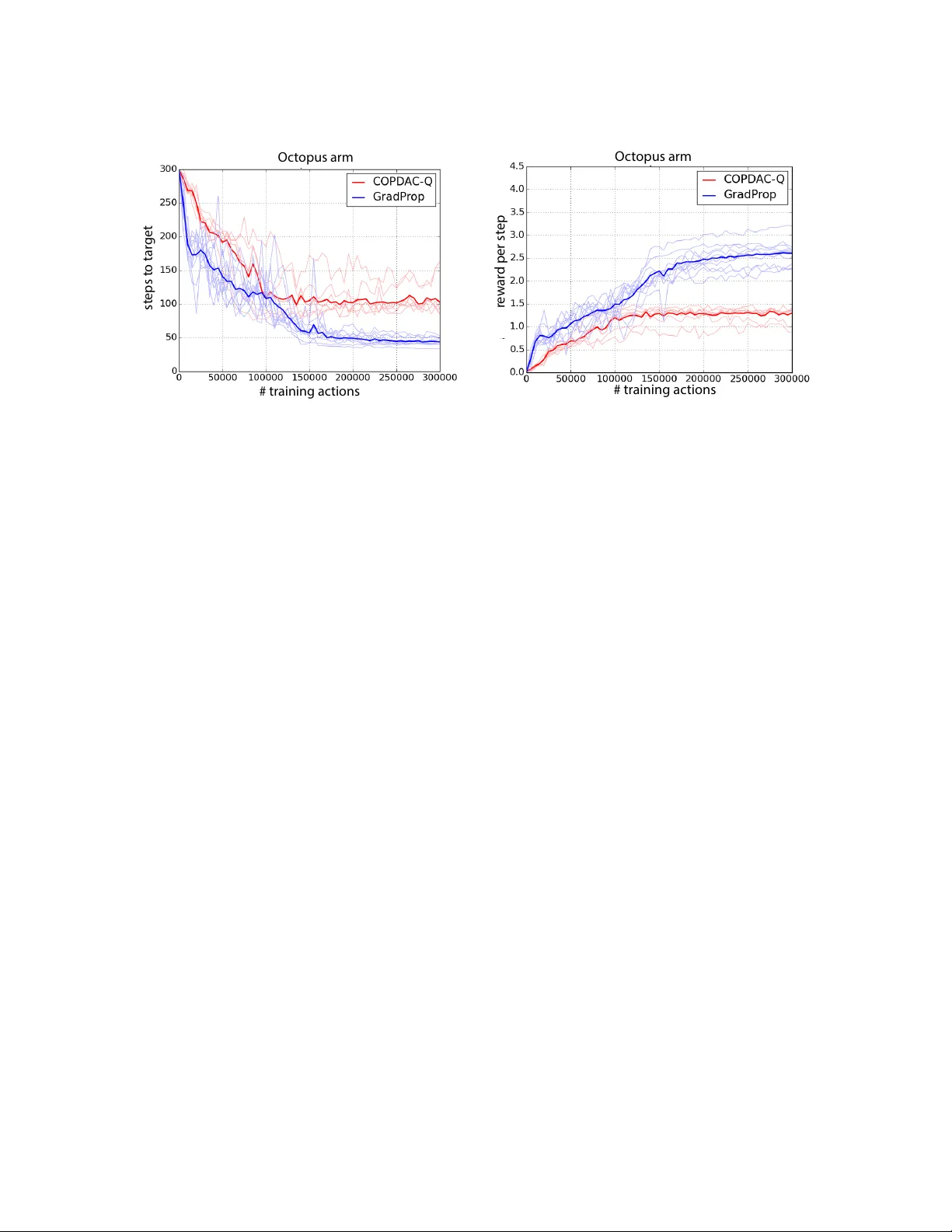
Compatible V alue Gradien ts for Reinforcemen t Learning of Con tin uous Deep P olicies Da vid Balduzzi da vid.balduzzi@vuw.ac.nz Scho ol of Mathematics and Statistics Victoria University of Wel lington Wel lington, New Ze aland Muhammad Ghifary muhammad.ghif ar y@ecs.vuw.ac.nz Scho ol of Engine ering and Computer Scienc e Victoria University of Wel lington Wel lington, New Ze aland Abstract This pap er prop oses GProp , a deep reinforcement learning algorithm for con tinuous poli- cies with compatible function appro ximation. The algorithm is based on t w o innov ations. Firstly , w e presen t a temp oral-difference based metho d for learning the gr adient of the v alue-function. Secondly , w e presen t the deviator-actor-critic (DA C) mo del, whic h com- prises three neural net works that estimate the v alue function, its gradient, and determine the actor’s p olicy resp ectively . W e ev aluate GProp on t wo c hallenging tasks: a contextual bandit problem constructed from nonparametric regression datasets that is designed to prob e the ability of reinforce- men t learning algorithms to accurately estimate gradients; and the o ctopus arm, a challeng- ing reinforcement learning benchmark. GProp is comp etitive with ful ly sup ervise d metho ds on the bandit task and achiev es the b est p erformance to date on the o ctopus arm. Keyw ords: p olicy gradient, reinforcement learning, deep learning, gradien t estimation, temp oral difference learning 1. In tro duction In reinforcemen t learning, an agent learns to maximize its discoun ted future rew ards ( Sutton and Barto , 1998 ). The structure of the en vironment is initially unknown, so the agent m ust b oth learn the rewards asso ciated with v arious action-sequence pairs and optimize its p olicy . A natural approac h is to tackle the subproblems separately via a critic and an actor ( Barto et al. , 1983 ; Konda and Tsitsiklis , 2000 ), where the critic estimates the v alue of differen t actions and the actor maximizes rew ards by follo wing the p olicy gradien t ( Sutton et al. , 1999 ; Peters and Schaal , 2006 ; Silv er et al. , 2014 ). P olicy gradien t metho ds hav e pro ven useful in settings with high-dimensional con tinuous action spaces, esp ecially when task- relev an t p olicy r epr esentations are at hand ( Deisenroth et al. , 2011 ; Levine et al. , 2015 ; W ahlstr¨ om et al. , 2015 ). W e tac kle the problem of learning actor (policy) and critic represen tations. In the sup ervised setting, represen tation or deep learning algorithms ha ve recently demonstrated remark able performance on a range of b enc hmark problems. Ho wev er, the problem of 1 Balduzzi and Ghif ar y learning features for reinforcement learning remains comparativ ely underdeveloped. The most dramatic recent success uses Q -learning ov er finite action spaces, and essentially build a neural net work critic ( Mnih et al. , 2015 ). Here, we consider c ontinuous action spaces, and dev elop an algorithm that simultaneously learns the v alue function and its gradien t, which it then uses to find the optimal p olicy . 1.1 Outline This paper presents V alue-Gradien t Backpropagation ( GProp ), a deep actor-critic algorithm for contin uous action spaces with compatible function appro ximation. Our starting p oint is the deterministic p olicy gradient and asso ciated compatibility conditions deriv ed in ( Silver et al. , 2014 ). Roughly sp eaking, the compatibilit y conditions are that C1. the critic appro ximate the gradien t of the v alue-function and C2. the approximation is closely related to the gradient of the policy . See Theorem 2 for details. W e identify and solv e t wo problems with prior w ork on p olicy gradien ts – relating to the t w o compatibilit y conditions: P1. T emp or al differ enc e metho ds do not dir e ctly estimate the gr adient of the value function. Instead, temp oral difference metho ds are applied to learn an appro ximation of the form Q v ( s ) + Q w ( s , a ), where Q v ( s ) estimates the v alue of a state, giv en the current p olicy , and Q w ( s , a ) estimates the advantage from deviating from the curren t p olicy ( Sutton et al. , 1999 ; P eters and Schaal , 2006 ; Deisenroth et al. , 2011 ; Silver et al. , 2014 ). Although the adv antage is related to the gradien t of the v alue function, it is not the same thing. P2. The r epr esentations use d for c omp atible appr oximation sc ale b ad ly on neur al networks. The second problem is that prior w ork has restricted to adv an tage functions constructed from a particular state-action representation, φ ( s , a ) = ∇ θ µ θ ( s )( a − µ θ ( s )), that de- p ends on the gradient of the p olicy . The represen tation is easy to handle for linear p olicies. Ho wev er, if the p olicy is a neural netw ork, then the standard state-action represen tation ties the critic too closely to the actor and dep ends on the internal struc- ture of the actor, Example 2 . As a result, w eigh t up dates cannot b e p erformed b y bac kpropagation, see section 5.5 . The pap er makes three nov el contributions. The first tw o contributions relate directly to problems P1 and P2. The third is a new task designed to test the accuracy of gradient estimates. Metho d to directly learn the gradien t of the v alue function. The first con tribution is to mo dify temp oral difference learning so that it directly estimates the gradient of the v alue-function. The gr adient p erturb ation trick , Lemma 3 , provides a wa y to sim ultaneously estimate b oth the v alue of a function at a p oin t and its gradient, b y p erturbing the function’s input with uncorrelated Gaussian noise. Plugging in a neural net w ork instead of a linear estimator extends the trick to the problem of learning a function and its gradient ov er the en tire state-action space. Moreov er, the trick com bines naturally with temp oral difference metho ds, Theorem 5 , and is therefore w ell-suited to applications in reinforcement learning. 2 Comp a tible V alue Gradients for Deep Reinf orcement Learning Deviator-Actor-Critic (D AC) mo del with compatible function approximation. The second contribution is to prop ose the Deviator-Actor-Critic (D AC) mo del, Definition 2 , consisting in three coupled neural netw orks and V alue-Gradien t Backpropagation ( GProp ), Algorithm 1 , which backpropagates three different signals to train the three net works. The main result, Theorem 6 , is that GProp has compatible function approximation when im- plemen ted on the DA C mo del when the neural net work consists in linear and rectilinear units. 1 The proof relies on decomposing the Actor-net work into individual units that are con- sidered as actors in their own right, based on ideas in ( Sriv as ta v a et al. , 2014 ; Balduzzi , 2015 ). It also suggests interesting connections to w ork on structural credit assignmen t in m ultiagent reinforcement learning ( Agogino and T umer , 2004 , 2008 ; HolmesP arker et al. , 2014 ). Con textual bandit task to prob e the accuracy of gradien t estimates. A third con tribution, that may b e of indep endent in terest, is a new contextual bandit setting de- signed to prob e the ability of reinforcement learning algorithms to estimate gradients. A sup ervised-to-con textual bandit transform was prop osed in ( Dud ´ ık et al. , 2014 ) as a method for turning classification datasets in to K -armed contextual bandit datasets. W e are interested in the c ontinuous setting in this pap er. W e therefore adapt their transform with a twist. The SARCOS and Barrett datasets from rob otics hav e features corresp onding to the p ositions, velocities and accelerations of sev en join ts and lab els corre- sp onding to their torques. There are 7 join ts in both cases, so the feature and lab el spaces are 21 and 7 dimensional resp ectiv ely . The datasets are traditionally used as regression b enc hmarks labeled SAR COS1 through SARCOS7 where the task is to predict the torque of a single join t – and similarly for Barrett. W e con vert the t wo datasets in to tw o contin uous contextual bandit tasks where the rew ard signal is the negative distance to the correct lab el 7-dimensional. The algorithm is th us “told” that the lab el lies on a sphere in a 7-dimensional space. The missing information required to pin do wn the label’s p osition is precisely the gradient. F or an algorithm to mak e predictions that are comp etitive with fully sup ervised metho ds, it is necessary to find extremely accurate gradien t estimates. Exp erimen ts. Section 6 ev aluates the performance of GProp on the contextual bandit problems describ ed ab ov e and on the challenging o ctopus arm task ( Engel et al. , 2005 ). W e sho w that GProp is able to simultaneously solv e sev en nonparametric regression prob- lems without observing any lab els – instead using the distance b etw een its actions and the correct labels. It turns out that GProp is competitive with recen t ful ly sup ervise d learning algorithms on the task. Finally , we ev aluate GProp on the o ctopus arm b enchmark, where it achiev es the b est performance reported to date. 1. The pro of also holds for maxp o oling, w eight-t ying and other features of convnets. A description of how closely related results extend to convnets is provided in ( Balduzzi , 2015 ). 3 Balduzzi and Ghif ar y 1.2 Related work An early reinforcement learning algorithm for neural netw orks is REINFORCE ( Williams , 1992 ). A disadv antage of REINFORCE is that the en tire netw ork is trained with a single scalar signal. Our proposal builds on ideas in tro duced with deep Q -learning ( Mnih et al. , 2015 ), such as repla y . Ho wev er, deep Q -learning is restricted to finite action spaces, whereas we are concerned with c ontinuous action spaces. P olicy gradients w ere introduced in ( Sutton et al. , 1999 ) and hav e b een used extensively ( Kak ade , 2001 ; Peters and Schaal , 2006 ; Deisenroth et al. , 2011 ). The deterministic p olicy gradien t was in tro duced in ( Silver et al. , 2014 ), whic h also prop osed the algorithm COPDAC-Q . The relationship betw een GProp and COPDAC-Q is discussed in detail in section 5.5 . An alternate approac h, based on the idea of backpropagating the gradien t of the v alue function, is dev elop ed in ( Jordan and Jacobs , 1990 ; Prokhoro v and W unsc h , 1997 ; W ang and Si , 2001 ; Hafner and Riedmiller , 2011 ; F airbank and Alonso , 2012 ; F airbank et al. , 2013 ). Unfortunately , these algorithms do not ha ve compatible function appro ximation in general, so there are no guaran tees on actor-critic in teractions. See section 5.5 for further discussion. The analysis used to pro v e compatible function appro ximation relies on decomp osing the Actor neural netw ork in to a collection of agents corresponding to the units in the netw ork. The relation b etw een GProp and the difference-based ob jective prop osed for m ultiagen t learning ( Agogino and T umer , 2008 ; HolmesPark er et al. , 2014 ) is discussed in section 5.4 . 1.3 Notation W e use b oldface to denote vectors, subscripts for time, and sup erscripts for individual units in a net work. Sets of parameters are capitalized (Θ, W , V ) when they refer to matrices or to the parameters of neural netw orks. 2. Deterministic Policy Gradien ts This section recalls previous w ork on policy gradien ts. The basic idea is to sim ultaneously train an actor and a critic. The critic learns an estimate of the v alue of different p olicies; the actor then follows the gradient of the v alue-function to find an optimal (or lo cally optimal) p olicy in terms of exp ected rewards. 2.1 The Policy Gradien t Theorem The environmen t is mo deled as a Mark o v Decision Process consisting of state space S ⊂ R m , action space A ⊂ R d , initial distribution p 1 ( s ) on states, stationary transition distribution p ( s t +1 | s t , a t ) and reward function r : S × A → R . A p olicy is a function µ θ : S → A from states to actions. W e will often add noise to p olicies, causing them to b e sto c hastic. In this case, the p olicy is a function µ θ : S → 4 A , where 4 A is the set of probabilit y distributions on actions. Let p t ( s → s 0 , µ ) denote the distribution on states s 0 at time t given p olicy µ and initial state s at t = 0 and let ρ µ ( s 0 ) = R S P ∞ t =0 γ t p 1 ( s ) p t ( s → s 0 , µ ) d s . Let r γ t = 4 Comp a tible V alue Gradients for Deep Reinf orcement Learning P ∞ τ = t γ τ − t r ( s τ , a τ ) b e the discoun ted future rew ard. Define the v alue of a state-action pair: Q µ θ ( s , a ) = E [ r γ 1 | S 1 = s , A 1 = a ; µ θ ] and v alue of a p olicy: J ( µ θ ) = E s ∼ ρ µ , a ∼ µ θ [ Q µ θ ( s , a )] . The aim is to find the p olicy θ ∗ := argmax θ J ( µ θ ) with maximal v alue. A natural ap- proac h is to follo w the gradient ( Sutton et al. , 1999 ), which in the deterministic case can b e computed explicitly as Theorem 1 (p olicy gradien t) Under r e asonable assumptions on the r e gularity of the Markov De cision Pr o c ess the p olicy gr adient c an b e c ompute d as ∇ θ J ( µ θ ) = E s ∼ ρ µ  ∇ θ µ θ ( s ) ∇ a Q µ ( s , a ) | a = µ θ ( s )  . Pro of See ( Silv er et al. , 2014 ). 2.2 Linear Compatible F unction Approximation Since the agent does not hav e direct access to the v alue function Q µ , it must instead learn an estimate Q w ≈ Q µ . A sufficient condition for when plugging an estimate Q w ( s , a ) in to the p olicy gradient ∇ θ J ( θ ) = E [ ∇ θ µ θ ( s ) ∇ a Q µ θ ( s , a ) | a = µ θ ( s ) ] yields an unbiased estimator w as first proposed in ( Sutton et al. , 1999 ). A sufficient condition in the deterministic setting is: Theorem 2 (compatible v alue function appro ximation) The value-estimate Q w ( s , a ) satisfies is c omp atible with the p olicy gr adient, that is ∇ θ J ( θ ) = E  ∇ θ µ θ ( s ) · ∇ a Q w ( s , a ) | a = µ θ ( s )  if the fol lowing c onditions hold: C1. Q w appr oximates the value gr adient: The weights le arne d by the appr oximate value function must satisfy w = argmin w 0 ` GE ( θ , w 0 ) , wher e ` GE ( θ , w ) := E     ∇ a Q w ( s , a ) | a = µ θ ( s ) − ∇ a Q µ ( s , a ) | a = µ θ ( s )    2  (1) is the me an-squar e differ enc e b etwe en the gr adient of the true value function Q µ and the appr oximation Q w . C2. Q w is p olicy-c omp atible: The gr adients of the value-function and the p olicy must satisfy ∇ a Q w ( s , a ) | a = µ θ ( s ) =  ∇ θ µ θ ( s ) , w  . (2) 5 Balduzzi and Ghif ar y Pro of See ( Silv er et al. , 2014 ). Ha ving stated the compatibilit y condition, it is w orth revisiting the problems that we prop ose to tackle in the paper. The first problem is to directly estimate the gradient of the v alue function, as required b y Eq. ( 1 ) in condition C1 . The standard approach used in the literature is to estimate the v alue function, or the closely related adv an tage function, using temp oral difference learning, and then compute the deriv ativ e of the estimate. The next section shows ho w the gradien t can be estimated directly . The second problem relates to the compatibility condition on p olicy and v alue gradien ts required b y Eq. ( 2 ) in condition C2 . The only function approximation satisfying C2 that has b een proposed is Example 1 (standard v alue function appro ximation) L et φ ( s ) b e an m -dimensional fe atur e r epr esentation on states and set φ ( s , a ) := ∇ θ µ θ ( s ) ·  a − µ θ ( s )  . Then the value function appr oximation Q v , w ( s , a ) = h φ ( s , a ) , w i | {z } advantage function +  φ ( s ) , v  = ( a − µ θ ( s )) | · ∇ θ µ θ ( s ) | · w + φ ( s ) | · v . satisfies c ondition C2 of The or em 2 . The approximation in Example 1 encounters serious problems when applied to de ep p olicies, see discussion in section 5.5 . 3. Learning V alue Gradients In this section, w e tackle the first problem by mo difying temp oral-difference (TD) learning so that it directly estimates the gradien t of the v alue function. First, we developed a new approac h to estimating the gradient of a black-box function at a p oint, based on p erturbing the function with gaussian noise. It turns out that the approac h extends easily to learning the gradient of a blac k-box function across its en tire domain. Moreov er, it is easy to com bine with neural net w orks and temporal difference learning. 3.1 Estimating the gradien t of an unknown function at a p oin t Gradien t estimates hav e b een intensiv ely studied in bandit problems, where rewards (or losses) are observed but lab els are not. Thus, in con trast to sup ervised learning where it is p ossible to compute the gradient of the loss, in bandit problems the gradient must b e estimated. More formally , consider the follo wing setup. Definition 1 (zeroth-order blac k-b ox) A function f : R d → R is a zer oth-or der black-b ox if it c an only b e querie d for zeroth- order information. That is, User c an r e quest the value f ( x ) of f at any p oint x ∈ R d , but c annot r e quest the gr adient of the function. We use the shorthand blac k-b o x in what fol lows. 6 Comp a tible V alue Gradients for Deep Reinf orcement Learning The black-box mo del for optimization w as introduced in ( Nemirovski and Y udin , 1983 ), see ( Raginsky and Rakhlin , 2011 ) for a recen t exp osition. In those pap ers, a black-box consists in a first-or der or acle that can pro vide b oth zeroth-order information (the v alue of the function) and first-order information (the gradien t or subgradient of the function). Remark 1 (rew ard function is a blac k-b ox; v alue function is not) The r ewar d function r ( s , a ) is a black b ox sinc e Natur e do es not pr ovide gr adient informa- tion. The value function Q µ θ ( s , a ) = E [ r γ 1 | S 1 = s , A 1 = a ; µ θ ] is not ev en a black-b ox: it c annot b e querie d dir e ctly sinc e it is define d as the exp e cte d disc ounte d future r ewar d. It is for this r e ason the gr adient p erturb ation trick must b e c ombine d with temp or al differ enc e le arning, se e se ction 3.4 . An imp ortant insight is that the gradien t of an unknown function at a sp ecific p oint can b e estimated b y p erturbing its input ( Flaxman et al. , 2005 ). F or example, for small δ > 0 the gradient of f : R d → R is approximately ∇ f ( x ) | x = µ ≈ d · E u [ f ( µ + δ u ) δ u ] where the exp ectation is o v er vectors sampled uniformly from the unit sphere. The following lemma pro vides a simple metho d for estimating the gradient of a function at a p oint based on Gaussian perturbations: Lemma 3 (gradien t p erturbation tric k) The gr adient of differ entiable f : R d → R at µ ∈ R d is ∇ x f ( x ) | x = µ = lim σ 2 → 0 argmin w ∈ R d  min b ∈ R E  ∼ N ( 0 ,σ 2 · I d )   f ( µ +  ) − h w ,  i − b  2  . (3) Pro of By taking sufficiently small v ariance, we can assume that f is lo cally linear. Setting b = f ( µ ) yields a line through the origin. It therefore suffices to consider the special case f ( x ) = h v , x i . Setting w ∗ = argmin w ∈ R d E  ∼ N ( 0 ,σ 2 · I d )  1 2  h w ,  i − h v ,  i  2  , w e are required to sho w that w ∗ = v . The problem is con vex, so setting the gradient to zero requires to solv e 0 = E  h w − v ,  i ·   , which reduces to solving the set of linear equations d X i =1 ( w i − v i ) E [  i  j ] = ( w j − v j ) E [(  j ) 2 ] = ( w j − v j ) · σ 2 = 0 for all j . The first equalit y holds since E [  i  j ] = 0. It follows immediately that w ∗ = v . 3.2 Learning gradients across a range The solution to the optimization problem in Eq. ( 3 ) is the gradient ∇ f ( x ) of f at a particular µ ∈ R d . The next step is to learn a function G W : R d → R d that appro ximates the gradient across a range of v alues. 7 Balduzzi and Ghif ar y More precisely , given a sample { x i } n i =1 ∼ P X of p oints, w e aim to find W ∗ := argmin W n X i =1 h   ∇ f ( x i ) − G W ( x i )   2 i . The next lemma considers the case where Q v and G W are linear estimates, of the form Q v ( x ) := h φ ( x ) , v i , and G W ( x ) = W · ψ ( x ) for fixed representations φ : X → R m and ψ : X → R n . Lemma 4 (gradien t learning) L et f : R d → R b e a differ entiable function. Supp ose that φ : X → R m and ψ : X → R n ar e r epr esentations such that ther e exists an m -ve ctor v ∗ and a ( d × n ) -matrix W ∗ satisfying f ( x ) = h φ ( x ) , v ∗ i and ∇ f = W ∗ · ψ ( x ) for al l x in the sample. If we define loss function ` ( W , V , x , σ ) = E    f ( x +  ) − h G W ( x ) ,  i − Q V ( x )  2  . then W ∗ = lim σ 2 → 0 argmin W min V E x ∼ ˆ P  ` ( W , V , x , σ )  . Pro of F ollows from Lemma 3 . In short, the lemma reduces gradient estimation to a simple optimization problem given a go o d enough r epr esentation . Jumping ahead slightly to section 4 , we ensure that our mo del has go o d enough representations b y constructing t w o neural netw orks to learn them. The first neural net work, Q V : R d → R , learns an approximation to f ( x ) that plays the role of the baseline b . The second neural netw ork, G W : R d → R d learns an appro ximation to the gradien t. 3.3 T emporal difference learning Recall that Q µ ( s , a ) is the exp ected v alue of a state-action pair given p olicy µ . It is never observ ed directly , since it is computed by discounting o v er future rew ards. TD-learning is a p opular approach to es timating Q µ through dynamic programming ( Sutton and Barto , 1998 ). W e quickly review TD-learning. Let φ : S × A → R m b e a fixed representation. The goal is to find a v alue-estimate Q v ( s , a ) := h φ ( s , a ) , v i , where v is an m -dimensional vector, that is as close as p ossible to the true v alue function. If the v alue-function were known, we could simply minimize the mean-square error with resp ect to v : ` M S E ( v ) = E ( s , a ) ∼ ( ρ µ , µ )   Q µ ( s , a ) − Q v ( s , a )  2  . 8 Comp a tible V alue Gradients for Deep Reinf orcement Learning Unfortunately , it is impossible to minimize the mean-square error directly , since the v alue- function is the exp ected discoun ted future reward, rather than the rew ard. That is, the v alue function is not pro vided explicitly b y the environmen t – not even as a black-box. The Bellman error is therefore used a substitute for the mean-square error: ` B E ( v ) = E ( s , a ) ∼ ( ρ µ , µ ) h TD-error, δ z }| { r ( s , a ) + γ Q v ( s 0 , µ ( s 0 )) | {z } ≈ Q µ ( s , a ) − Q v ( s , a )  2 i where s 0 is the state subsequen t to s . Let δ t = r t − Q v ( s t , a t ) + γ Q v ( s t +1 , µ θ ( s t +1 )) b e the TD-error. TD-learning up dates v according to v t +1 ← v t + η t · δ t · ∇ v Q v ( s t , a t ) = v t + η t · δ t · φ ( s , a ) , (4) where η t is a sequence of learning rates. The conv ergence prop erties of TD-learning and related algorithms hav e b een studied extensively , see ( Tsitsiklis and Roy , 1997 ; Dann et al. , 2014 ). 3.4 T emporal difference gradien t (TDG) learning Finally , we apply temp oral difference metho ds to estimate the gr adient 2 of the v alue func- tion, as required b y condition C1 of Theorem 2 . W e are in terested in gradien t approxima- tions of the form Q W ( s , a ,  ) := h G W ( s , a ) ,  i = h W · ψ ( s , a ) ,  i , where ψ : S × A → R n and W is a ( d × n )-dimensional matrix. The goal is to find W ∗ suc h that G W ∗ ( s , a ) ≈ ∇  Q µ ( s , a ,  ) |  = 0 = ∇ a Q µ ( s , a ) | a = µ θ ( s ) for all sampled state-action pairs. It is conv enient to in tro duce notation Q µ ( s , a ,  ) := Q µ ( s , a +  ) and shorthand ˜ s := ( s , µ Θ ( s )). Then, analogously to the mean-square, define the perturb ed gradien t error: ` P GE ( v , W ; σ 2 ) = E s ∼ ρ µ E    Q µ ( ˜ s ,  ) −  G W ( ˜ s ) ,   − Q v ( ˜ s )  2  , Giv en a go o d enough represen tation, Lemma 4 guaran tees that minimizing the p erturb ed gradien t error yields the gradient of the v alue function. Unfortunately , as discussed ab o ve, the v alue function cannot b e queried directly . W e therefore in tro duce the Bellman gradien t error as a pro xy ` B GE ( v , W ; σ 2 ) = E s ∼ ρ µ E  h TDG-error, ξ z }| { r ( ˜ s ,  ) + γ Q v  ˜ s 0 ) | {z } ≈ Q µ ( ˜ s ,  ) −  G W ( ˜ s ) ,   − Q v ( ˜ s )  2 i . 2. Residual gradient (RG) and gradient temporal difference (GTD) methods w ere introduced in ( Baird , 1995 ; Sutton et al. , 2009a , b ). The similar names ma y be confusing. RG and GTD metho ds are TD metho ds derived from gradient descen t. In contrast, we develop a TD-based approach to le arning gr a- dients . The t wo approac hes are thus complemen tary and straightforw ard to com bine. Ho wev er, in this pap er we restrict to extending v anilla TD to learning gradients. 9 Balduzzi and Ghif ar y Set the TDG-error as ξ t = r ( ˜ s t  ) + γ Q v ( ˜ s t +1 ) − h G W ( ˜ s t ) ,  i − Q v ( ˜ s t ) and, analogously to Eq. ( 4 ), define the TDG-up dates v t +1 ← v t + η t · ξ t · ∇ v Q v ( ˜ s t ) = v t + η t · ξ t · φ ( ˜ s t ) W t +1 ← W t + η t · ξ t · ∇ W Q W ( ˜ s t ) = W t + η t · ξ t ·  ⊗ ψ ( ˜ s t ) , where  ⊗ ψ ( ˜ s t ) is the ( d × n ) matrix giv en b y the outer product. W e refer to ξ ·  as the p erturb ed TDG-error . The following extension the or em allows us to imp ort guarantees from temp oral-difference learning to temporal-difference gradient learning. Theorem 5 (zeroth to first-order extension) Guar ante es on TD-le arning extend to TDG-le arning. The idea is to reform ulate TDG-learning as TD-learning, with a sligh tly differen t rew ard function and function approximation. Since the function approximation is still linear, an y guaran tees on con vergence for TD-learning transfered automatically to TDG-learning. Pro of First, we incorp orate  in to the state-action pair. Define ˜ r ( s , a ,  ) := r ( s , a +  ) and ˜ ψ ( s , a ,  ) =  ⊗ ψ ( s , a ) . Second, we define a dot pro duct on matrices of equal size b y flattening them do wn to v ectors. More precisely , giv en tw o matrices A and B of the same dimension ( m × n ), define the dot-pro duct h A , B i = P m,n i,j =1 A ij B ij . It is easy to see that G W ( s , a ) := h W · ψ ( s , a ) ,  i = h ˜ ψ ( s , a ,  ) , W i . The TDG-error can then b e rewritten as ξ t = ˜ r ( s , a ,  ) + γ Q v , W ( s 0 , a 0 ,  0 ) − Q v , W ( s , a ,  ) where Q v , W ( s , a ,  ) = h φ ( s , a ) , v i + h ˜ ψ ( s , a ,  ) , W i is a linear function approximation. If w e are in a setting where TD-learning is guaranteed to con v erge to the v alue-function, it follo ws that TDG-learning is also guaran teed to con verge – since it is simply a differ- en t linear appro ximation. Thus, Q µ ( ˜ s ,  ) ≈ Q v ( ˜ s ) + G W ( ˜ s ,  ) and the result follows by Lemma 4 . 4. Algorithm: V alue-Gradien t Backpropagation This section presen ts our mo del, whic h consists of three coupled neural net w orks that learn to estimate the v alue function, its gradient, and the optimal policy respectively . 10 Comp a tible V alue Gradients for Deep Reinf orcement Learning Definition 2 (deviator-actor-critic) The deviator-actor-critic (DA C) mo del c onsists in thr e e neur al networks: • actor-network with p olicy µ Θ : S → A ⊂ R d ; • critic-network , Q V : S × A → R , that estimates the value function; and • deviator-network , G W : S × A → R d , that estimates the gr adient of the value function. Gaussian noise is adde d to the p olicy during tr aining r esulting in actions a = µ Θ ( s ) +  wher e  ∼ N ( 0 , σ 2 · I d ) . The outputs of the critic and deviator ar e c ombine d as Q W , V  s , µ Θ ( s ) ,   = Q V  s , µ Θ ( s )  + D G W  s , µ Θ ( s )  ,  E . The Gaussian noise pla ys t wo roles. Firstly , it controls the explore/exploit tradeoff b y con trolling the extent to whic h Actor deviates from its current optimal p olicy . Secondly , it con trols the “resolution” at which Deviator estimates the gradien t. The three net works are trained by bac kpropagating three differen t signals. Critic, De- viator and Actor backpropagate the TDG-error, the p erturb ed TDG-error, and Deviator’s gradien t estimate resp ectiv ely; see Algorithm 1 . An explicit description of the weigh t up- dates of individual units is provided in App endix A . Deviator estimates the gradien t of the v alue-function with resp ect to deviations  fr om the curr ent p olicy . Bac kpropagating the gradien t through Actor allows to estimate the influence of Actor-parameters on the v alue function as a function of their effect on the p olicy . Algorithm 1: Value-Gradient Backpropagation (GProp) . for r ounds t = 1 , 2 , . . . , T do Net work gets state s t , resp onds a t = µ Θ t ( s t ) +  , gets rew ard r t Let ˜ s := ( s , µ Θ ( s )). ξ t ← − r t + γ Q V t ( ˜ s t +1 ) − Q V t ( ˜ s t ) −  G W t ( ˜ s t ) ,   // compute TDG-error Θ t +1 ← − Θ t + η A t · ∇ Θ µ Θ t ( s t ) · G W t  ˜ s t  // backpropagate G W V t +1 ← − V t + η C t · ξ t · ∇ V Q V t ( ˜ s t ) // backpropagate ξ W t +1 ← − W t + η D t · ξ t · ∇ W G W t ( ˜ s t ) ·  // backpropagate ξ ·  Critic and Deviator learn representations suited to estimating the v alue function and its gradien t respectively . Note that even though the gradien t is a linear function at a p oint , it can b e a highly nonlinear function in general. Similarly , Actor learns a p olicy represen tation. W e set the learning rates of Critic and Deviator to b e equal ( η C t = η D t ) in the exp erimen ts in section 6 . Ho wev er, the p erturbation  has the effect of slowing do wn and stabilizing Deviator up dates: Remark 2 (stabilit y) The magnitude of Deviator’s weight up dates dep end on  ∼ N ( 0 , σ 2 · I d ) sinc e they ar e c ompute d by b ackpr op agating the p erturb e d TDG-err or ξ ·  . Thus as σ 2 → 0 , Deviator’s le arning r ate essential ly tends to zer o. In gener al, Deviator le arns mor e slow ly than Critic. 11 Balduzzi and Ghif ar y This has a stabilizing effe ct on the p olicy sinc e A ctor is insulate d fr om Critic – its weight up dates only dep end (dir e ctly) on the output of Deviator. 5. Analysis: Deep Compatible F unction Appro ximation Our main result is that the deviator’s v alue gradient is compatible with the policy gradien t of each unit in the actor-net w ork – considered as an actor in its o wn righ t: Theorem 6 (deep compatible function appro ximation) Supp ose that al l units ar e r e ctiline ar or line ar. Then for e ach A ctor-unit in the A ctor- network ther e exists a r ep ar ametrization of the value-gr adient appr oximator, G W , that sat- isfies the c omp atibility c onditions in The or em 2 . The actor-net work is thus a collection of interdependent agents that individually fol- lo w the correc t p olicy gradients. The exp eriments b elo w show that they also collectiv ely con verge on useful b ehaviors. Ov erview of the pro of. The next few subsections pro ve Theorem 6 . W e pro vide a brief o verview b efore diving into the details. Guaran tees for temp oral difference learning and p olicy gradients are t ypically based on the assumption that the v alue-function approximation is a line ar function of the learned parameters. How ev er, we are in terested in the case where Actor, Critic and Deviator are all neural net w orks, and are therefore highly nonlinear functions of their parameters. The goal is thus to relate the representations learned b y neural netw orks to the prior w ork on linear function appro ximations. T o do so, w e build on the following observ ation, implicit in ( Sriv asta v a et al. , 2014 ): Remark 3 (activ e submo dels) A neur al network of n line ar and r e ctiline ar units c an b e c onsider e d as a set of 2 n submo dels, c orr esp onding to differ ent subsets of units. The active submo del at time t c onsists in the active units (that is, the line ar units and the r e ctifiers that do not output 0). The active submo del has two imp ortant pr op erties: • it is a linear function fr om inputs to outputs, sinc e r e ctifiers ar e line ar when active, and • at e ach time step, le arning only o c curs over the active submo dels, sinc e only active units up date their weights. The feedforward sw eep of a rectifier netw ork can th us b e disen tangled into t wo steps ( Bal- duzzi , 2015 ). The first step, whic h is highly nonlinear, applies a gating op eration t hat selects the active submodel – by rendering v arious units inactiv e. The second step computes the output of the neural net w ork via matrix m ultiplication. It is important to emphasize that although the activ e submodel is a linear function from inputs to outputs, it is not a linear function of the w eights. The strategy of the pro of is to decomp ose the Actor-netw ork in an interacting collection of agen ts, referred to as Actor-units. That is, w e mo del eac h unit in the Actor-net w ork as 12 Comp a tible V alue Gradients for Deep Reinf orcement Learning an Actor in its own right that. On each time step that an Actor-unit is active, it interacts with the Deviator-submo del corresp onding to the curren t activ e submo del of the Deviator- net work. The pro of sho ws that eac h Actor-unit has compatible function approximation. 5.1 Error backpropagation on rectilinear neural net works First, w e recall some basic facts ab out backpropagation in the case of r e ctiline ar units. Recen t work has sho wn that replacing sigmoid functions with rectifiers S ( x ) = max(0 , x ) impro ves the performance of neural net works ( Nair and Hin ton , 2010 ; Glorot et al. , 2011 ; Zeiler et al. , 2013 ; Dahl et al. , 2013 ). Let us establish some notation. The output of a rectifier with w eigh t vector w is S w ( x ) := S ( h w , x i ) := max(0 , h w , x i ) . The rectifier is activ e if h w , x i > 0. W e use rectifiers b ecause they p erform w ell in prac- tice and hav e the nice prop ert y that units are line ar when they are active. The rectifier subgradien t is the indicator function 1 ( x ) := ∇ S ( x ) = ( 1 x > 0 0 else . Consider a neural net work of n units, eac h equipp ed with a weigh t vector w j ∈ H j ⊂ R d j . Hidden units are rectifiers; output units are linear. There are n units in total. It is con venien t to combine all the weigh t vectors into a single ob ject; let W ⊂ H = Q n j =1 H j ⊂ R N where N = P n j =1 d j . The net work is a function F W : R m → R d : x in 7→ F W ( x in ) =: x out . The net w ork has error function E ( x out , y ) with gradien t g = ∇ x out E . Let x j denote the output of unit j and φ j ( x in ) = ( x i ) { i : i → j } denote its input, so that x j = S ( h w j , φ j ( x in ) i . Note that φ j dep ends on W (sp ecifically , the w eights of lo wer units) but this is supressed from the notation. Definition 3 (influence) The influence of unit j on unit k at time t is π j,k t := ∂ x k t ∂ x j t ( Balduzzi et al. , 2015 ). The influenc e of unit j on the output layer is the ve ctor π j t =  π j,k t  k ∈ out . The following lemma summarizes an analysis of the feedforw ard and feedbac k sweep of neural nets. Lemma 7 (structure of neural net work gradien ts) The fol lowing pr op erties hold a. Influenc e. A p ath is active at time t if al l units on the p ath ar e firing. The influenc e of j on k is the sum of pr o ducts of weights over al l active p aths fr om j to k : π j,k t = X { α | j → α } w j,α 1 α t   X { β | α → β } w α,β 1 β t   · · · X { ω | ω → k } w ω ,k 1 k t     . wher e α, β , . . . , ω r efer to units along the p ath fr om j to k . 13 Balduzzi and Ghif ar y b. Output de c omp osition. The output of a neur al network de c omp oses, r elative to the output of unit j , as F W ( x in ) = π j · x j + π − j · x in , wher e π − j is the ( m × d ) -matrix whose ( ik ) th entry is the sum over al l active p aths fr om input unit i to output unit k that do not interse ct unit j . c. Output gr adient. Fix an input x in ∈ R m and c onsider the network as a function fr om p ar ameters to outputs F • ( x in ) : H → R d : W 7→ F W ( x in ) whose gr adient is an ( N × d ) -matrix. The ( ij ) th -entry of the gr adient is the input to the unit times its influenc e:  ∇ W F W ( x in )  ij = ( φ ij ( x in ) · π j if unit j is active 0 else. d. Backpr op agate d err or. Fix x in ∈ R m and c onsider the function E ( W ) = E ( F • ( x in ) , y ) : H → R : W 7→ E ( F W ( x in ) , y ) . L et g = ∇ x out E ( x out , y ) . The gr adient of the err or function is ( ∇ W E ) ij = D g ,  ∇ W F W ( x in )  ij E = g | ·  ∇ W F W ( x in )  ij = δ j · φ j ( x in ) wher e the b ackpr op agate d err or signal δ j r e c eive d by unit j de c omp oses as δ j =  g , π j  . Pro of Direct computation. The lemma holds generically for netw orks of rectifier and linear units. W e apply it to actor, critic and deviator net works b elo w. 5.2 A minimal D AC mo del This subsection pro v es condition C1 of compatible function approximation for a minimal, linear Deviator-Actor-Critic mo del. The next subsection sho ws how the minimal model arises at the lev el of Actor-units. Definition 4 (minimal mo del) The minimal mo del of a Deviator-A ctor-Critic c onsists in an A ctor with line ar p olicy µ θ ( s ) = h θ , φ ( s ) i +  , wher e θ is an m -ve ctor and  is a noisy sc alar. The Critic and Deviator to gether output: Q w, v ( s , µ θ ( s ) ,  ) = Q v ( s ) + G w ( µ θ ( s ) ,  ) = h φ ( s ) , v i | {z } Critic + µ θ ( s ) · h , w i | {z } Deviator , wher e v is an m -ve ctor, w is a sc alar, and h , w i is simply sc alar multiplic ation. 14 Comp a tible V alue Gradients for Deep Reinf orcement Learning The Critic in the minimal mo del is standard. Ho wev er, the Deviator has b een reduced to almost nothing: it learns a single scalar parameter, w , that is used to train the actor. The minimal model is th us to o simple to b e muc h use as a standalone algorithm. Lemma 8 (compatible function approximation for the minimal mo del) Ther e exists a r ep ar ametrization of the gr adient estimate of the minimal mo del G ˜ w ( s ,  ) = G w ( µ θ ( s ) ,  ) such that c omp atibility c ondition C1 in The or em 2 is satisife d: ∇  G ˜ w ( s ,  ) = h∇ θ µ θ ( s ) , ˜ w i . Pro of Let ˜ w := w · θ | and construct G ˜ w ( s ,  ) := h ˜ w · φ ( s ) ,  i . Clearly , G ˜ w ( s ,  ) = h w · θ | · φ ( s ) ,  i = µ θ ( s ) · h w ,  i = G w ( µ θ ( s ) ,  ) . Observ e that ∇  G ˜ w ( s ,  ) = w · µ θ ( s ) and that, similarly ,  ∇ θ µ θ ( s ) , ˜ w  = w · µ θ ( s ) as required. 5.3 Pro of of Theorem 6 The pro of pro ceeds b y showing that the compatibilit y conditions in Theorem 2 hold for eac h Actor-unit. The key step is to relate the Actor-units to the minimal mo del in tro duced ab o ve. Lemma 9 (reduction to minimal mo del) A ctor-units in a DA C neur al network ar e e quivalent to minimal mo del A ctors. Pro of Let π j t denote the influence of unit j on the output lay er of the Actor-net w ork at time t . When unit j is activ e, Lemma 7 ab implies we can write µ Θ t ( s t ) = π j t · h θ j t , φ j t ( s t ) i + µ Θ − j t ( s t ), where µ Θ − j t ( s t ) is the sum ov er all activ e paths from the input to the output of the Actor-netw ork that do not in tersect unit j . F ollo wing Remark 3 , the activ e subnetw ork of the Deviator-netw ork at time t is a linear transform which, b y abuse of notation, we denote by W 0 t . Com bine the last tw o p oin ts to obtain G W t ( ˜ s t ) = W 0 t ·  π j t · h θ j , φ j t ( s t ) i + µ Θ − j t ( s t )  = ( W 0 t · π j t ) · h θ j , φ j t ( s t ) i + terms that can b e omitted . Observ e that ( W 0 t · π j t ) is a d -v ector. W e hav e therefore reduced Actor-unit j ’s in teraction with the Deviator-net w ork to d copies of the minimal mo del. Theorem 6 follo ws from combining the ab ov e Lemmas. 15 Balduzzi and Ghif ar y Pro of Compatibilit y condition C1 follows from Lemmas 8 and 9 . Compatibilit y condition C2 holds since the Critic and Deviator minimize the Bellman gradient error with resp ect to W and V which also, implicitly , minimizes the Bellman gradient error with resp ect to the corresp onding reparametrized ˜ w ’s for eac h Actor-unit. Theorem 6 sho ws that each Actor-unit satisfies the conditions for compatible function appro ximation and so follows the correct gradient when p erforming weigh t up dates. 5.4 Structural credit assignmen t for m ultiagen t learning It is interesting to relate our approach to the literature on multiagen t reinforcement learning ( Guestrin et al. , 2002 ; Agogino and T umer , 2004 , 2008 ). In particular, ( HolmesP arker et al. , 2014 ) consider the structur al cr e dit assignment pr oblem within p opulations of interacting agen ts: How to reward individual agen ts in a p opulation for rewards based on their collectiv e b eha vior? They prop ose to train agents within populations with a differ enc e-b ase d obje ctive of the form D j = Q ( z ) − Q ( z − j , c j ) (5) where Q is the ob jectiv e function to b e maximized; z j and z − j are the system v ariables that are and are not under the control of agent j resp ective, and c j is a fixed counterfactual action. In our setting, the gradient used by Actor-unit j to up date its weigh ts can b e describ ed explicitly: Lemma 10 (lo cal p olicy gradien ts) A ctor-unit j fol lows p olicy gr adient ∇ J [ µ θ j ] = E  ∇ θ j µ θ j ( s ) ·  π j , G W ( ˜ s )   , wher e h π j , G W ( ˜ s )  ≈ D π j Q µ ( ˜ s ) is Deviator’s estimate of the dir e ctional derivative of the value function in the dir e ction of A ctor-unit j ’s influenc e. Pro of F ollows from Lemma 7 b. Notice that ∇ z j Q = ∇ z j D j in Eq. ( 5 ). It follo ws that training the Actor-net w ork via GProp causes the Actor-units to optimize the difference-based ob jective – without requiring to compute the difference explicitly . Although the topic is b ey ond the scope of the current pap er, it is w orth exploring ho w suitably adapted v arian ts of bac kpropagation can b e applied to the reinforcemen t learning problems in the multiagen t setting. 5.5 Comparison with related w ork Comparison with COPDAC-Q . Extending the standard v alue function approximation in Example 1 to the setting where Actor is a neural netw ork yields the following representation, whic h is used in ( Silver et al. , 2014 ) when applying COPDAC-Q to the o ctopus arm task: 16 Comp a tible V alue Gradients for Deep Reinf orcement Learning Example 2 (extension of standard v alue appro ximation to neural netw orks) L et µ Θ : S → A and Q V : S → R b e an A ctor and Critic neur al network r esp e ctively. Supp ose the A ctor-network has N p ar ameters (i.e. the total numb er of entries in Θ ). It fol lows that the Jac obian ∇ Θ µ Θ ( s ) is an ( N × d ) -matrix. The value function appr oximation is then Q V , W ( s , a ) = ( a − µ Θ ( s )) | · ∇ Θ µ Θ ( s ) | · w | {z } advantage function + Q V ( s ) | {z } Critic . wher e w is an N -ve ctor. W eigh t up dates under COPDAC-Q , with the function appro ximation abov e, are therefore as describ ed in Algorithm 2 . Algorithm 2: Compatible Deterministic Actor-Critic (COPDAC-Q) . for r ounds t = 1 , 2 , . . . , T do Net work gets state s t , resp onds a t = µ Θ t ( s t ) +  where  ∼ N ( 0 , σ 2 · I d ), gets rew ard r t δ t ← − r t + γ Q V t ( s t +1 ) − Q V t ( s t ) − h∇ Θ µ Θ t ( s t ) ·  , w t i Θ t +1 ← − Θ t + η A t · ∇ Θ µ Θ t ( s t ) · ∇ Θ µ Θ t ( s t ) | · w t V t +1 ← − V t + η C t · δ t · ∇ V Q V t ( s t ) w t +1 ← − w t + η C t · δ t · ∇ Θ µ Θ t ( s t ) ·  Let us compare GProp with COPDAC-Q , considering the three up dates in turn: • A ctor up dates. Under GProp , the Actor backpropagates the v alue-gradient estimate. In con trast under COPDAC-Q the Actor p erforms a complicated up date that combines the p olicy gradien t ∇ Θ µ ( s ) with the adv an tage function’s weigh ts – and differs substantiv ely from backprop. • Deviator / advantage-function up dates. Under GProp , the Deviator backpropagates the p erturb ed TDG-error. In contrast, COPDAC-Q uses the gradien t of the A ctor to up date the weigh t vector w of the adv an- tage function. By Lemma 7 d, bac kprop takes the form g | · ∇ Θ µ Θ ( s ) where g is a d -v ector. In con trast, the adv an tage function requires computing ∇ Θ µ Θ ( s ) | · w , where w is an N -vector. Although the tw o formulae appear similarly sup erficially , they carry very differen t computational costs. The first consequence is that the parameters of w m ust exactly line up with those of the policy . The second consequence is that, by Lemma 7 c, the adv an tage function requires access to ( ∇ Θ µ Θ ( s )) ij = ( φ ij ( s ) · π j if unit j is active 0 else , where φ ij ( s ) is the input from unit i to unit j . Th us, the adv an tage function requires access to the input φ j ( s ) and the influence π j of every unit in the Actor-net w ork. 17 Balduzzi and Ghif ar y • Critic up dates. The critic up dates for the tw o algorithms are essen tially iden tical, with the TD-error replaced with the TDG-error. In short, the approximation in Example 2 that is used by COPDAC-Q is thus not w ell- adapted to deep learning. The main reason is that learning the adv antage function requires coupling the v ector w with the parameters Θ of the actor. Comparison with computing the gradien t of the v alue-function appro ximation. P erhaps the most natural approach to estimating the gradien t is to simply estimate the v alue function, and then use its gradien t as an estimate of the deriv ativ e ( Jordan and Jacobs , 1990 ; Prokhoro v and W unsc h , 1997 ; W ang and Si , 2001 ; Hafner and Riedmiller , 2011 ; F airbank and Alonso , 2012 ; F airbank et al. , 2013 ). The main problem with this approach is that, to date, it has not b een sho w that the resulting up dates of the Critic and the Actor are compatible. There are also no guaran tees that the gradient of the Critic will be a go o d approximation to the gradient of the v alue function – although it is intuitiv ely plausible. The problem b ecomes particularly sev ere when the v alue-function is estimated via a neural netw ork that uses activ ation functions that are not smo oth suc h as rectifers. Rectifiers are b ecoming increasingly p opular due to their sup erior empirical p erformance ( Nair and Hin ton , 2010 ; Glorot et al. , 2011 ; Zeiler et al. , 2013 ; Dahl et al. , 2013 ). 6. Exp erimen ts W e ev aluate GProp on three tasks: t wo highly nonlinear contextual bandit tasks constructed from b enchmark datasets for nonparametric regression, and the octopus arm. W e do not ev aluate GProp on other standard reinforcemen t learning b enchmarks such as Mountain Car, P endulum or Puddle W orld, since these can already b e handled by line ar actor-critic algorithms. The contribution of GProp is the ability to learn representations suited to nonlinear problems. Cloning and repla y . T emp oral difference learning can b e unstable when run o ver a neural net work. A recen t innov ation in tro duced in ( Mnih et al. , 2015 ) that stabilizes TD- learning is to clone a separate netw ork Q ˜ V to compute the targets r t + γ Q ˜ V ( ˜ s t +1 ). The parameters of the cloned netw ork are up dated perio dically . W e implemen t a similar mo dification of the TDG-error in Algorithm 1 . W e also use exp erience repla y ( Mnih et al. , 2015 ). GProp is well-suited to replay , since the critic and deviator can learn v alues and gradients o ver the full range of previously observ ed state- action pairs offline. Cloning and repla y w ere also applied to COPDAC-Q . Both algorithms w ere implemen ted in Theano ( Bergstra et al. , 2010 ; Bastien et al. , 2012 ). 6.1 Con textual Bandit T asks The goal of the contextual bandit tasks is to prob e the ability of reinforcement learning algorithms to accurately estimate gradien ts. The experimental setting ma y th us b e of indep enden t in terest. 18 Comp a tible V alue Gradients for Deep Reinf orcement Learning r ew ar d per st ep epochs C on t e x tual Bandit (SAR C OS) r ew ar d per st ep epochs C on t e x tual Bandit (Bar r ett) Figure 1: Performance on con textual bandit tasks. The rew ard (negative normalized test MSE) for 10 runs are shown and av eraged (thic k lines). P erformance v ariation for GProp is barely visible. Ep o c hs refer to multiples of dataset; algorithms are ultimately trained on the same n um b er of random samples for b oth datasets. Description. W e con verted t wo rob otics datasets, SAR COS 3 and Barrett W AM 4 , into con textual bandit problems via the sup ervised-to-contextual-bandit transform in ( Dud ´ ık et al. , 2014 ). The datasets ha ve 44,484 and 12,000 training p oints resp ectively , both with 21 features corresp onding to the positions, v elo cities and accelerations of sev en joints. Lab els are 7-dimensional v ectors corresp onding to the torques of the 7 join ts. In the con textual bandit task, the agent samples 21-dimensional state v ectors i.i.d. from either the SARCOS or Barrett training data and executes 7-dimensional actions. The rew ard r ( s , a ) = −k y ( s ) − a k 2 2 is the negative mean-square distance from the action to the lab el. Note that the reward is a scalar, whereas the correct lab el is a 7-dimensional v ector. The gradient of the reward 1 2 ∇ a r ( s , a ) = y ( s ) − a is the direction from the action to the correct lab el. In the sup ervised setting, the gradient can b e computed. In the bandit setting, the reward is a zeroth-order blac k box. The agen t th us receiv es far less information in the bandit setting than in the fully sup ervised setting. In tuitively , the negativ e distance r ( s , a ) “tells” the algorithm that the correct lab el lies on the surface of a sphere in the 7-dimensional action space that is centred on the most recent action. By contrast, in the sup ervised setting, the algorithm is given the p osition of the label in the action space. In the bandit setting, the algorithm m ust estimate the position of the lab el on the surface of the sphere. Equiv alen tly , the algorithm m ust estimate the lab el’s direction relativ e to the center of the sphere – which is giv en b y the gr adient of the v alue function. 3. T aken from www.gaussianprocess.org/gpml/data/ . 4. T aken from http://www.ausy.tu-darmstadt.de/Miscellaneous/Miscellaneous . 19 Balduzzi and Ghif ar y The goal of the contextual bandit task is thus to simultane ously solve seven nonp ar a- metric r e gr ession pr oblems when observing distanc es-to-lab els inste ad of dir e ctly observing lab els . The v alue function is relatively easy to learn in contextual bandit setting since the task is not sequential. How ever, b oth the v alue function and its gradient are highly nonlinear, and it is precisely the gradien t that sp ecifies where lab els lie on the spheres. Net w ork architectures. GProp and COPDAC-Q were implemented on an actor and devi- ator net work of tw o la yers (300 and 100 rectifiers) each and a critic with a hidden lay ers of 100 and 10 rectifiers. Up dates w ere computed via RMSProp with momen tum. The v ariance of the Gaussian noise σ was set to decrease linearly from σ 2 = 1 . 0 until reac hing σ 2 = 0 . 1 at which p oin t it remained fixed. P erformance. Figure 1 compares the test-set p erformance of p olicies le arned b y GProp against COPDAC-Q . The final p olicies trained by GProp achiev ed a verage mean-square test error of 0.013 and 0.014 on the sev en SARCOS and Barrett benchmarks resp ectiv ely . Remark ably , GProp is competitive with fully-sup ervised nonparametric regression algo- rithms on the SARCOS and Barrett datasets, see Figure 2bc in ( Nguy en-T uong et al. , 2008 ) and the results in ( Kp otufe and Boularias , 2013 ; T rivedi et al. , 2014 ). It is imp ortant to note that the results rep orted in those pap ers are for algorithms that are given the labels and that solv e one r e gr ession pr oblem at a time . T o the b est of our knowledge, there are no prior examples of a bandit or reinforcement learning algorithm that is comp etitiv e with fully sup ervised methods on regression datasets. F or comparison, we implemented Backprop on the Actor-netw ork under full-sup ervision. Bac kprop con verged to .006 and .005 on SAR COS and BARRETT, compared to 0.013 and 0.014 for GProp . Note that Bac kProp is trained on 7-dim labels whereas GProp receiv es 1-dim rewards. C on t e x tual Bandit Gr adien ts (SAR C OS) T est MSE epochs epochs T est MSE C on t e x tual Bandit Gr adien ts (Bar r ett) Figure 2: Gradient estimates for con textual bandit tasks. The normalized MSE of the gradien t estimates compared against the true gradients, i.e. 1 7 k ∇ est − ∇ true k 2 2 , are sho wn for 10 runs of COPDAC-Q and GProp , along with their av erages (thick lines). 20 Comp a tible V alue Gradients for Deep Reinf orcement Learning Accuracy of gradient-estimates. The true v alue-gradien ts can b e computed and com- pared with the algorithm’s estimates on the con textual bandit task. Fig. 2 shows the p er- formance of the tw o algorithms. GProp ’s gradient-error con verges to < 0 . 005 on both tasks. COPDAC-Q ’s gradien t estimate, implicit in the adv antage function, con v erges to 0.03 (SAR- COS) and 0.07 (BARRETT). This confirms that GProp yields significan tly b etter gradient estimates. COPDAC-Q ’s estimates are significan tly w orse for Barrett compared to SAR COS, in line with the w orse p erformance of COPDAC-Q on Barrett in Fig. 1 . It is unclear why COPDAC-Q ’s gradien t estimate gets worse on Barrett for some perio d of time. On the other hand, since there are no guarantees on COPDAC-Q ’s estimates, it follo ws that its erratic b eha vior is p erhaps not surprising. Comparison with bandit task in ( Silv er et al. , 2014 ). Note that although the con textual bandit problems inv estigated here are low er-dimensional (with 21-dimensional state spaces and 7-dimensional action spaces) than the bandit problem in ( Silv er et al. , 2014 ) (with no state space and 10, 25 and 50-dimensional action spaces), they are nevertheless m uch harder. The optimal action in the bandit problem, in all cases, is the constan t v ector [4 , . . . , 4] consisting of only 4s. In contrast, SAR COS and BARRETT are nontrivial b enc hmarks ev en when fully supervised. 6.2 Octopus Arm The o ctopus arm task is a challenging en vironmen t that is high-dimensional, sequen tial and highly nonlinear. Desciption. The ob jectiv e is to learn to hit a target with a simulated octopus arm ( Engel et al. , 2005 ). 5 Settings are taken from ( Silv er et al. , 2014 ). Imp ortan tly , the action-space is not simplified using “macro-actions”. The arm has C = 6 compartmen ts attac hed to a rotating base. There are 50 = 8 C + 2 state v ariables ( x , y p osition/velocity of no des along the upp er/lo wer side of the arm; angular p osition/v elo city of the base) and 20 = 3 C + 2 action v ariables controlling the clo ckwise and counter-clockwise rotation of the base and three muscles p er compartment. After each step, the agen t receives a rew ard of 10 · ∆ dist , where ∆ dist is the change in distance b etw een the arm and the target. The final reward is +50 if the agen t hits the target. An episo de ends when the target is hit or after 300 steps. The arm initializes at eight positions relative to the target: ± 45 ◦ , ± 75 ◦ , ± 105 ◦ , ± 135 ◦ . See App endix B for more details. Net w ork architectures. W e applied GProp to an actor-netw ork with 100 hidden recti- fiers and linear output units clipp ed to lie in [0 , 1]; and critic and deviator net works both with t wo hidden lay ers of 100 and 40 rectifiers, and linear output units. Up dates w ere computed via RMSProp with step rate of 10 − 4 , mo ving a verage decay , with Nesterov mo- men tum ( Hin ton et al. , 2012 ) p enalty of 0 . 9 and 0 . 9 resp ectively , and discount rate γ of 0 . 95. 5. Simulator taken from http://reinforcementlearningproject.googlecode.com/svn/trunk/FoundationsOfAI/ octopus- arm- simulator/octopus/ 21 Balduzzi and Ghif ar y st eps t o tar get # tr aining ac tions O c t opus ar m r ew ar d per st ep # tr aining ac tions O c t opus ar m Figure 3: P erformance on o ctopus arm task. T en runs of GProp and COPDAC-Q on a 6-segmen t o ctopus arm with 20 action and 50 state dimensions. Thick lines depict a verage v alues. Left panel: num ber of steps/episo de for the arm to reach the target. Right panel: corresp onding av erage rewards/step. The v ariance of the Gaussian noise w as initialized to σ 2 = 1 . 0. An explore/exploit tradeoff was implemented as follows. When the arm hit the target in more than 300 steps, w e set σ 2 ← σ 2 · 1 . 3; otherwise σ 2 ← σ 2 / 1 . 3. A hard low er b ound w as fixed at σ 2 = 0 . 3. W e implemen ted COPD AC-Q on a v ariet y of arc hitectures; the b est results are shown (also please see Figure 3 in ( Silv er et al. , 2014 )). They were obtained using a similar arc hitecture to GProp , with sigmoidal hidden units and sigmoidal output units for the actor. Linear, rectilinear and clipp ed-linear output units were also tried. As for GProp , cloning and exp erience repla y were used to increase stabilit y . P erformance. Figure 3 sho ws the steps-to-target and a verage-rew ard-p er-step on ten training runs. GProp conv erges rapidly and reliably (within ± 170 , 000 steps) to a stable p olicy that uses less than 50 steps to hit the target on av erage (see supplemen tary video for examples of the final p olicy in action). GProp con v erges quick er, and to a b etter solu- tion, than COPDAC-Q . The reader is strongly encouraged to compare our results with those rep orted in ( Silver et al. , 2014 ). T o the best of our kno wledge, GProp achiev es the b est p erformance to date on the o ctopus arm task. Stabilit y . It is clear from the v ariabilit y displa yed in the figures that b oth the policy and the gradients learned by GProp are more stable than COPDAC-Q . Note that the higher v ari- abilit y exhibited by GProp in the right-hand panel of Fig. 3 (rew ards-p er-step) is misleading. It arises b ecause dividing by the n umber of steps – whic h is low er for GProp since it hits the target more quic kly after training – inflates GProp ’s apparen t v ariabilit y . 7. Conclusion V alue-Gradien t Bac kpropagation ( GProp ) is the first deep reinforcemen t learning algorithm with compatible function approximation for con tin uous policies. It builds on the determinis- 22 Comp a tible V alue Gradients for Deep Reinf orcement Learning tic actor-critic, COPDAC-Q , dev elop ed in ( Silver et al. , 2014 ) with t wo decisiv e mo difications. First, w e incorp orate an explicit estimate of the v alue gradient into the algorithm. Second, w e construct a mo del that decouples the internal structure of the actor, critic, and deviator – so that all three can be trained via backpropagation. GProp achiev es state-of-the-art performance on t wo con textual bandit problems where it sim ultaneously solv es sev en regression problems without observing lab els. Note that GProp is compe titiv e with recen t ful ly sup ervise d metho ds that solv e a single regression problem at a time. F urther, GProp outperforms the prior state-of-the-art on the octopus arm task, quic kly con v erging onto p olicies that rapidly and fluidly hit the target. Ac kno wledgements. W e thank Nicolas Heess for sharing the settings of the octopus arm exp erimen ts in ( Silv er et al. , 2014 ). References Adrian K Agogino and Kagan T umer. Unifying Temporal and Structural Credit Assignment Problems. In AAMAS , 2004. Adrian K Agogino and Kagan T umer. Analyzing and Visualizing Multiagent Rewards in Dynamic and Sto chastic Environmen ts. Journal of Autonomous A gents and Multi-A gent Systems , 17(2):320–338, 2008. L C Baird. Residual algorithms: Reinforcement learning with function appro ximation. In ICML , 1995. Da vid Balduzzi. Deep Online Con vex Optimization by Putting F orecaster to Sleep. In arXiv:1509.01851 , 2015. Da vid Balduzzi, Hastagiri V anchinathan, and Joac him Buhmann. Kickbac k cuts Bac kprop’s red-tap e: Biologically plausible credit assignmen t in neural net works. In AAAI , 2015. Andrew G Barto, Ric hard S Sutton, and Charles W Anderson. Neuronlike Adapative Elemen ts That Can Solve Difficult Learning Con trol Problems. IEEE T r ans. Systems, Man, Cyb , 13(5):834–846, 1983. F Bastien, P Lamblin, R Pascan u, J Bergstra, I Go o dfellow, A Bergeron, N Bouc hard, and Y Bengio. Theano: new features and sp eed improv emen ts. In NIPS Workshop: De ep L e arning and Unsup ervise d F e atur e L e arning , 2012. J Bergstra, O Breuleux, F Bastien, P Lamblin, R Pascan u, G Desjardins, J T urian, D W arde- F arley , and Y osh ua Bengio. Theano: A CPU and GPU Math Expression Compiler. In Pr o c. Python for Scientific Comp. Conf. (SciPy) , 2010. George E Dahl, T ara N Sainath, and Geoffrey Hinton. Improving deep neural netw orks for LVCSR using rectified linear units and drop out. In IEEE Int Conf on Ac oustics, Sp e e ch and Signal Pr o c essing (ICASSP) , 2013. Christoph Dann, Gerhard Neumann, and Jan Peters. Policy Ev aluation with Temp oral Differences: A Survey and Comparison. JMLR , 15:809–883, 2014. 23 Balduzzi and Ghif ar y Marc P eter Deisenroth, Gerhard Neumann, and Jan P eters. A Surv ey on Policy Search for Rob otics. F oundations and T r ends in Machine L e arning , 2(1-2):1–142, 2011. Mirosla v Dud ´ ık, Dumitru Erhan, John Langford, and Lihong Li. Doubly Robust Policy Ev aluation and Optimization. Statistic al Scienc e , 29(4):485–511, 2014. Y Engel, P Szab´ o, and D V olkinsh tein. Learning to con trol an octopus arm with gaussian pro cess temp oral difference methods. In NIPS , 2005. Mic hael F airbank and Eduardo Alonso. V alue-Gradien t Learning. In IEEE World Confer- enc e on Computational Intel ligenc e (WCCI) , 2012. Mic hael F airbank, Eduardo Alonso, and Daniel V Prokhorov. An Equiv alence Bet ween Adaptiv e Dynamic Programming With a Critic and Bac kpropagation Through Time. IEEE T r ans. Neur. Net. , 24(12):2088–2100, 2013. Abraham Flaxman, Adam Kalai, and H Brendan McMahan. Online conv ex optimization in the bandit setting: Gradient descen t without a gradient. In SODA , 2005. Xa vier Glorot, An toine Bordes, and Y oshua Bengio. Deep Sparse Rectifier Neural Net w orks. In Pr o c. 14th Int Confer enc e on Artificial Intel ligenc e and Statistics (AIST A TS) , 2011. Carlos Guestrin, Michail Lagoudakis, and Ronald Parr. Co ordinated Reinforcement Learn- ing. In ICML , 2002. Roland Hafner and Martin Riedmiller. Reinforcemen t learning in feedback con trol: Chal- lenges and b enc hmarks from technical pro cess con trol. Machine L e arning , 84:137–169, 2011. G Hin ton, Nitish Sriv astav a, and Kevin Swersky . Lecture 6a: Ov erview of minibatch gra- dien t descen t. 2012. Chris HolmesPark er, Adrian K Agogino, and Kagan T umer. Combining Reward Shaping and Hierarchies for Scaling to Large Multiagent Systems. The Know le dge Engine ering R eview , 2014. Mic hael I Jordan and R A Jacobs. Learning to control an unstable system with forw ard mo deling. In NIPS , 1990. Sham Kak ade. A natural p olicy gradient. In NIPS , 2001. Vija y R Konda and John N Tsitsiklis. Actor-critic algorithms. In NIPS , 2000. Samory Kpotufe and Ab deslam Boularias. Gradient Weights help Nonparametric Regres- sors. In A dvanc es in Neur al Information Pr o c essing Systems (NIPS) , 2013. Sergey Levine, Chelsea Finn, T revor Darrell, and Pieter Abb eel. End-to-End T raining of Deep Visuomotor P olicies. , 2015. 24 Comp a tible V alue Gradients for Deep Reinf orcement Learning V olo dym yr Mnih, Kora y Kavuk cuoglu, David Silv er, Andrei A. Rusu, Jo el V eness, Marc G. Bellemare, Alex Grav es, Martin Riedmiller, Andreas K. Fidjeland, Georg Ostrovski, Stig P etersen, Charles Beattie, Amir Sadik, Ioannis An tonoglou, Helen King, Dharshan Ku- maran, Daan Wierstra, Shane Legg, and Demis Hassabis. Human-lev el control through deep reinforcement learning. Natur e , 518(7540):529–533, 02 2015. Vino d Nair and Geoffrey Hin ton. Rectified Linear Units Impro ve Restricted Boltzmann Mac hines. In ICML , 2010. A S Nemirovski and D B Y udin. Pr oblem c omplexity and metho d efficiency in optimization . Wiley-In terscience, 1983. Duy Nguy en-T uong, Jan Peters, and Matthias Seeger. Lo cal Gaussian Process Regression for Real Time Online Mo del Learning. In NIPS , 2008. Jan Peters and Stefan Sc haal. P olicy Gradien t Metho ds for Rob otics. In Pr o c. IEEE/RSJ Int. Conf. Intel l. R ob ots Syst. , 2006. Daniel V Prokhorov and Donald C W unsch. Adaptive Critic Designs. IEEE T r ans. Neur. Net. , 8(5):997–1007, 1997. Maxim Raginsky and Alexander Rakhlin. Information-Based Complexit y , F eedback and Dynamics in Con v ex Programming. IEEE T r ans. Inf. The ory , 57(10):7036–7056, 2011. Da vid Silver, Guy Lev er, Nicolas Heess, Thomas Degris, Daan Wierstra, and Martin Ried- miller. Deterministic Policy Gradient Algorithms. In ICML , 2014. Nitish Sriv asta v a, Geoffrey Hin ton, Alex Krizhevsky , Ily a Sutskev er, and Ruslan Salakh ut- dino v. Drop out: A Simple Way to Prev ent Neural Net works from Ov erfitting. JMLR , 15:1929–1958, 2014. R S Sutton and A G Barto. R einfor c ement Le arning: An Intr o duction . MIT Press, 1998. Ric hard Sutton, David McAllester, Satinder Singh, and Yishay Mansour. P olicy gradien t metho ds for reinforcemen t learning with function appro ximation. In NIPS , 1999. Ric hard Sutton, Hamid Reza Maei, Doina Precup, Shalabh Bhatnagar, David Silv er, Csaba Szep esv´ ari, and Eric Wiewiora. F ast Gradien t-Descent Metho ds for Temp oral-Difference Learning with Linear Function Appro ximation. In ICML , 2009a. Ric hard Sutton, Csaba Szep esv´ ari, and Hamid Reza Maei. A conv ergen t O ( n ) algorithm for off-p olicy temp oral-difference learning with linear function approximation. In A dv in Neur al Information Pr o c essing Systems (NIPS) , 2009b. Sh ubhendu T rivedi, Jialei W ang, Samory Kpotufe, and Gregory Shakhnaro vich. A Consis- ten t Estimator of the Exp ected Gradien t Outerpro duct. In UAI , 2014. John Tsitsiklis and Benjamin V an Roy . An Analysis of Temp oral-Difference Learning with Function Approximation. IEEE T r ans. A ut. Contr ol , 42(5):674–690, 1997. 25 Balduzzi and Ghif ar y Niklas W ahlstr¨ om, Thomas B. Sch¨ on, and Marc Peter Deisenroth. F rom Pixels to T orques: P olicy Learning with Deep Dynamical Models. , 2015. Y W ang and J Si. On-line learning control b y asso ciation and reinforcement. IEEE T r ans. Neur. Net. , 12(2):264–276, 2001. Ronald J Williams. Simple Statistical Gradien t-Following Algorithms for Connectionist Reinforcemen t Learning. Machine L e arning , 8:229–256, 1992. M D Zeiler, M Ranzato, R Monga, M Mao, K Y ang, Q V Le, P Nguy en, A Senior, V V an- houc ke, J Dean, and G Hinton. On Rectified Linear Units for Sp eech Pro cessing. In ICASSP , 2013. App endices A. Explicit weigh t up dates under GProp It is instructiv e to describ e the w eight updates under GProp more explicitly . Let θ j , w j and v j denote the w eight v ector of unit j , according to whether it b elongs to the actor, deviator or critic netw ork. Similarly , in eac h case π j or π j denotes the influence of unit j on the net w ork’s output la yer, where the influence is v ector-v alued for actor and deviator netw orks and scalar-v alued for the critic netw ork. W eigh t up dates in the deviator-actor-critic mo del, where all three netw orks consist of rectifier units p erforming sto chastic gradient descent, are then p er Algorithm 3 . Units that are not activ e on a round do not up date their w eights that round. Algorithm 3: GProp: Explicit updates . for r ounds t = 1 , 2 , . . . , T do Net work gets state s t , resp onds a t = µ Θ ( s t ) +  , gets rew ard r t ξ t ← − r t + γ Q V t ( ˜ s t +1 ) − Q V t ( ˜ s t ) − h G W t ( ˜ s t ) ,  i // compute TDG-error for unit j = 1 , 2 , . . . , n do if j is an active actor unit then θ j t +1 ← − θ j t + η A t · D G W t  ˜ s t  , π j t E · φ j t ( s t ) // backpropagate G W else if j is an active critic unit then v j t +1 ← − v j t + η C t · D ξ t , π j t E · φ j t ( s t ) // backpropagate ξ else if j is an active deviator unit then w j t +1 ← − w j t + η C t · D ξ t ·  , π j t E · φ j t ( s t ) // backpropagate ξ ·  B. Details for o ctopus arm exp erimen ts Listing 1 summarizes tec hnical information with resp ect to the physical description and task setting used in the o ctopus arm sim ulator in XML format. 26 Comp a tible V alue Gradients for Deep Reinf orcement Learning Listing 1 Physical description and task setting for the o ctopus a rm (setting.xml). < c o n s t a n t s > < f r i c t i o n T a n g e n t i a l > 0 . 4 < / f r i c t i o n T a n g e n t i a l > < f r i c t i o n P e r p e n d i c u l a r > 1 < / f r i c t i o n P e r p e n d i c u l a r > < p r e s s u r e > 10 < / p r e s s u r e > < g r a v i t y > 0 . 0 1 < / g r a v i t y > < s u r f a c e L e v e l > 5 < / s u r f a c e L e v e l > < b u o y a n c y > 0 . 0 8 < / b u o y a n c y > < m u s c l e A c t i v e > 0 . 1 < / m u s c l e A c t i v e > < m u s c l e P a s s i v e > 0 . 0 4 < / m u s c l e P a s s i v e > < m u s c l e N o r m a l i z e d M i n L e n g t h > 0 . 1 < / m u s c l e N o r m a l i z e d M i n L e n g t h > < m u s c l e D a m p i n g > − 1 < / m u s c l e D a m p i n g > < r e p u l s i o n C o n s t a n t > . 01 < / r e p u l s i o n C o n s t a n t > < r e p u l s i o n P o w e r > 1 < / r e p u l s i o n P o w e r > < r e p u l s i o n T h r e s h o l d > 0 . 7 < / r e p u l s i o n T h r e s h o l d > < t o r q u e C o e f f i c i e n t > 0 . 0 2 5 < / t o r q u e C o e f f i c i e n t > < / c o n s t a n t s > < t a r g e t T a s k t i m e L i m i t = ” 3 0 0 ” s t e p R e w a r d =”1” > < t a r g e t p o s i t i o n = ” − 3 . 2 5 − 3 . 2 5 ” r e w a r d =” 50 ” / > < / t a r g e t T a s k > 27