Point Process-based Monte Carlo estimation

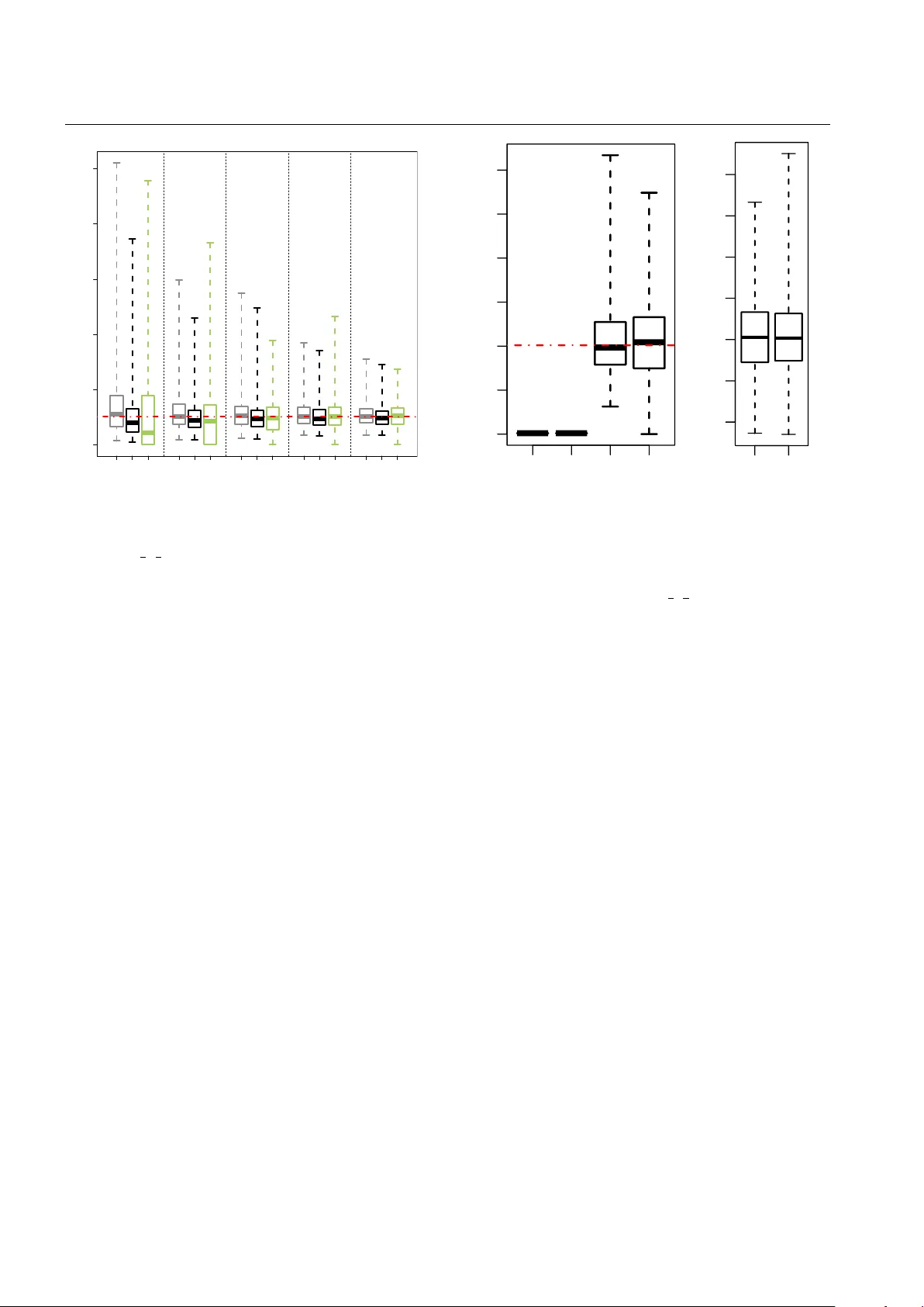
P oint Pr ocess-based Monte Carlo estimation Cl ´ ement W alter Laboratoire de Probabilit ´ es et Mod ` eles Al ´ eatoires Univ ersit ´ e Paris Diderot, P aris, France CEA, D AM, DIF , F-91297 Arpajon, France T el.: +331-69-264000 E-mail: clement.walter@cea.fr Abstract This paper addresses the issue of estimating the expectation of a real-valued random variable of the form X = g ( U ) where g is a deterministic function and U can be a random finite- or infinite-dimensional vector . Using re- cent results on rare event simulation, we propose a unified framew ork for dealing with both probability and mean es- timation for such random variables, i.e. linking algorithms such as T ootsie Pop Algorithm (TP A) or Last P article Al- gorithm with nested sampling. Especially , it extends nested sampling as follo ws: first the random v ariable X does not need to be bounded any more: it gives the principle of an ideal estimator with an infinite number of terms that is un- biased and always better than a classical Monte Carlo es- timator – in particular it has a finite variance as soon as there exists k ∈ R > 1 such that E  X k  < ∞ . Moreov er we address the issue of nested sampling termination and show that a random truncation of the sum can preserve unbiased- ness while increasing the variance only by a factor up to 2 compared to the ideal case. W e also build an unbiased es- timator with fix ed computational b udget which supports a Central Limit Theorem and discuss parallel implementation of nested sampling, which can dramatically reduce its com- putational cost. Finally we extensi vely study the case where X is heavy-tailed. Keyw ords Nested sampling · Evidence · Central limit theorem · Heavy tails · T rimmed mean · T ail index estimation · Rare e vent simulation · Last P article Algorithm 1 Introduction Nested sampling was introduced in the Bayesian framew ork by Skilling (2006) as a method for “estimating directly how the likelihood function relates to prior mass”. Formally , it builds an approximation for the e vidence: Z = Z Θ L ( θ ) π ( θ ) d θ , where π is the prior distribution, L the likelihood, and Θ ⊂ R d . It is somehow a quadrature formula but in the [ 0 , 1 ] in- terval rather than in the original multidimensional space Θ : Z = Z 1 0 Q ( P ) d P , where Q is the quantile function which is the generalised in verse of: P ( λ ) = Z L ( θ ) > λ π ( θ ) d θ . Hence the name nested sampling because the initial input space is divided into nested subsets { θ ∈ Θ | L ( θ ) > λ } . Con vergence of the approximation error toward a Gaussian distribution has been pro ved (Chopin and Robert 2010) when assuming that Q is twice continuously dif ferentiable with its two first deri v ativ es bounded ov er [ ε , 1 ] for some ε > 0. On the other hand estimating a quantity such as P ( λ ) for a gi ven λ is a typical problem arising in rare e vent prob- ability estimation. In this context, L (often denoted by g ) represents a complex computer code (not necessarily pos- itiv e valued nor continuous nor bounded), θ is a vector of parameters, and F λ = { θ ∈ Θ | L ( θ ) > λ } is the so-called failure domain. The idea of writing F λ as a finite intersection 2 of nested subsets F λ 0 ⊃ · · · ⊃ F λ n , − ∞ = λ 0 < · · · < λ n = λ goes back to Kahn and Harris (1951) and is now referred to as Multilev el Splitting (Garvels 2000; C ´ erou and Guyader 2007) or Subset Simulation (Au and Beck 2001). Statistical properties and con ver gence results have been deri ved by in- terpreting the Splitting algorithm in terms of an Interacting Particles System (C ´ erou et al 2009, 2012). Furthermore a particular implementation, sometimes called the Last P arti- cle Algorithm (LP A), has gained a lot of attention and Hu- ber et al (2011, 2014), Guyader et al (2011) and Simon- net (2014) hav e independently proved its link with a Pois- son process. This algorithm is indeed someho w the one pro- posed by Skilling (2006, Section 6) but the connection be- tween nested sampling and rare event simulation remains unclear (see Guyader et al (2011) and the discussion follo w- ing Huber et al (2011) in Bernardo et al (2011)). The goal of this paper is to fill this gap by introduc- ing a common frame work for these methodologies. The core tool is that any continuous real-v alued random variable can be linked with a Poisson process with parameter 1. Then a family of estimators can be defined using sev eral realisa- tions of such processes instead of iid samples. While it only recasts results for extreme probability estimation in a very general setting – i.e. the random variable of interest writes as X = g ( U ) ∈ R where g is a deterministic function and U can be a random finite- or infinite-dimensional vector – it extends nested sampling to the estimation of the mean of any real-valued random variables (bounded or not) and brings ne w theoretical results: 1) the ideal estimator with an infinite number of terms (non truncated nested sampling) is unbiased; 2) the ideal nested sampling estimator is always better than the classical Monte Carlo estimator in term of variance; and 3) it has a finite v ariance as soon as a moment of order k ∈ ( 1 , ∞ ) e xists. Moreov er we address the issue of the nested sampling termination (see Skilling 2006, Section 7). Using results on Multilev el Monte Carlo (Giles 2008; McLeish 2011; Rhee and Glynn 2013), we show that one can get an unbiased es- timator with a random but a.s. finite number of terms whose variance is only twice the one of the ideal estimator . W e also build an unbiased estimator with a fix ed computational bud- get which supports a Central Limit Theorem. W e further dis- cuss parallel implementation of nested sampling and these new estimators as this can can dramatically reduce its com- putational cost. All these theoretical results are derived assuming that it is possible to generate samples according to conditional laws when it is required. This is indeed a tough require- ment b ut this problem is well identified and not particular to these randomised estimators (see Roberts 2011); especially Skilling (2006); Huber et al (2011); Guyader et al (2011) al- ready acknowledge it and make use of Mark ov Chain Monte Carlo sampling. While a lot of ongoing work on nested sam- pling focus on impro ving these conditional simulations ( e.g . Brewer et al 2011), in the present article we focus on theo- retical statistical properties and suggest a possible solution to the issue of choosing a bad stopping criterion. Hence, it is out of the scope of the present work to benchmark nested sampling against other tailor-made methods such as Impor- tance Sampling (see for example (Robert and Casella 2004) or (Glynn and Iglehart 1989)) on a list of specific cases. The outline of this paper is as follows: Section 2 presents the common frame work for rare e vent simulation and nested sampling and deri ves a new ideal (not practically imple- mentable) estimator of m = E [ X ] = E [ g ( U )] . It is closely related to nested sampling with an infinite number of terms and is compared to the usual Monte Carlo estimator . Sec- tion 3 proposes two possible estimators based on the ideal one. Section 4 studies the specific case where X = g ( U ) is heavy-tailed and Section 5 giv es information on practical implementation and numerical results. Finally an Appendix gathers all the proofs. 2 Ideal estimator From now on we consider a real-valued random variable X , which can be for instance the output of a mapping X = g ( U ) , as discussed in the Introduction. Furthermore for a real-valued random variable X , one can write X = X + − X − with X + and X − non-negati ve ran- dom variables. Then, E [ X ] = E [ X + ] − E [ X − ] . Thus in the sequel and without loss of generality we assume that X is a non-negati ve random v ariable with law µ X . W e also assume that X has a continuous cdf F and we write p x instead of P [ X > x ] = 1 − F ( x ) , for any x ∈ R + . 2.1 Extreme event simulation In this section we recast common results from (Huber et al 2011; Guyader et al 2011; Simonnet 2014) in a general frame- work. Definition 1 (Increasing random walk) Let X 0 = 0 and de- fine recursiv ely the Markov sequence ( X n ) n such that ∀ n ∈ N : P [ X n + 1 ∈ A | X 0 , · · · , X n ] = µ X ( A ∩ ( X n , + ∞ )) µ X (( X n , + ∞ )) . In other words ( X n ) n is a strictly increasing sequence where each element is generated conditionally greater than the pre- vious one. Considering the sequence ( T n ) n ≥ 1 such that T n = − log ( P [ X > X n ]) , it can be shown that ( T n ) n ≥ 1 is distributed as the arriv al times of a Poisson Process with parameter 1. Thus, the counting random v ariable of the number of ev ents before x : M x = card { n ≥ 1 | X n ≤ x } follows a Poisson law with parameter t x = − log p x . 3 This result leads to the construction of a new estima- tor for the probability of exceeding a threshold x . Indeed Lehmann-Scheff ´ e theorem states that the minimum-variance unbiased estimator (MVUE) for p x = e − t x is b p x =  1 − 1 N  M (1) with M = ∑ N i = 1 M i x the sum of N iid realisations of M x . Here we find back the LP A estimator , which means that LP A is only one possible practical implementation of this estimator; especially W alter (2015) shows that LP A generates a mark ed Poisson Process with parameter N . In any case, the statistical properties of b p x are then well known: Proposition 1 (Statistical pr operties of b p x ) E [ b p x ] = p x var [ b p x ] = p 2 x  p − 1 / N x − 1  This estimator exhibits a logarithmic efficiency and asymp- totically achieves the Cramer-Rao bound − p 2 x log p x / N . Com- paring to classical Monte Carlo, it r eplaces the factor 1 / p x in the variance by log 1 / p x when p x  1 and N  1: classical Monte Carlo Poisson Process V ariance p x ( 1 − p x ) N p 2 x  p − 1 / N x − 1  Approx. p 2 x N 1 p x p 2 x N log 1 p x Remark 1 The MVUE of t x = − log p x is M / N . From this relation one could consider the suboptimal estimator for p x : e p x = e − M N =  e − 1 N  M . (2) From the moment-generating function of M we get the mean and variance of ˜ p x : E [ e p x ] = p N ( 1 − e − 1 / N ) x = p x + − p x log p x 2 N + o  1 N  var [ b p x ] = p N ( 1 − e − 2 / N ) x − p 2 N ( 1 − e − 1 / N ) x = − p 2 x log p x N + p 2 x log p x N 2 ( log p x + 1 ) + o  1 N 2  . Hence this suboptimal estimator has a positive bias of or- der 1 / N . The variances v ar [ e p x ] and v ar [ b p x ] dif fer only from order 1 / N 2 and var [ b p x ] < var [ e p x ] as soon as p x < e − 1 . 2.2 Definition of the moment estimator Noticing that for a non-neg ativ e real-valued random variable with mean m = E [ X ] = E [ g ( U )] one has: m = Z ∞ 0 p x d x , (3) the idea is to use the optimal estimator of p x (Eq. (1)) to build an estimator for m . From no w on we will assume that N ≥ 2 point processes hav e been simulated and denote by ( M x ) x the counting ran- dom variables associated with the marked Poisson Process: ∀ x > 0 , M x ∼ P ( − N log p x ) . The sequence ( X n ) n ≥ 1 is the cumulated one, i.e. the combination of the states of the N Markov Chains sorted in increasing order; then the associ- ated ( T n ) n ≥ 1 are the times of the marked Poisson Process with parameter N . W e set X 0 = 0 and then consider the fol- lowing estimator: b m = Z ∞ 0  1 − 1 N  M x d x = ∞ ∑ i = 0 ( X i + 1 − X i )  1 − 1 N  i . (4) The second equality comes from the fact that x 7→ M x is con- stant equal to i on each interval [ X i , X i + 1 ) : there are 0 ev ent before X 1 , then 1 ev ent before X 2 , precisely at X 1 , etc. While the first form is easier to analyse because the law of ( M x ) x is well determined, the second one pav es the way for the practical implementation (see Section 3) and clarifies the link with Nested Sampling: b m = ∞ ∑ i = 1 X i "  1 − 1 N  i − 1 −  1 − 1 N  i # . (5) This estimator is the limit of the nested sampling estimator with a deterministic scheme (Skilling 2006): e m = ∞ ∑ i = 1 X i  e 1 − i N − e − i N  (6) with slightly modified weights: ( 1 − 1 / N ) instead of e − 1 / N . This is a direct consequence of the fact that an optimal un- biased estimator for e − t x is not e − ˆ t x (see Section 2.1 Remark 1). Proposition 2 (Statistical properties of b m ) E [ b m ] = m (7) var [ b m ] = 2 Z ∞ 0 Z x 0 p x p 1 − 1 / N x 0 d x 0 d x − m 2 (8) W e thus have defined an unbiased estimator for m . Remark 2 As a matter of comparison, e m can also be written e m = R ∞ 0 e p x d x . Then Remark 1 allows us to conclude that ˜ m has a positiv e bias of order 1/N. 4 Proposition 3 (Finiteness of var [ b m ] ) ∀ N ≥ 2 , v ar [ b m ] ≤ 2 1 + 1 / N E [ X 1 + 1 / N ] 2 / ( 1 + 1 / N ) . Corollary 1 (V alue of N ) Let ε > 0 , if E  X 1 + ε  < ∞ then for any N ≥ 1 / ε , b m has a finite variance. While the usual Monte Carlo estimator requires the finite- ness of E  X 2  to have a finite variance, this estimator only requires the finiteness of a moment of order 1 + ε . This is especially interesting when X is heavy-tailed and this case is further in vestigated in Section 4. 2.3 Comparison with classical Monte Carlo As the finiteness condition of the variance of b m is much weaker than for a nai ve Monte Carlo estimator, one can ex- pect a globally lower v ariance. This result is sho wn in Propo- sition 4. W e first recall the crude Monte Carlo estimator: b m MC def = 1 N N ∑ i = 1 X i (9) with ( X i ) i N iid random variables with law µ X . Proposition 4 F or any N ≥ 2 , var [ b m ] ≤ var [ b m MC ] . Thus the ideal nested sampling estimator (5) is always bet- ter than classical Monte Carlo in terms of variance and es- pecially does not require the finiteness of the second-order moment of X to hav e a finite v ariance. 3 Randomised unbiased estimator The ideal estimator (4) defined in Section 2 is not directly usable as it requires to simulate an infinite number of terms in sum (4). While the usual nested sampling implementa- tions propose to stop the algorithm either after a giv en num- ber of iterations, or according to some criterion estimated at each iteration, we propose a randomised unbiased estimator using recent results on paths simulation. 3.1 Definition W e are facing the issue of estimating E [ b m ] while it is not possible to generate such a b m in a finite computer time. This problem is well identified in the field of Stochastic Differ - ential Equations (SDE) where one often intends to compute the e xpectation of a path functional while only discrete-time approximations are available. Recently there have been two major breakthroughs that address this issue: first the Multi- lev el Monte Carlo (MLMC) method (Giles 2008) has intro- duced the idea of combining intelligently dif ferent biased es- timators (lev els of approximations) to speed up the conv er- gence and reduce the bias; then McLeish (2011) and Rhee and Glynn (2013) have introduced a general approach to constructing unbiased estimator based on a family of biased ones. Basically in our context it randomises the number of simulated steps of the Markov chain, and slightly modifies the weights of the nested sampling to r emove the bias of the final estimator . More precisely let us consider the truncated estimators ( b m n ) n ≥ 1 : b m n = Z X n 0  1 − 1 N  M x d x = n − 1 ∑ i = 0 ( X i + 1 − X i )  1 − 1 N  i and T a non-negati ve integer-v alued random variable inde- pendent of ( X n ) n ∈ N such that ∀ i ∈ N , P [ T ≥ i ] def = β i > 0; one builds the follo wing estimator (with b m 0 = 0): b Z = ∞ ∑ n = 0 b m n + 1 − b m n P [ T ≥ n ] 1 T ≥ n = T ∑ n = 0 b m n + 1 − b m n P [ T ≥ n ] = ∞ ∑ n = 0 ( X n + 1 − X n )  1 − 1 N  n 1 T ≥ n P [ T ≥ n ] . (10) Remark 3 The notation b Z might seem a bit confusing since Z is used in the Introduction for the evidence as in (Skilling 2006). This is to keep consistency with Rhee and Glynn (2013) notations where the randomising procedure comes from. Proposition 5 (Statistical properties of b Z ) E h b Z i = m var h b Z i = ∞ ∑ i = 0 q i , N β − 1 i − m 2 with: q i , N = 2  1 − 1 N  2 i Z ∞ 0 Z ∞ x 0 p x p N − 1 x 0 [ − N log p x 0 ] i i ! d x d x 0 . (11) The asymptotic behaviour of the sequence ( q i , N ) i will drive the possible choices for the randomising distribution ( β i ) i : var h b Z i to remain finite implies that q i , N β − 1 i → 0 when i → ∞ . Lemma 1 The sequence ( q i , N ) i goes to 0 at least at ex- ponential rate . Furthermore, if X has density f X such that k f X k ∞ < ∞ , it is also bounded fr om below by an exponen- tially decr easing sequence. 5 Then it appears that the Geometric distribution plays a key role, as already stated by McLeish (2011). Hence we pro- vide some theoretical results assuming that T is a geometric random variable. Proposition 6 If P [ T ≥ n ] = e − β n , β > 0 , then: var h b Z i = 2 Z ∞ 0 Z x 0 p x p 1 − 1 γ ( β , N ) x 0 d x 0 d x − m 2 (12) with γ ( β , N ) = N / ( 1 + ( e β − 1 )( N − 1 ) 2 ) . This e xpression is indeed the same as the one of Proposition 2 with the function γ ( β , N ) instead of N . Hence the greater γ the smaller var h b Z i . Furthermore one has directly all the results from Section 2.2, especially the finiteness conditions for the variance giv en in Proposition 3 and Corollary 1, re- placing N by γ ( β , N ) . While there is no value of β minimising var h b Z i at a giv en N (the smaller β the smaller the variance of the ran- domised estimator b Z ), there is an optimal v alue for N at a giv en β , i.e. for a giv en finite computational budget: N = p 1 + E [ T ] . One can reverse this relation, which gi ves: β app def = log  1 + 1 / ( N 2 − 1 )  . (13) Corollary 2 Let N ≥ 2 and P [ T ≥ n ] = e − n β app ( N ) , then: var h b Z i ( N ) = v ar [ b m ] ( N + 1 2 ) ≈ 2 var [ b m ] ( N ) . (14) This means that instead of choosing an arbitrary stopping criterion for nested sampling, randomising the number of it- erations and computing b Z allows for keeping an unbiased es- timator without increasing drastically the variance (factor up to 2, reached with suboptimal implementation of Corollary 2). This result will be illustrated in the examples of Section 5. 3.2 Conv ergence rate Throughout the paper we consider that the computational cost for generating a realisation of b Z is the number of sim- ulated samples. Accordingly , in this section it is the number of calls to a simulator of a conditional law . Proposition 7 Let τ be the random variable of the number of samples r equir ed to generate b Z . One has τ = N + T . Corollary 3 (Conv ergence rate of b Z ) F or any non-negative inte ger-valued randomising variable T such that E [ T ] < ∞ and ∀ i ∈ N , P [ T ≥ i ] > 0 , one has: E [ τ ] · var h b Z i ≥ 2 q 1 , 2 + O  1 N  , N → ∞ . (15) If the inequality (15) is close to an equality then b Z has a canonical square-root con ver gence rate (as a function of the computational cost). Howe ver there is no guarantee on this rate of conv ergence. Especially Corollary 4 below shows that it is not the case when T has a geometric distribution. Corollary 4 If T is a Geometric random variable such that ∀ n ∈ N , P [ T ≥ n ] = e − β n with β = Θ ( 1 / N 1 + ε ) , ε ≥ 0 , then:    E [ τ ] · var h b Z i = Θ ( N ) ε ∈ [ 0 , 1 ] E [ τ ] · var h b Z i = Θ ( N ε ) ε > 1 . Hence the unbiased randomised estimator of Corollary 2 with β = β app = Θ ( 1 / N 2 ) does not have a canonical square- root con ver gence rate. Furthermore, e ven though the realisa- tion of the geometric random variable giv es a small number of iterations, one may want to run the algorithm longer to probe the tail of the likelihood function to make sure that no important part is missing (Skilling 2006). That is why the idea behind randomised estimators is to av erage several replicas of b Z because it will somehow av erage the quanti- ties 1 T ≥ n / P [ T ≥ n ] in (10). More precisely , let G ( c ) be the random v ariable of the number of simulations of b Z one can afford with a computational b udget c : G ( c ) = max { n ≥ 0 | n ∑ i = 1 τ i ≤ c } where τ i is the computational ef fort required to generate the i t h -sample b Z i , one considers the following estimator: b α ( c ) = 1 G ( c ) G ( c ) ∑ i = 1 b Z i . (16) In this setting Glynn and Whitt (1992) showed a CL T -like result: c 1 / 2 ( b α ( c ) − E h b Z i ) L − − − → c → ∞ ( E [ τ ] · var h b Z i ) 1 / 2 N ( 0 , 1 ) . (17) Hence in our context one has to tune ( β i ) i and N to minimise the product E [ τ ] · var h b Z i . 3.3 Optimal randomisation Since T is a non-negati ve random variable one has P [ T ≥ 0 ] = β 0 = 1. Let C = { ( β i ) i ∈ ( 0 , 1 ] N | β 0 = 1 and ∀ i ∈ N , β i + 1 ≤ β i } ; we intend to solve the optimisation problem: argmin ( β i ) i ∈ C N ∈ J 2 , ∞ ) E [ τ ] · var h b Z i = argmin ( β i ) i ∈ C N ∈ J 2 , ∞ ) N − 1 + ∞ ∑ i = 0 β i ! ∞ ∑ i = 0 q i , N β − 1 i − m 2 ! (18) 6 where the ( q i , N ) i are given by (11). Furthermore, one can rewrite the ( q i , N ) i assuming that X has a density f X > 0. Indeed in this context X n has a density f n such that: ∀ n ≥ 1 , f n ( x ) = N p N − 1 x ( − N log p x ) n − 1 ( n − 1 ) ! f X ( x ) . This giv es: ∀ i ∈ N , q i , N = 2 N  1 − 1 N  2 i E [ R ( X i + 1 )] with R ( x ) = R ∞ x p u d u / f X ( x ) . Hence we further assume that ( q i , N ) i is decreasing, which is the case for a Pareto random variable (see Section 4.1) and at least for any distribution for which R is non-increasing like e xponential and uniform distributions. In this conte xt Proposition 8 gi ves the optimal distribution for T for a giv en N . Proposition 8 (Optimal distribution f or T ) If ( q i , N ) i ≥ 1 is decr easing then the optimal distribution ( β ∗ i ) i for T is given by: ∀ i ∈ J 0 , i 0 K , β ∗ i = 1 ∀ i > i 0 , β ∗ i = r N + i 0 S 0 √ q i , N with i 0 = min { i ∈ N | ∑ i j = 0 q j , N − m 2 > ( N + i ) q ( i + 1 ) , N } and S 0 = ∑ i 0 j = 0 q j , N − m 2 . It is part of the proof in the appendix that i 0 is well defined and so it appears that the optimal distribution enforces the estimator to go at least until the i t h 0 ev ent. Recalling ( X n ) n is the cumulated Marko v Chain (associated with the marked Poisson Process with parameter N ), this can be understood in the sense that on av erage, at least N ev ents are neces- sary to use at least one time each process. Even if the link between i 0 and N is not that straightforward, one can then conjecture that lim N → ∞ i 0 = ∞ . Corollary 5 (Bounds on β ∗ i ) F or all i > i 0 , one has: r q i , N q i 0 + 1 , N > β ∗ i ≥ r q i , N q i 0 , N . (19) Thus the tail of the optimal distribution ( β ∗ i ) i is exponen- tially decreasing by Lemma 1. From these bounds on the ( β i ) i one can also deriv e bounds on the variance: q i 0 + 1 , N E [ τ ] 2 < E [ τ ] · var h b Z i ≤ q i 0 , N E [ τ ] 2 . Assuming lim N → ∞ i 0 = ∞ and using the lower bound on q i , N from Lemma 1, one can show that lim N → ∞ E [ τ ] · var h b Z i = ∞ , which implies the existence of an optimal N . Section 4.1 presents an exact resolution of this optimisation problem for a Pareto random v ariable. Finally , we have presented in this section the frame work for an optimal resolution of Problem (18) and proven ex- istence of a solution under reasonable assumptions ( ( q i , N ) i is decreasing and lim N → ∞ i 0 = ∞ ). Furthermore the com- prehensiv e resolution in the case of a Pareto distribution in Section 4.1 legitimises these assumptions. Generally speak- ing, if ( q i , N ) i ≥ 1 is not decreasing the optimisation has to be performed over all the decreasing sub-sequences of ( q i , N ) i , which turns it into a combinatorial problem (see Rhee and Glynn 2013, Theorem 3). 3.4 Geometric randomisation On the one hand the computation of the optimal distribution for T can be quite demanding in computer time; and on the other hand the geometric law plays a k ey role as for any dis- tribution p x , the sequence ( q i , N ) i decreases at exponential rate and the optimal randomising distribution (when ( q i , N ) i is decreasing) is somehow a shifted geometric law . There- fore we study the parametric case where P [ T ≥ n ] = e − β n , β > 0 and tune β and N to minimise E [ τ ] · v ar h b Z i . Using the exponential power series in var h b Z i (cf. Eq. (12)), the optimisation problem (18) becomes: min β > 0 N ∈ J 2 , ∞ )  N + 1 e β − 1  ∞ ∑ i = 0 q i , 2  2 γ ( β , N )  i − m 2 ! . (20) Proposition 9 There exists a global minimiser ( β opt , N opt ) to Pr oblem (20) . Furthermor e, ( β opt , N opt ) satisfies the r ela- tionship: β opt = log   1 + 2 N 2 opt − 1 + ( N opt − 1 ) q N 2 opt + 6 N opt + 1   . (21) Hence there is always an optimal solution to Problem (20), meaning this parametrisation is meaningful. T o summarise we have shown that by randomising the fi- nite number of iterations and slightly modifying the weights of the original nested sampling, it is possible to define an unbiased estimator for the mean of any real-valued random variable with continuous cdf , resolving the issue of choosing an appr opriate stopping criterion. With a suboptimal geo- metric randomisation as in Corollary 2, the variance is at most twice the one of the ideal case (estimator (4)). Ho wev er it is not usable with a fixed predetermined computational budget and its con ver gence rate is slo wer than the canonical square-root one. T o circumvent this limitation, the idea is to av erage se veral replicas of the randomised unbiased estima- tor (see Eq. (16)). This new estimator remains unbiased and also supports a Central Limit Theorem. 7 All these theoretical results assume that it is possible to generate conditional random v ariables when required, as for the original nested sampling algorithm (see Skilling 2006, Section 9). Efficient conditional simulation can be carried out in different ways, from perfect simulation (see for ex- ample Propp and Wilson 1996) to approximation using ran- dom walk Metropolis-Hastings. The aim of this paper is not to challenge this hypothesis in a general manner but only to provide a new insight on the risk of choosing a bad stop- ping criterion in nested sampling, and to propose an other tool to deal with this issue. Since nested sampling has been applied successfully to a great number of problems so far , these results are expected to hold in these situations. Also the examples of Section 5 are in good agreement with these theoretical results. In the ne xt section, we discuss the dif ferent stopping cri- teria usually recommended for nested sampling and parallel implementation of the estimators. 3.5 Parallel implementation Skilling (2006, Section 7) presents two possible termination rules based on criteria ev aluated on-the-fly: – stop when the greatest expected increment (current weight and biggest found likelihood v alue) is smaller than a giv en fraction of the current estimate; – stop when the number of iterations significantly e xceeds N H with H the information, estimated on-the-fly . Chopin and Robert (2010) use an other stopping criterion, close to the first one above, it is: “stop when the ne w in- crement is smaller than a giv en fraction of the current esti- mate”. An other option is to do a predetermined number of iterations (Brewer et al 2011). Unfortunately these criteria giv e no guarantee on the con vergence of the estimator to the sought value and may lead to biased estimation. A first difference between the three first criteria and the last one stands in the fact that this latter uses a known com- putational budget while the others ones will run until the criterion is satisfied; hence there is no way to estimate the (random) final number of iteration in adv ance. This differ - ence is also to be found between b Z and b α : the first one will use a random number of simulated samples (the dra w of the randomising variable) while the second one is defined with a fix ed computational b udget. Hence these two cate gories of estimators cannot be compared because the setting is not the same. An other main difference between these estimators is whether they enable parallel computation or not. The three first stopping criteria need to be ev aluated at each iteration and are based on quantities estimated with the full process with parameter N . Hence the y do not allo w for parallel com- putation. On the other hand, with a predetermined total num- ber of iterations, parallel computation on the model of (W al- ter 2015, Section 4.2) can be carried out. The randomised estimator b Z also enables this feature as the random number of iterations is drawn before the algorithm starts. Consider- ing b α , each replica can be computed in parallel, and further the computation of each replica also allows for parallel im- plementation. Hence b α allows for a double parallelisation, which is worth noticing as it may require a substantial com- putational budget to become ef fectively Gaussian. T o conclude, one stresses out the fact that among esti- mators with random computational budget, b Z is the only one allowing for parallel computation; furthermore it is also the only one unbiased and its variance is at worst twice the one of the ideal estimator (upper bound reached with suboptimal implementation of b Z as in Corollary 2). Both fixed-budget estimators enable parallel implementation; howe ver nested sampling with a predetermined number of iterations has no reason to be close to the sought value. On the other hand, b α is unbiased and supports a CL T . All these considerations are illustrated in Section 5. 4 Application to hea vy-tailed random variables In this section we give insights on the properties of the new estimator when X = g ( U ) is heavy-tailed. Mean estimation for heavy-tailed random v ariables is a well identified prob- lem often addressed by some parametric assumptions on the cdf of X ; see Beirlant et al (2012) for a comprehensive ov erview of tail index estimation, and Peng (2001); Johans- son (2003); Necir et al (2010); Hill (2013) for references on mean estimation for heavy-tailed random v ariables. In the sequel we then give explicit results for the Pareto distribution p x = P [ X > x ] = 1 ∧ x − a , a > 1. 4.1 Exact resolution for a Pareto distribution W ith an analytic form for the cdf of X , we can deriv e ex- plicit formulae for the variance (Eq. (8)) and the optimisa- tion problem (18). First we compare the v ariance of the ideal estimator b m against usual Monte Carlo and Importance Sampling esti- mators. In this latter case the importance density is chosen to be a Pareto distrib ution with parameter b > 0. Proposition 10 (V ariance comparison) F or a P areto dis- tribution, one has m = a / ( a − 1 ) and the variances write: a > 2 , var [ b m MC ] = m ( m − 1 ) 2 2 N − mN a > 2 N 2 N − 1 , var [ b m ] = m ( m − 1 ) 2 2 N − m a > 1 + b 2 , var [ b m I S ] = m 2 ( B − 1 ) 2 N ( 2 B − 1 ) 8 with B = ( a − 1 ) / b ∈ ( 1 / 2 , ∞ ) . It is clearly visible that the classical Monte Carlo esti- mator needs a second-order moment while b m only requires a > 2 N / ( 2 N − 1 ) ≈ 1 + 1 / 2 N and b m I S requires a > 1 + b / 2; it also illustrates the result of Proposition 4: var [ b m ] < var [ b m MC ] . The optimal value b = a − 1 cancels out var [ b m I S ] . It is well known that there is an optimal density q for IS that cancels out the variance of the IS estimator but it is case- specific: here a Pareto density with parameter a − 1. Remark 4 (Limit distribution of classical Monte Carlo es- timator) In the case of Pareto distribution, when a > 2 the Central Limit Theorem giv es the limit law of the estimator while for 1 < a < 2 the Generalised Central Limit Theorem (see for example Embrechts et al 1997) states that ∑ i X i is in the domain of attraction of a stable law with parameter a : N 1 − 1 / a 1 N N ∑ i = 1 X i − m ! 1 C a L − − − → N → ∞ X a with the characteristic function of X a , φ X a , writing φ X a ( t ) = exp [ −| t | a ( 1 − i ( tan ( π a / 2 )) sgn ( t ))] and C a the normalising constant C a = π 1 / a ( 2 Γ ( a ) sin π a / 2 ) − 1 / a . W e now detail the resolution of optimisation problems (18) and (20). Especially we first explicit the form of the sequence ( q i , N ) i defined in Eq. (11). Proposition 11 If X is a P ar eto random variable with pa- rameter a > 1 , then: ∀ i ∈ N , q i , N = 2 ( a − 1 )( aN − 2 )  a ( N − 1 ) 2 N ( aN − 2 )  i + 1 i = 0 ( a + 1 ) 2 ( a − 1 ) . Hence for a Pareto distribution ( q i , N ) i is decreasing. One can then look for i 0 , the solution of the problem i 0 = min { i ∈ N | ∑ i j = 0 q j , N − m 2 > ( N + i ) q ( i + 1 ) , N } . Whilst an exact solution can be expressed using the lower branch of the Lambert W function (see for example Corless et al 1996), the following proposition gives an asymptotic approximation when N → ∞ to precise the growth rate of i 0 . Proposition 12 If X is a P ar eto random variable, then: i 0 = N m 2  log N + log log N − log ( m 2 )  + o ( N ) , N → ∞ . Corollary 6 (Order of magnitude of E [ τ ] · var h b Z i ) E [ τ ] · var h b Z i ∼ N → ∞  m ( m − 1 ) 2  2 log N . Corollary 6 shows that E [ τ ] · var h b Z i → ∞ when N → ∞ so there is an optimal value for N that minimises E [ τ ] · var h b Z i ; a numerical resolution for several v alues of a from 1 to 3 was performed and the result is displayed in Figure 1a. W e also present in Figure 1b a comparison between the opti- mal variance (with the optimal distribution ( β ∗ i ) i and opti- mal N ) and the classical Monte Carlo one. There we can see that for a . 2 . 5 the new estimator (16) performs better in terms of variance; especially for a < 2 it remains finite while var [ b m MC ] = ∞ . As explained in Section 3.4 we consider no w a Geomet- ric random v ariable T with parameter β for the random trun- cation. Proposition 13 If X is a P ar eto random variable with pa- rameter a > 1 and ∀ n ∈ N , P [ T ≥ n ] = e − β n then: var h b Z i = m ( m − 1 ) 2 2 γ ( β , N ) − m and β opt = log  1 B + + 1  (22) wher e B + is the positive r oot of the quadratic polynomial P ( B ) : P ( B ) = 2 N opt − m ( N opt − 1 ) 2 B 2 − 2 mB −  m ( N opt − 1 ) 2 + 2 N 2 opt  . W ith this relation and the one of Eq. (21) one can deri ve the optimal parameters ( β opt , N opt ) . Figure 1a sho ws a numerical resolution of this problem for sev eral values of a ∈ ( 1 , 3 ] . Furthermore, if one considers the approximation of the optimisation problem (20) with relation (13) instead of (21), one has to minimise N 7→ ( N 2 + N − 1 ) m ( m − 1 ) 2 / ( N + 1 − m ) . Denoting N app this minimiser , one has: N app = max  m − 1 + p m 2 − m − 1 , 2  (23) This approximation is the red dotted-dashed line of Figure 1a. As we can see, it is in good agreement with the optimal values, both for the parameter N and for the global variance (see further Section 4.2 and Figure 1b). 4.2 Comparison of the estimators W e have seen in Sections 3.3 and 3.4 two ways of imple- menting the ideal estimator b m defined in Section 2.2 with a fixed computational budget. Then we hav e presented their exact behaviours in a case of a Pareto random variable. These two ways in volv e a truncation of the infinite sum (4) by an integer -v alued random variable T . In the first implementa- tion the distribution of T and the number N of point pro- cesses are optimised in order to minimise the estimator v ari- ance. In the second implementation, the distribution of T is enforced to be geometric and its parameter as well as N are optimised. 9 While the first implementation is optimal in terms of variance, it requires to solve a combinatorial problem, which can turn it into a poorer algorithm in terms of computational time. In this scope, the parametric algorithm constraining the randomising variable T to be geometric with parameter β is much simpler to implement. The aim of this section is to benchmark these two implementations and to challenge the optimal parameters against the fixed ones we will suggest. More precisely , while both optimisations ended up with optimal parameters depending on the distribution of X , we also consider the parametric algorithm with parameter β app giv en by (13) and N = N app , 2, 5 or 10. Figure 1b shows the relativ e increase of the standard de- viations due to the suboptimal implementations for a giv en computational budget, i.e. for a given number of generated samples. It also sho ws the standard de viation ratios between the optimal implementation, the classical Monte Carlo esti- mator (9) and b m giv en by (4). For this latter, it is assumed that its computational cost is N , i.e. that it costs 1 to sim- ulate an increasing random walk (see Definition 1) while it requires an infinite number of simulated samples. This calls for certain comments: – the parametric implementation with optimised parame- ters ( β opt , N opt ) remains competitiv e against the optimal implementation (solid black line going from ≈ 1 . 3 to ≈ 1 . 1); – the parametric implementation with parameters β app and N app is almost not distinguishable from the parametric implementation with optimal parameters β opt and N opt . This means that it is not necessary to strive to estimate the parameters ( β opt , N opt ) ; – the classical Monte Carlo estimator is better than the op- timal implementation as soon as a & 2 . 5 and better than the parametric implementation as soon as a & 2 . 3; this confirms that nested sampling is especially con venient for heavy-tailed random v ariables; – the standard deviation of b m illustrates the efficienc y of the ideal estimator compared to the classical Monte Carlo one (cf. Proposition 10), with a standard deviation at least twice as small; – generally speaking and without any knowledge on the distribution of X , N should not be set too small as the variance increases much faster when it is smaller than the optimal value; especially with β = β app finiteness condition of the variance writes a > 1 + 1 / N . Giv en these results we can consider that the parametric im- plementation is a good trade-off between minimal variance estimation and complexity , especially when no information on the distribution of X is provided. 1.0 1.5 2.0 2.5 3.0 2 5 10 20 50 200 500 a N optimal General Parametric Approximation (a) Optimal values for N in the general (cf Section 3.3) and in the parametric (cf Section 3.4) cases with the approximation of equation (23). a is the parameter of the Pareto distrib ution. 1.0 1.5 2.0 2.5 3.0 0.0 0.5 1.0 1.5 2.0 a σ / σ opt ( β app , N app ) ( β app , 10 ) ( β app , 5 ) ( β app , 2 ) Monte Carlo b m ( β opt , N opt ) (b) Ratios of the standard deviations of different estimators over the standard deviation of the optimal estimator b α of Section 3.3. The classical Monte Carlo estimator is defined in Eq. (9); b m is the ideal estimator (4); the other estimators are randomised estimators (16) with enforced geometric distribution for T with parameter β and N as follows: ( β opt , N opt ) : optimal parameters of Proposition 9; ( β app , N app ) : approximated optimal parameters of Eq. (13) and (23). a is the parameter of the Pareto distrib ution. Fig. 1: Theoretical resolution of problems (18) and (20) when P [ X > x ] = 1 ∧ x − a . 5 Example The aim of this section is to check the consistency between theoretical formulae and practical results with non-ideal con- 10 ditional sampling. It is also to demonstrate how bad stop- ping criteria can alter nested sampling and how randomised estimators can resolve this issue. W e first explain how we perform conditional simulation and gi ve pseudo-code for both b Z and b α . Then we present results on an example from (Skilling 2006, Section 18) that we slightly modify . The pre- sented results are obtained with 500 simulations and box- plots extend to the e xtreme values. 5.1 Simulating conditional distributions When no conditional sampler is available, a general idea is to use con ver gence properties of an ergodic Markov Chain to its unique in variant probability distribution. Assuming U is a d -dimensional random v ector with pdf f U , it means that we intend to generate a Markov Chain with stationary pdf ∝ 1 g ( u ) > x f U ( u ) . This implementation is rather simple when a reversible transition kernel is av ailable. In the sequel we make use of the transition kernel suggested by C ´ erou et al (2012) detailed on Algorithm 1 for Gaussian input space. Algorithm 1 Transition kernel for U L ∼ N ( 0 , I d ) (C ´ erou et al 2012; Guyader et al 2011) Require: initial state u , σ , burn-in b while b > 0 do Pick W from a standard multiv ariate Gaussian distribution U ∗ ← u + σ W √ 1 + σ 2 if g ( U ∗ ) > x then u ← U ∗ end if b ← b − 1 end while retur n u Because the goal is to reach the stationary state of the Markov Chain, sev eral transitions hav e to be done to insure independence between the starting point and the final sam- ple and adequacy with the targeted distribution. This number of transitions is referred to as a burn-in parameter b . Even- tually the last generated sample is kept. In theory , one can start from any point provided the burn-in is large enough but practically speaking it is profitable to start with a point approximately follo wing the targeted distrib ution as burn-in will then serve mainly independence purpose. Furthermore, the step size σ is initialised at σ = 0 . 3 and further updated after each use of the transition kernel – i.e. each b transitions – to get an acceptance rate close to 0 . 5. Remark 5 The burn-in parameter increases the cost of an estimator because it needs sev eral simulations for only one sample. In this context, the computational cost defined in Proposition 7 becomes τ = N + bT and is the number of calls to the generator of X (which amounts to generate U and to call g ). Since this increase is common to all algorithms considered here, we will not mention it any more. 5.2 Pseudo-code As explained above, we do not intend to solve the combi- natorial optimisation problem in the general case and so we present here a pseudo-code for the parametric case. Reader interested in the optimal resolution is referred to (Rhee and Glynn 2013). W e then present in Algorithm 2 how to com- pute b Z and in Algorithm 3 how to compute b α ( c ) . In this lat- ter case we assume that N and β are giv en, being optimised (with previous kno wledge or simulations) or not. Algorithm 2 Pseudo-code for b Z Require: N , β Generate T according to P [ T ≥ n ] = e − β n 2: Generate N random variables ( X i ) i = 1 .. N according to µ X times [ 0 ] ← 0; delta [ 0 ] ← 0 4: for i in 1:T do ind ← argmin j X j 6: times [ i ] ← X ind delta [ i − 1 ] ← ( times [ i ] − times [ i − 1 ]) · ( 1 − 1 / N ) i e − β i 8: Generate X ∗ ∼ µ X ( · | X > X ind ) X ind ← X ∗ 10: end for ind ← argmin i X i 12: times [ T + 1 ] ← X ind delta [ T ] ← ( times [ T + 1 ] − times [ T ]) · ( 1 − 1 / N ) T e − β T 14: b Z = T ∑ i = 0 delta [ i ] Remark 6 Note that in Algorithm 2, N is both the theoreti- cal parameter of the number of increasing random walks per b Z and the size of the population for conditional simulation purpose. Hence it should not be set too small according to the dimension of the problem. This is a side ef fect of this practical implementation. Alternativ ely one could generate sev eral b Z i sequentially to aggr e gate all the samples for con- ditional simulations. Hence N could be chosen only accord- ing to theoretical guidelines. Howe ver it would disable par- allel implementation. Some recent work on the parallel im- plementation of Sequential Monte Carlo may be used here (V er g ´ e et al 2013). Note also that it is not necessary to con- sider only the minimum of the N samples in Algorithm 2; howe ver in the context of Markov Chain drawing it is bet- ter to select the starting point in a relatively big population already following the tar geted distribution. Basically , Algorithm 3 is just a wrap-up of Algorithm 2 with an update of the remaining computational budget. If 11 Algorithm 3 Pseudo-code for b α ( c ) Require: c , N , β G ← 0; b α ← 0; while c > 0 do Generate T ∗ according to P [ T ≥ n ] = e − β n c = c − ( N + T ∗ ) ; G = G + 1; T [ G ] = T ∗ end while if c < 0 then  discard the last replica if it exceeds the budget G = G − 1; T = T [ 1 : G ] end if for g in 1:G do Start Algorithm 2 from step 2 with T = T [ g ] b α = b α + b Z end for b α = b α / G one intends to use Markov Chain simulation as presented in Section 5.1 then one has to take into account the burn-in b and update c in Algorithm 3 as follows: c = c − ( N + bT ∗ ) . 5.3 V ariance increase In this section, we intend to check the variance increase be- tween the ideal estimator b m of Section 2.2 and the subopti- mal randomised estimator of Corollary 2. T o do so, we use an example from Skilling (2006) where it is kno wn that 100 iterations per particle on av erage are enough. W e also com- pute (NS) the original nested sampling estimator , i.e. the es- timator of Eq. 6. (NS) and b m dif fer only in the weights used: exp − 1 / N instead of 1 − 1 / N ; thus they are computed in the same run. The aim is to estimate the evidence of a like- lihood with uniform prior ov er a d − dimensional unit cube: m = E [ g ( U )] = E [ X ] with: g ( u ) = 100 d ∏ i = 1 e − u 2 i  2 u 2 √ 2 π u + d ∏ i = 1 e − u 2 i  2 v 2 √ 2 π v , (24) U ∼ U  − [ 1 2 , 1 2 ] d  , d = 20, u = 0 . 01 and v = 0 . 1. This rep- resents a Gaussian “spike” of width 0 . 01 superposed on a Gaussian “plateau” of width 0 . 1. Figure 2 plots the log- likelihood log x against the log-tail distribution log p x . W e then run nested sampling with stopping criterion “num- ber of iterations = 100 N ” as well as b Z for sev eral values of N from 100 to 500. Figure 3 shows the boxplots of the esti- mators. On the one hand b Z has good conv ergence properties, on the other hand the bias and variance increase due to the original nested sampling weights is clearly visible. T able 1 summarises these numerical results: both b Z and b m are un- biased while (NS) has a bias of order 1 / N (cf Remark 2). The variance increase between b m and b Z is in good agree- ment with the theoretical relationship of Corollary 2, it is var h b Z i ( N ) = var [ b m ] (( N + 1 ) / 2 ) ≈ 2 var [ b m ] . Also the ra- tio v ar [ NS ] / var [ b m ] goes from 1 . 14 to 1 . 9. This variance in- 0 50 100 150 200 250 -100 0 100 200 300 N iter / N ∼ − log p log X Original Modified Fig. 2: Log-Likelihood against probability for the original example of Skilling (2006, Section 18) (Eq. (24)) and the modified version (Eq. (25)). Both lines are got from a sample run of nested sampling with N = 300 and stopping criterion 250 N iterations. crease appears to be of order 1 / N 2 , which is consistent with the variance increase between b p x and e p x (see Remark 1). Hence, the optimal choice of the nested sampling weights leads to significant variance reduction and removes the bias of the original nested sampling when it goes far enough . Un- biasedness can be maintained at the cost of at most doubling the variance of the estimator and ev en less compared to the currently used nested sampling weights. Furthermore, there is no need to choose (and justify) a stopping criterion for nested sampling any more. N 100 200 300 400 500 E [ NS ] 142 . 3 117 . 7 114 . 6 111 . 5 109 . 5 E [ b m ] 103 . 0 100 . 8 102 . 8 102 . 8 102 . 6 E h b Z i 111 . 9 97 . 4 100 . 4 103 . 7 102 . 4 var h b Z i / var [ b m ] 3 . 23 2 . 49 1 . 90 2 . 20 1 . 70 var [ NS ] / var [ b m ] 1 . 90 1 . 33 1 . 24 1 . 17 1 . 14 var h b Z i / var [ NS ] 1 . 71 1 . 87 1 . 54 1 . 87 1 . 5 T able 1: V ariance increase between the randomised unbiased nested sampling estimator b Z , the original biased nested sam- pling (NS) and the ideal unbiased estimator b m . 12 NS b Z 0 200 400 600 800 1000 b m NS b Z b m NS b Z b m NS b Z b m NS b Z b m N = 100 N = 200 N = 400 N = 400 N = 500 Fig. 3: Boxplots of ideal infinite nested sampling b m of Eq. (4) and (NS) of Eq. (5) and randomly truncated b Z (Corollary 2) for the estimation of E [ g ( U )] with g as in Eq. (24) and U ∼ U  − [ 1 2 , 1 2 ] d  , d = 20. (NS) Ideal nested sampling is got with N iter = 100 N as this is kno wn to be enough in this case. (NS) and b m are obtained from the same runs. The (red) dot-dashed line is the theoretical value of m . 5.4 Adaptive stopping criteria As we stated in the Introduction, one of the main concern of this paper was to point out the potential risk of using nested sampling with a bad stopping criterion. In this context we run nested sampling on the pre vious e xample with the adap- tiv e stopping criteria mentioned in Section 3.5. The first one is directly picked out from (Chopin and Robert 2010), it is “stop when the current increment is less than 10 − 8 times the current estimate”. The second one is based on the estima- tion of the information H and is the one described in the Appendix of (Skilling 2006); it is “stop when the number of iterations is greater than 2 N H ”. Figure 3 shows that for N = 500 the estimators should be well con verged and so we set N = 500. Figure 4 shows that nested sampling estimator can be not consistent if the termination rule is not well-chosen. Here both implementations miss the spike. In this context, the random truncation of b Z appears as a conservati ve practice. Howe ver , even though b Z allows for parallel computing (cf. W alter 2015, Section 4.2), b Z as well as the adaptiv e stop- ping criteria do not let w ork with a fixed computational bud- get. Y et one may have to work with fixed computational re- sources. NS-inc b m b Z 0 50 100 150 200 250 300 NS-H (a) Nested sampling estimators with adaptiv e stopping criteria, b m and b Z NS-inc 0.6 0.8 1.0 1.2 1.4 1.6 1.8 NS-H (b) Zoom on the nested sampling estimators with adaptiv e stopping criteria Fig. 4: Effect of the choice of a stopping criterion for nested sampling estimator when estimating E [ g ( U )] with g as in Eq. (24) and U ∼ U  − [ 1 2 , 1 2 ] d  , d = 20. (NS-inc): nested sampling stopped when current increment is less than 10 − 8 times the current estimator; (NS-H): nested sampling stopped when the number of iterations e xceeds 2 N H ; b m and b Z as in Figure 3. The (red) dot-dashed line is the theoretical value of m . 5.5 Nested sampling with fixed computational budget There is only one nested sampling implementation which allows for fixing the total computational budget in advance. It is the one which stops after a given number of iterations. Follo wing Rhee and Glynn (2013) we hav e proposed in Sec- tions 3.3 and 3.4 a randomised estimator which also works with a predetermined computational budget. It is still unbi- ased and supports a Central Limit Theorem. The goal of this section is to compare these two estimators. W e slightly mod- ify the pre vious e xample (24) to narro w the spik e: u = 0 . 001 instead of u = 0 . 01, and to make the random variable heavy- tailed: g ht ( u ) = g ( u ) / d ∑ i = 1 u 2 i ! 0 . 4 d . (25) Figure 2 compares this modified example with the origi- nal one. The heavy-tailed behaviour with tail inde x 1 / 0 . 8 = 1 . 25 is clearly visible (limit slope of log-likelihood is 0 . 8) as well as the effect of the narrower spike (shift of the mass from − log p ≈ 50 to − log p ≈ 90). W ith In v- χ 2 approxima- tion of 1 / ∑ U 2 i , the sought v alue is E [ g ht ( U )] ≈ 1 . 08 × 10 42 . 13 Nested sampling is run with N = 1000 and N = 10000. W e stop it after 100 N iterations as in (Brewer et al 2011). This makes a total computational budget c = 10 5 (resp. 10 6 ). b α is implemented with a suboptimal geometric randomis- ing variable with parameter β app (Eq. (13)) and N = 20. According to Remark 6, N = d because it is both the the- oretical parameter of b α and the population size for con- ditional sampling. Considering the heavy-tail behaviour of X = g ( U ) , the estimator has a finite variance as soon as a > 1 + 1 / N = 1 . 05. One the one hand we know here that the tail-index of X is equal to 1 / 0 . 8 = 1 . 25; on the other hand it is easy to check this condition afterwards by estimating the slope on the plot log X against N iter / N as in Figure 2. NS(10 5 ) NS(10 6 ) b α ( 10 5 ) b α ( 10 6 ) 1e+07 1e+15 1e+23 1e+31 1e+39 Fig. 5: Estimation of E [ g ht ( U )] with U ∼ U  − [ 1 2 , 1 2 ] d  , d = 20. (NS): nested sampling stopped after 100 N iterations; b α : estimator of Section 3.4 with β app (Eq. (13)) and N = 20. 10 5 and 10 6 are the computational budgets used. The (red) dot-dashed line is the theoretical value of m . It is visible on Figure 5 that nested sampling did not go far enough and misses an important part of the mass: E  NS ( 10 5 )  = 5 . 32 × 10 29 and E  NS ( 10 6 )  = 2 . 41 × 10 29 while the reference value is 1 . 08 × 10 42 . On the other hand, b α is unbiased (estimated means are 6 . 43 × 10 41 and 1 . 52 × 10 42 ). Ho wever , it does not seem to be approximately Gaus- sian yet. Indeed b Z can be relativ ely heavy-tailed (McLeish 2011) and a consequent computational budget may be re- quired for b α to effecti vely become normally distrib uted. 6 Conclusion Nested Sampling has been proposed as a method for esti- mating the e vidence in a Bayesian framew ork and applied with success in a great v ariety of areas like astronomy and cosmology . Since its introduction, a lot of work has been done to clarify its con ver gence properties ( e .g. Evans 2007; Chopin and Robert 2010; Keeton 2011) and to handle the issue of conditional sampling ( e.g . Mukherjee et al 2006; Brewer et al 2011; Martiniani et al 2014). Howe ver nested sampling termination remains an open issue and a matter of user judgement (Skilling 2006, Section 7). Linking nested sampling with recent results in rare e vent simulation, this paper extends it to the estimation of the mean of any real-valued random variable (being bounded or not) and goes on step further by gi ving the optimal nested sampling weights and proving that 1) an idealised nested sampling with slightly modified weights and an infinite num- ber of iterations is unbiased; 2) its variance is always lower than the classical Monte Carlo estimator one’ s; and 3) the random variable of interest does not need to hav e a finite second-order moment to produce an estimator with finite variance. This latter property makes nested sampling espe- cially relev ant for heavy-tailed random variables as devel- oped Section 4. Furthermore, we also present two ways of implement- ing a practical unbiased estimator with an a.s. finite num- ber of terms, resolving the issue of choosing an arbitrary stopping criterion. The first estimator can be used exactly as usual nested sampling and preserves unbiasedness while only doubling the variance of the ideal estimator (infinite number of terms). The second one can be used with a prede- termined fixed computational budget and supports a Central Limit Theorem. Practically speaking, they both enable par- allel implementation (unlike usual adapti ve nested sampling strategies) and do not depend on the random variable of in- terest. As for any nested sampling implementations, they re- quire to be able to generate samples according to conditional laws and theoretical results are deri ved with this hypothesis. In some cases, exact conditional sampling may be possible. When the random variable of interest is the output of a com- puter code, Markov Chain drawing like Metropolis-Hastings algorithm can overcome this issue. If only iid samples are av ailable, further work has to be done to e xplicit the link be- tween the increasing random walk presented in Section 2.1 and, for example, P areto-type distributions. Acknowledgements The author would like to thank his advisors Jos- selin Garnier (University P aris Diderot) and Gilles Defaux (Commis- sariat ` a l’Energie Atomique et aux Energies Alternati ves) for their ad- vices and suggestions as well as the revie wers for their very relev ant comments which helped improving the manuscript. This work was par - tially supported by ANR project Chorus. Appendix Proof of Pr oposition 2 one has: E [ b m ] = Z ∞ 0 E "  1 − 1 N  M x # d x = Z ∞ 0 p x d x . 14 For the variance, one uses the fact that, for x > x 0 , M x − M x 0 and M x 0 are independent to expand E  b m 2  : E  b m 2  = 2 Z ∞ 0 Z x 0 E "  1 − 1 N  M x + M x 0 # d x 0 d x = Z ∞ 0 Z x 0 E "  1 − 1 N  M x − M x 0  1 − 1 N  2 M x 0 # d x 0 d x . Furthermore renewal property of a Poisson process giv es M x − M x 0 ∼ P ( − log ( p x / p x 0 )) . Eventually one can conclude using the results of Proposition 1. u t Proof of Pr oposition 3 Starting from the expression of the variance found in Proposition 2: var [ b m ] = 2 Z ∞ 0 p x Z x 0 p 1 − 1 / N x 0 d x 0 d x − E [ X ] 2 , we make use of H ¨ older’ s inequality: Z x 0 p 1 − 1 / N x 0 d x 0 ≤  Z x 0 d x 0  1 / N  Z x 0 p x 0 d x 0  1 − 1 / N ≤ x 1 / N  Z ∞ 0 p x 0 d x 0  1 − 1 / N ≤ x 1 / N E [ X ] 1 − 1 / N . And therefore: var [ b m ] ≤ 2 1 + 1 / N E [ X ] 1 − 1 / N E h X 1 + 1 / N i . Using H ¨ older’ s inequality again, one gets: var [ b m ] ≤ 2 1 + 1 / N E h X 1 + 1 / N i 2 1 + 1 / N . u t Proof of Pr oposition 4 On the one hand one has: N v ar [ b m MC ] + m 2 = 2 Z ∞ 0 x p x d x , and on the other hand one can write: N v ar [ b m ] + m 2 = 2 Z ∞ 0 p x Z x 0 p x 0 h N ( p − 1 / N x 0 − 1 ) + 1 i d x 0 d x . Considering f : p 7→ p  N ( p − 1 / N − 1 ) + 1  , we ha ve f ( 1 ) = 1 and: f 0 ( p ) = ( N − 1 )( p − 1 / N − 1 ) ≥ 0 , ∀ p ∈ [ 0 , 1 ] . Thus: ∀ p ∈ [ 0 , 1 ] , f ( p ) ≤ 1. Therefore N v ar [ b m ] + m 2 ≤ 2 Z ∞ 0 x p x d x which shows that v ar [ b m ] ≤ var [ b m MC ] . u t Proof of Pr oposition 5 Starting with the last formulation in (10) for b Z , one uses the fact that T and ( X i ) i are independent. Finally , (4) and Proposition 2 let conclude: E h b Z i = m . For the second-order moment, we use the fact that b Z , like b m , can be written with an integral: b Z = Z ∞ 0  1 − 1 N  M x 1 T ≥ M x P [ T ≥ M x ] d x and apply the same reasoning as for E  b m 2  : giv en x > x 0 , the random variables M x − M x 0 , M x 0 and T are independent, which brings: E "  1 − 1 N  M x + M x 0 1 T ≥ M x P [ T ≥ M x ] 1 T ≥ M x 0 P [ T ≥ M x 0 ] # = E "  1 − 1 N  M x − M x 0  1 − 1 N  2 M x 0 β − 1 M x 0 1 T ≥ M x P [ T ≥ M x ] # = E "  1 − 1 N  M x − M x 0  1 − 1 N  2 M x 0 β − 1 M x 0 # = p x p x 0 ∞ ∑ i = 0 e N log p x 0  − N log p x 0 ( 1 − 1 / N ) 2  i i ! β − 1 i = ∞ ∑ i = 0 p x p N − 1 x 0  − N log p x 0 ( 1 − 1 / N ) 2  i i ! β − 1 i . Then using this equality in E h b Z 2 i giv es the solution. u t Proof of Lemma 1 Let ε > 0 be such that E  X 1 + ε  < ∞ , N ∈ N | N > 1 / ε and i ≥ 0. W e further extend the defini- tion of v ar [ b m ] gi ven in Proposition 1, Eq. (8) for any N ∈ R . Proof of Proposition 3 is based on H ˆ older’ s inequality and still holds in this case, and so for Corollary 1. Hence, according to Corollary 1: ∃ N 0 ∈ R such that N 0 < N and var [ b m ] ( N 0 ) < ∞ . Furthermore, given x and x 0 one can write: p x p N − 1 x 0 ( − log p x 0 ) i = p x p 1 − 1 / N 0 x 0 p N + 1 / N 0 − 2 x 0 ( − log p x 0 ) i . Moreov er the function p : ( 0 , 1 ) 7→ p N + 1 / N 0 − 2 ( − log p ) i is bounded abov e by e − i i i ( N + 1 / N 0 − 2 ) − i . Using the Stirling lower bound i ≥ i i e − i √ 2 π i we can write: p x p N − 1 x 0 ( − log p x 0 ) i ≤ p x p 1 − 1 / N 0 x 0 i ! √ 2 π i ( N + 1 / N 0 − 2 ) i . Finally , this inequality brings: q i , N ≤ var [ b m ] ( N 0 )  N ( 1 − 1 / N ) 2 N + 1 / N 0 − 2  i 1 √ 2 π i and ( N + 1 / N − 2 ) / ( N + 1 / N 0 − 2 ) < 1, which concludes the first part of the proof. 15 Let us now assume that X has a density f X . One has: q i , N = 2 Z ∞ 0 Z x 0 p x p N − 1 x 0  − N log p x 0 ( 1 − 1 / N ) 2  i i ! d x 0 d x . Denote x L the left end point of X (remember that X is non- negati ve valued so x L ≥ 0). Then: q i , N ≥ 2 Z ∞ x L Z x x L p x p N − 1 x 0  − N log p x 0 ( 1 − 1 / N ) 2  i i ! d x 0 d x . W e then consider the change of variable u = − log p x and u 0 = − log p x 0 ; for all i ≥ 1 one has: q i , N ≥ 2 k f X k 2 ∞  1 − 1 N  2 i Z ∞ 0 e − 2 u Z u 0 e − N u 0 ( N u 0 ) i i ! d u 0 d u ≥ 2 k f X k 2 ∞  1 − 1 N  2 i Z ∞ 0 e − 2 u 1 N ∞ ∑ k = i + 1 e − N u ( N u ) k k ! d u ≥ 2 k f X k 2 ∞ 1 N ( N + 2 )  1 − 1 N  2 i ∞ ∑ k = i + 1  N N + 2  k q i , N ≥ 1 ( N + 2 ) k f X k 2 ∞ " N N + 2  1 − 1 N  2 # i . u t Proof of Pr oposition 6 Let α > 0 be such that ( 1 − 1 / N ) = e − α . The ar gument is the same one as in Proposition 5. One has: E h b Z 2 i = 2 Z ∞ 0 Z x 0 E h e − α ( M x − M x 0 ) e ( β − 2 α ) M 0 x i d x 0 d x = 2 Z ∞ 0 Z x 0 p x p 1 − 1 γ ( β , N ) x 0 d x 0 d x with: N γ ( β , N ) = 2 N − N 2 + e β ( N − 1 ) 2 = 1 + ( N − 1 ) 2 ( e β − 1 ) . u t Proof of Cor ollary 2 Noticing that for any N ≥ 2, one has γ ( β app ( N ) , N ) = ( N + 1 ) / 2 gi ves the first equality . Then, since var [ b m ] typically scales with 1 / N (usual results on nested sampling) giv es the approximation. Proof of Pr oposition 7 If T = 0 then no other simulation is done other than the first element of each Markov chain, i.e. N simulations are done. Then each step requires the simula- tion of the next stopping time, i.e. one simulation. Finally , this brings τ = N + T . Proof of Cor ollary 3 Note that v ar [ b m ] = ∞ ∑ i = 0 q i , N − m 2 . Hence, one has var h b Z i > v ar [ b m ] because var h b Z i = v ar [ b m ] ⇔ ∀ i ∈ N , β i = P [ T ≥ i ] = 1 and E [ τ ] > N because E [ τ ] = N ⇔ E [ T ] = 0 while ∀ i ∈ N , P [ T ≥ i ] > 0. Furthermore, the power series expansion of the exponential function and the domi- nated con vergence theorem let us re write v ar [ b m ] : var [ b m ] = ∞ ∑ i = 1 2 Z ∞ 0 Z ∞ x 0 p x p x 0 ( − log p x 0 ) i N i i ! d x d x 0 var [ b m ] = ∞ ∑ i = 1 q i , 2  2 N  i which brings: var [ b m ] = q 1 , 2 · 2 / N + O  1 / N 2  . All together, these inequalities complete the proof. u t Proof of Cor ollary 4 Denote B = 1 / ( e β − 1 ) ; one has: N + B γ ( B , N ) = N + B N + N 2 B − 1 − 2 N B + 1 B + 1 N . W ith β = Θ ( 1 / N 1 + ε ) , ε ≥ 0, one has B ∼ 1 / β ∼ N 1 + ε . Fi- nally , this giv es: N + B γ ( B , N ) ∼ N + N ε + N 1 − ε + O ( 1 ) , which concludes the proof. u t Proof of Pr oposition 8 First one shows that i 0 is well deter- mined. The sequence ( ∆ i ) i defined by: ∀ i ∈ N , ∆ i = i ∑ j = 0 q j , N − m 2 − ( N + i ) q ( i + 1 ) , N is increasing: ∆ i + 1 − ∆ i = q ( i + 1 ) , N − ( N + i + 1 ) q ( i + 2 ) , N + ( N + i ) q ( i + 1 ) , N = ( N + i + 1 )( q ( i + 1 ) , N − q ( i + 2 ) , N ) > 0 . Furthermore q 0 − m 2 = 2 Z ∞ 0 Z ∞ x 0 p x p x 0  p N − 2 x 0 − 1  d x d x 0 ≤ 0 < N q 1 , N , so ∆ 0 < 0, and ∆ i → v ar [ b m ] when i → ∞ because ( q i , N ) i decreases at exponential rate. So there exists i 0 ∈ N | ∆ i 0 − 1 ≤ 0 and ∆ i 0 > 0. Let us now consider the auxiliary problem: argmin ( β i ) i ≥ 1 β i > 0 β + ∞ ∑ i = 1 β i ! q + ∞ ∑ i = 1 q i , N β − 1 i ! with β > 0 and q ∈ R . W e show that it has a solution if and only if q > 0. Let i ≥ 1, cancelling the partial deriv atives brings: ∀ i ≥ 1 , 0 = q + ∞ ∑ j = 1 q j β − 1 j ! + β + ∞ ∑ j = 1 β j ! − q i , N β 2 i . 16 Then the solution should be of the form: ∀ i ∈ J 1 , ∞ ) , β i = c 0 √ q i for some c 0 > 0. Solving now the problem with c 0 , the deriv ative writes q − β / c 2 0 . If q ≤ 0 then it is strictly decreasing and there is no global minimiser . On the contrary , q > 0 brings c 0 = p β / q and ∀ i ≥ 1 , β i = c 0 √ q i . Thus, in our context with the constraint ∀ i ∈ N , β i ≤ 1, this means that solving the optimisation problem will set iterativ ely β i = 1 until the minimiser is feasible, i.e. until i 0 def = min { i ∈ N | i ∑ j = 0 q j , N − m 2 > ( N + i ) q ( i + 1 ) , N } . Then the solution will be giv en by: ∀ i ∈ J 1 , i 0 K , β i = 1 ∀ i > i 0 , β i = √ q i , N s 1 N + i 0 i 0 ∑ j = 0 ( q j , N − m 2 ) . u t Proof of Cor ollary 5 By definition of i 0 , one has: ( N + i 0 ) q i 0 + 1 < i 0 ∑ j = 0 q j − m 2 ≤ ( N + i 0 − 1 ) q i 0 + q i 0 which concludes the proof. u t Proof of Pr oposition 9 Denote: Q N ( β ) =  N + 1 e β − 1  ∞ ∑ i = 0 q i , 2 ( 2 / γ ) i − m 2 ! the quantity one seeks to minimise. First, we show that for any fix ed N , there exists a global minimiser of Q N ( β ) . One has Q N ( β ) → ∞ when β → 0 and γ ( β , N ) → 0 when β → ∞ . Hence, either ∃ β ∞ ∈ ( 0 , ∞ ] such that:    Q N ( β ) − − − − → β % β ∞ ∞ Q N ( β ) < ∞ ∀ β < β ∞ . Then Q N is continuous on ( 0 , β ∞ ) with infinite limits on 0 and β ∞ , so it reaches its minimum on ( 0 , β ∞ ) ; or ∃ β ∞ ∈ ( 0 , ∞ ) such that: ( Q N ( β ) < ∞ ∀ β ∈ ( 0 , β ∞ ] Q N ( β ) = ∞ ∀ β > β ∞ . Since Q N is continuous on β − ∞ by Monotone Conv ergence Theorem, Q N reaches its minimum on ( 0 , β ∞ ] . Let β opt ( N ) > 0 be such that inf β Q N ( β ) = Q N ( β opt ) . W e now show that there exists an optimal N . It is sufficient to show Q N ( β opt ) → ∞ when N → ∞ . Denote B = 1 / ( e β − 1 ) ; one has: 1 γ ( B , N ) = 1 N + N B − 2 B + 1 N B . Hence, depending on the gro wth rate of B when N → ∞ , one would ha ve: B = O ( N ) , 1 γ ∼ N B ⇒ inf β Q N ( β ) − − − → N → ∞ ∞ N = o ( B ) , 1 γ ∼ 1 N or N B ⇒ inf β Q N ( β ) ∼ B N or N ⇒ inf β Q N ( β ) − − − → N → ∞ ∞ . Then in any cases Q N ( β opt ) → ∞ when N → ∞ , which means that there exists N opt ∈ N | Q N opt ( β opt ) = inf N Q N ( β opt ) . W e now show the relationship between β opt and N opt : the partial deriv atives of E [ τ ] · var h b Z i against B and N write:            ∂  E [ τ ] · var h b Z i ∂ B = var h b Z i + E [ τ ] ∂ var h b Z i ∂ γ ∂ γ ∂ B ∂  E [ τ ] · var h b Z i ∂ N = var h b Z i + E [ τ ] ∂ var h b Z i ∂ γ ∂ γ ∂ N . At point ( β opt , N opt ) , both equations are cancelled, which giv es: ∂ γ ∂ N ( B opt , N opt ) = ∂ γ ∂ B ( B opt , N opt ) . Recalling γ ( B , N ) = N B / ( B + ( N − 1 ) 2 ) , this giv es the equa- tion: B 2 opt − ( N 2 opt − 1 ) B opt − N opt ( N opt − 1 ) 2 = 0. One can solve it in B opt and keep the positiv e root, which giv es the solution. Proof of Pr oposition 10 For the first equality: E [ X ] = Z ∞ 0 p x d x = a a − 1 var [ b m MC ] = 1 N  E  X 2  − E [ X ] 2  = a N ( a − 2 )( a − 1 ) 2 = m ( m − 1 ) 2 ( 2 − m ) N ; for the second one: E  b m 2  = 2 Z ∞ 0 Z x 0 p x p 1 − 1 / N x 0 d x 0 d x = 2 Z 1 0 Z x 0 · · · + 2 Z ∞ 1 Z 1 0 · · · + 2 Z ∞ 1 Z x 1 · · · = 1 + 2 a − 1 + 2 ( a − 1 )( 2 ( a − 1 ) − a / N ) var [ b m ] = a N ( a − 1 ) 2 ( 2 ( a − 1 ) − a / N ) ; and for the third one: var [ b m I S ] = 1 N  Z ∞ 1 x 2 a 2 b x − 2 a + b − 1 d x − a 2 ( a − 1 ) 2  var [ b m I S ] = a 2 N ( a − 1 ) 2  1 B ( 2 − B ) − 1  with B = b / ( a − 1 ) . u t 17 Proof of Pr oposition 11 Let i ≥ 0, one has: Z ∞ 1 Z ∞ x 0 p x p N − 1 x 0  − N log p x 0 ( 1 − 1 / N ) 2  i i ! d x d x 0 =  aN ( 1 − 1 / N ) 2  i i ! Z ∞ 1 Z ∞ x 0 x − a x 0− a ( N − 1 ) ( log x 0 ) i d x d x 0 =  aN ( 1 − 1 / N ) 2  i ( a − 1 ) i ! Z ∞ 1 x 0 1 − aN ( log x 0 ) i d x 0 =  aN ( 1 − 1 / N ) 2  i ( a − 1 ) i ! Γ ( i + 1 ) ( aN − 2 ) i + 1 = 1 ( a − 1 )( aN − 2 ) " aN aN − 2  1 − 1 N  2 # i with Γ standing here for the Gamma function. Furthermore: Z 1 0 Z ∞ x 0 p x p N − 1 x 0  − N log p x 0 ( 1 − 1 / N ) 2  i i ! d x d x 0 = 1 i = 0 ( a + 1 ) 2 ( a − 1 ) . ( q i , N ) i is decreasing iff: aN aN − 2  1 − 1 N  2 < 1 ⇔ 1 < a  1 − 1 2 N  which is indeed the condition for the finiteness of var [ b m ] already stated in Proposition 10. u t Proof of Pr oposition 12 The problem can be re written: min  i ≥ 1 | 1 1 − β − aN − 2 2 ( a − 1 ) > β i + 1  N + i + 1 1 − β  . Furthermore one has: 1 1 − β = N m 2 + ( a − 2 ) 2 4 ( a − 1 ) 2 + o ( 1 ) which brings that the left hand term is equal to ( m / 2 ) 2 + o ( 1 ) . Writing i = N ( k 0 + k 1 log N + k 2 log log N ) brings: β i + 1 = e − 2 k 0 m N − 2 k 1 m ( log N ) − 2 k 2 m ( 1 + o ( 1 )) . Hence one has to choose k 0 , k 1 and k 2 such that the right hand term also equals ( m / 2 ) 2 + o ( 1 ) , which giv es the solu- tion. u t Proof of Cor ollary 6 Using the asymptotic expansion of i 0 one finds q i 0 ∼ ( N 2 log N ) − 1 ( m − 1 ) 2 . Furthermore, one has E [ τ ] ∼ i 0 . Finally , the use of E [ τ ] · var h b Z i ∼ q i 0 E [ τ ] 2 giv es the result. u t Proof of Pr oposition 13 One gets the expression of the v ari- ance directly from Section 2.2 with γ ( N , β ) instead of N . Then, denoting B = 1 / ( e β − 1 ) , one solves the problem: ∂ ∂ B  ( N + B )  a 2 ( a − 1 ) γ − a  = 0 . u t References Au SK, Beck JL (2001) Estimation of small failure probabilities in high dimensions by subset simulation. Probabilistic Engineering Mechanics 16(4):263–277 Beirlant J, Caeiro F , Gomes MI (2012) An overvie w and open research topics in statistics of univ ariate extremes. REVST A T -Statistical Journal 10(1):1–31 Bernardo JM, Bayarri M, Berger JO, Dawid AP , Heckerman D (2011) Bayesian Statistics 9. Oxford Univ ersity Press Brewer BJ, P ´ artay LB, Cs ´ anyi G (2011) Diffusi ve nested sampling. Statistics and Computing 21(4):649–656 C ´ erou F , Guyader A (2007) Adapti ve multile vel splitting for rare ev ent analysis. Stochastic Analysis and Applications 25(2):417–443 C ´ erou F , Del Moral P , Furon T , Guyader A, et al (2009) Rare event simulation for a static distribution. Proceedings of RESIM 2008 URL http://www .irisa.fr/aspi/fcerou/Resim Cerou et al.pdf C ´ erou F , Del Moral P , Furon T , Guyader A (2012) Sequential Monte Carlo for rare event estimation. Statistics and Computing 22(3):795–808 Chopin N, Robert CP (2010) Properties of nested sampling. Biometrika p asq021 Corless RM, Gonnet GH, Hare DE, Jeffre y DJ, Knuth DE (1996) On the lambertw function. Advances in Computational mathematics 5(1):329–359 Embrechts P , Kl ¨ uppelberg C, Mikosch T (1997) Modelling extremal ev ents: for insurance and finance, vol 33. Springer Evans M (2007) Discussion of nested sampling for bayesian computa- tions by john skilling. Bayesian Statistics 8:491–524 Garvels MJJ (2000) The splitting method in rare e vent simulation. Uni- versiteit T wente Giles MB (2008) Multilevel monte carlo path simulation. Operations Research 56(3):607–617 Glynn PW , Iglehart DL (1989) Importance sampling for stochastic sim- ulations. Management Science 35(11):1367–1392 Glynn PW , Whitt W (1992) The asymptotic efficiency of simulation estimators. Operations Research 40(3):505–520 Guyader A, Hengartner N, Matzner-Løber E (2011) Simulation and estimation of extreme quantiles and extreme probabilities. Applied Mathematics & Optimization 64(2):171–196 Hill JB (2013) Rob ust estimation for av erage treat- ment ef fects. A vailable at SSRN 2260573 URL http://dx.doi.org/10.2139/ssrn.2260573 Huber M, Schott S, et al (2011) Using tpa for bayesian inference. Bayesian Statistics 9 9:257 Huber M, Schott S, et al (2014) Random construction of interpolating sets for high-dimensional integration. Journal of Applied Proba- bility 51(1):92–105 Johansson J (2003) Estimating the mean of heavy-tailed distributions. Extremes 6(2):91–109 Kahn H, Harris TE (1951) Estimation of particle transmission by ran- dom sampling. National Bureau of Standards applied mathematics series 12:27–30 Keeton CR (2011) On statistical uncertainty in nested sampling. Monthly Notices of the Royal Astronomical Society 414(2):1418– 1426 Martiniani S, Stev enson JD, W ales DJ, Frenk el D (2014) Superposition enhanced nested sampling. Physical Re view X 4(3):031,034 McLeish D (2011) A general method for debiasing a monte carlo esti- mator . Monte Carlo Methods and Applications Mukherjee P , Parkinson D, Liddle AR (2006) A nested sampling algo- rithm for cosmological model selection. The Astrophysical Jour- nal Letters 638(2):L51 Necir A, Rassoul A, Zitikis R (2010) Estimating t he conditional tail ex- pectation in the case of heavy-tailed losses. Journal of Probability and Statistics 2010, URL http://dx.doi.org/10.1155/2010/596839 18 Peng L (2001) Estimating the mean of a heavy tailed distribution. Statistics & Probability Letters 52(3):255–264 Propp JG, Wilson DB (1996) Exact sampling with coupled markov chains and applications to statistical mechanics. Random struc- tures and Algorithms 9(1-2):223–252 Rhee Ch, Glynn PW (2013) Unbiased estimation with square root con ver gence for sde models. Submitted for publication URL http://rhee.gatech.edu/papers/RheeGlynn13a.pdf Robert CP , Casella G (2004) Monte Carlo statistical methods. Springer Roberts G (2011) Comments on ”Using TP A for Bayesian inference” by Huber , M. and Schott, S. In: Bernardo JM, Bayarri MJ, Berger JO, Dawid AP , Heckerman D, M SAF , W est M (eds) Bayesian Statistics 9, Oxford Univ ersity Press, pp 257–282 Simonnet E (2014) Combinatorial analysis of the adaptive last particle method. Statistics and Computing pp 1–20 Skilling J (2006) Nested sampling for general bayesian computation. Bayesian Analysis 1(4):833–859 V erg ´ e C, Dubarry C, Del Moral P , Moulines E (2013) On parallel im- plementation of sequential monte carlo methods: the island parti- cle model. Statistics and Computing pp 1–18 W alter C (2015) Moving particles: A parallel optimal multilev el split- ting method with application in quantiles estimation and meta- model based algorithms. Structural Safety 55(0):10 – 25