Deep Fried Convnets

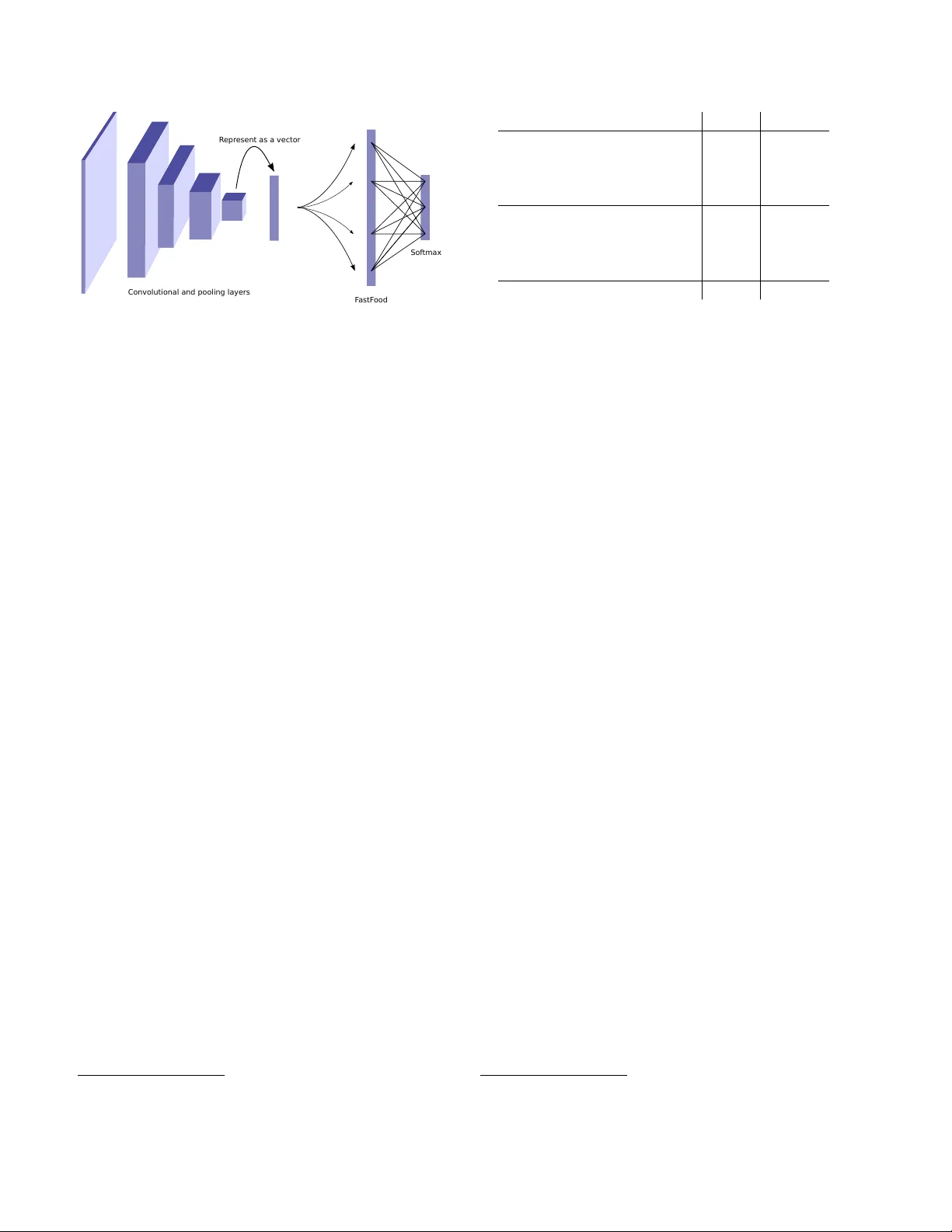
Deep Fried Con vnets Zichao Y ang 1 Marcin Moczulski 2 Misha Denil 2 , 5 Nando de Freitas 2 , 5 , 6 Alex Smola 1 , 4 Le Song 3 Ziyu W ang 2 , 5 1 Carnegie Mellon Uni versity , 2 Uni versity of Oxford, 3 Georgia Institute of T echnology 4 Google, 5 Google DeepMind, 6 Canadian Institute for Adv anced Research zichaoy@cs.cmu.edu, marcin.moczulski@stcatz.ox.ac.uk, mdenil@google.com, nandodefreitas@google.com, alex@smola.org, lsong@cc.gatech.edu, ziyu@google.com Abstract The fully- connected layers of deep con volutional neural networks typically contain over 90% of the network param- eters. Reducing the number of parameters while pr eserving pr edictive performance is critically important for training big models in distrib uted systems and for deployment in em- bedded devices. In this paper , we intr oduce a novel Adaptive F astfood transform to repar ameterize the matrix-vector multiplica- tion of fully connected layers. Reparameterizing a fully connected layer with d inputs and n outputs with the Adap- tive F astfood transform r educes the storage and computa- tional costs costs fr om O ( nd ) to O ( n ) and O ( n log d ) re- spectively . Using the Adaptive F astfood tr ansform in con vo- lutional networks r esults in what we call a deep fried con- vnet. These con vnets ar e end-to-end trainable, and enable us to attain substantial r eductions in the number of param- eters without affecting prediction accuracy on the MNIST and ImageNet datasets. 1. Introduction In recent years we hav e witnessed an explosion of ap- plications of con volutional neural networks with millions and billions of parameters. Reducing this vast number of parameters would improve the efficienc y of training in dis- tributed architectures. It would also allo w for the deploy- ment of state-of-the-art con volutional neural networks on embedded mobile applications. These train and test time considerations are both of great importance. A standard con volutional network is composed of two types of layers, each with very dif ferent properties. Con- volutional layers, which contain a small fraction of the net- work parameters, represent most of the computational ef- fort. In contrast, fully connected layers contain the v ast majority of the parameters but are comparativ ely cheap to ev aluate [ 21 ]. This imbalance between memory and computation sug- gests that the efficiency of these two types of layers should be addressed in different ways. [ 12 ] and [ 18 ] both describe methods for minimizing computational cost of ev aluating a network at test time by approximating the learned con- volutional filters with separable approximations. These ap- proaches realize speed gains at test time but do not address the issue of training, since the approximations are made af- ter the network has been fully trained. Additionally , nei- ther approach achiev es a substantial reduction in the num- ber of parameters, since they both work with approxima- tions of the con volutional layers, which represent only a small portion of the total number of parameters. Many other works hav e addressed the computational efficienc y of con- volutional netw orks in more specialized settings [ 13 , 24 ]. In contrast to the above approaches, [ 11 ] demonstrates that there is significant redundancy in the parameterization of sev eral deep learning models, and exploits this to reduce the number of parameters. More specifically , their method represents the parameter matrix as a product of tw o lo w rank factors, and the training algorithm fixes one factor (called static parameters) and only updates the other factor (called dynamic parameters). [ 33 ] uses low-rank matrix factoriza- tion to reduce the size of the fully connected layers at train time. They demonstrate lar ge improv ements in reducing the number of parameters of the output softmax layer, but only modest improv ements for the hidden fully connected lay- ers. [ 37 ] implements lo w-rank f actorizations using the SVD after training the full model. In contrast, the methods ad- vanced in [ 33 ] and this paper apply both at train and test time. In this paper we show ho w the number of parameters required to represent a deep con volutional neural network can be substantially reduced without sacrificing predictiv e 1 performance. Our approach works by replacing the fully connected layers of the network with an Adaptiv e Fastfood transform, which is a generalization of the Fastfood trans- form for approximating kernels [ 23 ]. Con volutional neural networks with Adapti ve Fastfood transforms, which we refer to as deep fried con vnets, are end-to-end trainable and achiev e the same predictive per - formance as standard con volutional networks on ImageNet using approximately half the number of parameters. Sev eral works hav e considered kernel methods in deep learning [ 16 , 7 , 10 , 27 ]. The Doubly Stochastic Gradients method of [ 10 ] showed that effecti ve use of randomization can allow kernel methods to scale to extremely large data sets. Ho wever , the approach used fixed con volutional fea- tures, and cannot jointly learn the kernel classifier and con- volutional filters. [ 27 ] showed how to learn a kernel func- tion in an unsupervised manner . There have been other attempts to replace the fully con- nected layers. The Network in Network architecture of [ 25 ] achiev es state of the art results on sev eral deep learning benchmarks by replacing the fully connected layers with global average pooling. A similar approach was used by [ 35 ] to win the ILSVRC 2014 object detection competition [ 32 ]. Although the global average pooling approach achiev es impressiv e results, it has two significant drawbacks. First, feature transfer is more dif ficult with this approach. It is very common in practice to take a con volutional network trained on ImageNet and re-train the top layer on a dif ferent data set, re-using the features learned from ImageNet for the new task (potentially with fine-tuning), and this is dif- ficult with global average pooling. This deficiency is noted by [ 35 ], and motiv ates them to add an extra linear layer to the top of their network to enable them to more easily adapt and fine tune their network to other label sets. The second drawback of global av erage pooling is computation. Con- volutional layers are much more expensiv e to ev aluate than fully connected layers, so replacing fully connected layers with more conv olutions can decrease model size but comes at the cost of increased ev aluation time. In parallel or after the first (technical report) version of this work, sev eral researchers hav e attempted to create sparse networks by applying pruning or sparsity regulariz- ers [ 8 , 4 , 26 , 14 ]. These approaches howe ver require train- ing the original full model and, consequently , do not enjoy the efficient training time benefits of the techniques pro- posed in this paper . Since then, hashing methods have also been advanced to reduce the number of parameters [ 6 , 3 ]. Hashes have irregular memory access patterns and, conse- quently , good performance on large GPU-based platforms is yet to be demonstrated. Finally , distillation [ 15 , 31 ] also offers a way of compressing neural networks, as a post- processing step. 2. The Adaptive Fastf ood T ransform Large dense matrices are the main b uilding block of fully connected neural network layers. In propagating the signal from the l -th layer with d acti vations h l to the l + 1 -th layer with n activ ations h l +1 , we hav e to compute h l +1 = Wh l . (1) The storage and computational costs of this matrix multipli- cation step are both O ( nd ) . The storage cost in particular can be prohibitiv e for many applications. Our proposed solution is to reparameterize the matrix of parameters W ∈ R n × d with an Adaptive Fastfood trans- form, as follows h l +1 = ( SHGΠHB ) h l = c Wh l . (2) In Section 3 , we will provide background and intuitions behind this design. For now it suf fices to state that the stor- age requirements of this reparameterization are O ( n ) and the computational cost is O ( n log d ) . W e will also show in the experimental section that these theoretical savings are mirrored in practice by significant reductions in the number of parameters without increased prediction errors. T o understand these claims, we need to describe the com- ponent modules of the Adaptive Fastfood transform. For simplicity of presentation, let us first assume that W ∈ R d × d . Adaptiv e Fastfood has three types of module: • S , G and B are diagonal matrices of parameters. In the original non-adaptiv e Fastfood formulation the y are random matrices, as described further in Section 3 . The computational and storage costs are trivially O ( d ) . • Π ∈ { 0 , 1 } d × d is a random permutation matrix. It can be implemented as a lookup table, so the storage and computational costs are also O ( d ) . • H denotes the W alsh-Hadamard matrix, which is de- fined recursiv ely as H 2 :=  1 1 1 − 1  and H 2 d :=  H d H d H d − H d  . The Fast Hadamard Transform, a v ariant of Fast Fourier T ransform, enables us to compute H d h l in O ( d log d ) time. In summary , the ov erall storage cost of the Adapti ve Fastfood transform is O ( d ) , while the computational cost is O ( d log d ) . These are substantial theoretical improvements ov er the O ( d 2 ) costs of ordinary fully connected layers. When the number of output units n is lar ger than the number of inputs d , we can perform n/d Adapti ve Fast- food transforms and stack them to attain the desired size. In doing so, the computational and storage costs become O ( n log d ) and O ( n ) respectiv ely , as opposed to the more substantial O ( nd ) costs for linear modules. The number of outputs can also be refined with pruning. 2.1. Learning Fastf ood by backpropagation The parameters of the Adaptive F astfood transform ( S , G and B ) can be learned by standard error deriv ative backpropagation. Moreover , the backward pass can also be computed efficiently using the F ast Hadamard Transform. In particular , let us consider learning the l -th layer of the network, h l +1 = SHGΠHBh l . For simplicity , let us again assume that W ∈ R d × d and that h l ∈ R d . Using backpropagation, assume we already hav e ∂ E ∂ h l +1 , where E is the objectiv e function, then ∂ E ∂ S = diag  ∂ E ∂ h l +1 ( HGΠHBh l ) >  . (3) Since S is a diagonal matrix, we only need to calculate the deriv ativ e with respect to the diagonal entries and this step requires only O ( d ) operations. Proceeding in this way , denote the partial products by h S = HGΠHBh l h H 1 = GΠHBh l h G = ΠHBh l h Π = HBh l h H 2 = Bh l . (4) Then the gradients with respect to different parameters in the Fastfood layer can be computed recursi vely as follows: ∂ E ∂ h S = S > ∂ E ∂ h l +1 ∂ E ∂ h H 1 = H > ∂ E ∂ h S ∂ E ∂ G = diag  ∂ E ∂ h H 1 h > G  ∂ E ∂ h G = G > ∂ E ∂ h H 1 ∂ E ∂ h Π = Π > ∂ E ∂ h G ∂ E ∂ h H 2 = H > ∂ E ∂ h Π ∂ E ∂ B = diag  ∂ E ∂ h H 2 h > l  ∂ E ∂ h l = B > ∂ E ∂ h H 2 . (5) Note that the operations in ∂ E ∂ h H 1 and ∂ E ∂ h H 2 are simply ap- plications of the Hadamard transform, since H > = H , and consequently can be computed in O ( d log d ) time. The op- eration in ∂ E ∂ h Π is an application of a permutation (the trans- pose of permutation matrix is a permutation matrix) and can be computed in O ( d ) time. All other operations are diago- nal matrix multiplications. 3. Intuitions behind Adaptive Fastf ood The proposed Adaptiv e Fastfood transform may be un- derstood either as a trainable type of structured random pro- jection or as an approximation to the feature space of a learned kernel. Both views not only shed light on Adap- tiv e Fastfood and competing techniques, but also open up room to innov ate new techniques to reduce computation and memory in neural networks. 3.1. A view from structured random projections Adaptiv e F astfood is based on the Fastfood transform [ 23 ], in which the diagonal matrices S , G and B hav e ran- dom entries. In the experiments, we will compare the per- formance of the existing random and proposed adaptive ver- sions of F astfood when used to replace fully connected lay- ers in con volutional neural networks. The intriguing idea of constructing neural netw orks with random weights has been reasonably explored in the neu- ral networks field [ 34 , 19 ]. This idea is related to random projections, which have been deeply studied in theoretical computer science [ 28 ]. In a random projection, the basic operation is of the form y = Wx , (6) where W is a random matrix, either Gaussian [ 17 ] or bi- nary [ 1 ]. Importantly , the embeddings generated by these random projections approximately preserve metric infor- mation, as formalized by many variants of the celebrated Johnson-Lindenstrauss Lemma. The one shortcoming of random projections is that the cost of storing the matrix W is O ( nd ) . Using a sparse ran- dom matrix W by itself to reduce this cost is often not a vi- able option because the variance of the estimates of k Wx k can be very high for some inputs, for example when x is also sparse. T o see this, consider the extreme case of a very sparse input x , then many of the products with W will be zero and hence not help impro ve the estimates of metric properties of the embedding space. One popular option for reducing the storage and com- putational costs of random projections is to adopt random hash functions to replace the random matrix multiplication. For example, the count-sketch algorithm [ 5 ] uses pairwise independent hash functions to carry this job very effecti vely in man y applications [ 9 ]. This technique is often referred to as the hashing trick [ 36 ] in the machine learning literature. Hashes have irregular memory access patterns, so it is not clear how to get good performance on GPUs when follow- ing this approach, as pointed out in [ 6 ]. Ailon and Chazelle [ 2 ] introduced an alternati ve ap- proach that is not only v ery ef ficient, b ut also preserves most of the desirable theoretical properties of random pro- jections. Their idea was to replace the random matrix by a transform that mimics the properties of random matrices, but which can be stored efficiently . In particular , they pro- posed the following PHD transform: y = PHDx , (7) where P is a sparse n × d random matrix with Gaussian entries, H is a Hadamard matrix and D is a diagonal matrix with { +1 , − 1 } entries drawn independently with probabil- ity 1 / 2 . The inclusion of the Hadamard transform a voids the problems of using a sparse random matrix by itself, but it is still efficient to compute. W e can think of the original Fastfood transform y = SHGΠHBx (8) as an alternative to this. Fastfood reduces the computation and storage of random projections to O ( n log d ) and O ( n ) respectiv ely . In the original formulation S , G and B are diagonal random matrices, which are computed once and then stored. In contrast, in our proposed Adaptiv e Fastfood trans- form, the diagonal matrices are learned by backpropaga- tion. By adapting B , we are effecti vely implementing Au- tomatic Relev ance Determination on features. The matrix G controls the bandwidth of the kernel and its spectral in- coherence. Finally , S represents different kernel types. For example, for the RBF kernel S follo ws Chi-squared distri- bution. By adapting S , we learn the correct kernel type. While we ha ve introduced F astfood in this section, it was originally proposed as a f ast w ay of computing random fea- tures to approximate kernels. W e expand on this perspective in the following section. 3.2. A view from ker nels There is a nice duality between inner products of fea- tures and kernels. This duality can be used to design neural network modules using kernels and vice-v ersa. For computational reasons, we often want to determine the features associated with a kernel. W orking with features is preferable when the kernel matrix K is dense and large. (Storing this matrix requires O ( m 2 ) space, and computing it takes O ( m 2 d ) operations, where m is the number of data points and d is the dimension.) W e might also want to de- sign statistical methods using kernels and then map these designs to features that can be used as modules in neural networks. Unfortunately , one of the difficulties with this line of attack is that deriving features from kernels is far from trivial in general. An important fact, noted in [ 30 ], is that infinite kernel ex- pansions can be approximated in an unbiased manner using randomly drawn features. For shift-in v ariant kernels this relies on a classical result from harmonic analysis, known as Bochner’ s Lemma, which states that a continuous shift- in variant kernel k ( x , x 0 ) = k ( x − x 0 ) on R d is positiv e definite if and only if k is the Fourier transform of a non- negati ve measure µ ( w ) . This measure, known as the spec- tral density , in turn implies the existence of a probability density p ( w ) = µ ( w ) /α such that k ( x , x 0 ) = Z αe − i w > ( x − x 0 ) p ( w ) d w = α E w [cos( w > x ) cos( w > x 0 ) + sin( w > x ) sin( w > x 0 )] , where the imaginary part is dropped since both the kernel and distribution are real. W e can apply Monte Carlo methods to approximate the above expectation, and hence approximate the ker- nel k ( x , x 0 ) with an inner product of stack ed cosine and sine features. Specifically , suppose we sample n vec- tors i.i.d. from p ( w ) and collect them in a matrix W = ( w 1 , . . . w n ) > . The kernel can then be approximated as the inner-product of the follo wing random features: φ rbf ( Wx ) = p α/n (cos( Wx ) , sin( Wx )) > . (9) That is, φ ( Wx ) is the neural network module, consisting of a linear layer Wx and entry-wise nonlinearities (cosine and sine in the above equation), that corresponds to a particular implicit kernel function. Approximating a gi ven k ernel function with random fea- tures requires the specification of a sampling distribution p ( w ) . Such distributions have been derived for many pop- ular kernels. For example, if we want the implicit kernel to be a squared exponential kernel, k ( x , x 0 ) = exp − k x − x 0 k 2 2 ` 2 ! , (10) we kno w that the distribution p ( w ) must be Gaussian: w ∼ N (0 , diag( ` 2 ) − 1 ) . In other words, if we draw the rows of W from this Gaussian distribution and use equation ( 9 ) to implement a neural module, we are implicitly approximat- ing a squared exponential kernel. As another example of the mapping between kernels and random features, [ 7 , 29 ] introduced the rotationally in vari- ant arc-cosine kernel k ( x , x 0 ) = 1 π || x |||| x 0 || (sin( θ ) + ( π − θ ) cos( θ )) , (11) where θ is the angle between x and x 0 . Then by choos- ing W to be a random Gaussian matrix, they showed that this kernel can be approximated with Rectified Linear Unit (ReLU) features: φ relu ( Wx ) = p 1 /n max(0 , Wx ) . (12) The Fastfood transform was introduced to replace Wx in Equation 9 with SHGΠHBx , thus decreasing the com- putational and storage costs. Convolutional a nd pooling layers R epr esent a s a vec tor F astF ood Sof tmax Figure 1. The structure of a deep fried con volutional network. The con volution and pooling layers are identical to those in a standard con vnet. Howe ver , the fully connected layers are replaced with the Adaptiv e Fastfood transform. 4. Deep Fried Con volutional Networks W e propose to greatly reduce the number of parame- ters of the fully connected layers by replacing them with an Adapti ve Fastfood transform followed by a nonlinear- ity . W e call this ne w architecture a deep fried con volutional network. An illustration of this architecture is shown in Fig- ure 1 . In principle, we could also apply the Adaptiv e Fastfood transform to the softmax classifier . Howe ver , reducing the memory cost of this layer is already well studied; for ex- ample, [ 33 ] show that low-rank matrix factorization can be applied during training to reduce the size of the softmax layer substantially . Importantly , they also show that train- ing a low rank f actorization for the internal layers performs poorly , which agrees with the results of [ 11 ]. For this rea- son, we focus our attention on reducing the size of the in- ternal layers. 5. MNIST Experiment The first problem we study is the classical MNIST opti- cal character recognition task. This simple task serves as an easy proof of concept for our method, and contrasting the results in this section with our later experiments giv es in- sights into the behavior of the Adaptiv e Fastfood transform at different scales. As a reference model we use the Caffe implementation of the LeNet con volutional network. 1 It achiev es an error rate of 0 . 87% on the MNIST dataset. W e jointly train all layers of the deep fried network (in- cluding con volutional layers) from scratch. W e compare both the adaptiv e and non-adaptive F astfood transforms us- ing 1024 and 2048 features. F or the non-adaptive trans- forms we report the best performance achieved by varying the standard deviation of the random Gaussian matrix ov er 1 https://github.com/BVLC/caffe/blob/master/ examples/mnist/lenet.prototxt MNIST (joint) Error Params Fastfood 1024 (ND) 0.83% 38,821 Adaptiv e Fastfood 1024 (ND) 0.86% 38,821 Fastfood 2048 (ND) 0.90% 52,124 Adaptiv e Fastfood 2048 (ND) 0.92% 52,124 Fastfood 1024 0.71 % 38,821 Adaptiv e Fastfood 1024 0.72% 38,821 Fastfood 2048 0.71 % 52,124 Adaptiv e Fastfood 2048 0.73% 52,124 Reference Model 0.87 % 430,500 T able 1. MNIST jointly trained layers: comparison between a ref- erence con volutional network with one fully connected layer (fol- lowed by a densely connected softmax layer) and two deep fried networks on the MNIST dataset. Numbers indicate the number of features used in the Fastfood transform. The results tagged with (ND) were obtained wtihout dropout. the set { 0 . 001 , 0 . 005 , 0 . 01 , 0 . 05 } , and for the adapti ve vari- ant we learn these parameters by backpropagation as de- scribed in Section 2.1 . The results of the MNIST experiment are shown in T a- ble 1 . Because the width of the deep fried network is sub- stantially larger than the reference model, we also experi- mented with adding dropout in the model, which increased performance in the deep fried case. Deep fried networks are able to obtain high accuracy using only a small fraction of of parameters of the original network (11 times reduction in the best case). Interestingly , we see no benefit from adap- tation in this experiment, with the more powerful adaptive models performing equivalently or worse than their non- adaptiv e counterparts; howe ver , this should be contrasted with the ImageNet results reported in the following sec- tions. 6. Imagenet Experiments W e now examine how deep fried networks behave in a more realistic setting with a much larger dataset and many more classes. Specifically , we use the ImageNet ILSVRC- 2012 dataset which has 1.2M training examples and 50K validation e xamples distributed across 1000 classes. W e use the the Caffe ImageNet model 2 as the reference model in these experiments [ 20 ]. This model is a modified version of AlexNet [ 22 ], and achiev es 42 . 6% top-1 error on the ILSVRC-2012 v alidation set. The initial layers of this model are a cascade of con volution and pooling layers with interspersed normalization. The last sev eral layers of the network take the form of an MLP and follow a 9216– 4096–4096–1000 architecture. The final layer is a logistic regression layer with 1000 output classes. All layers of this network use the ReLU nonlinearity , and dropout is used in 2 https://github.com/BVLC/caffe/tree/master/ models/bvlc_reference_caffenet the fully connected layers to prev ent overfitting. There are total of 58,649,184 parameters in the reference model, of which 58,621,952 are in the fully connected lay- ers and only 27,232 are in the con volutional layers. The pa- rameters of fully connected layer tak e up 99 . 9% of the total number of parameters. W e show that the Adapti ve F astfood transform can be used to substantially reduce the number of parameters in this model. ImageNet (fixed) Error Params Dai et al. [ 10 ] 44.50% 163M Fastfood 16 50.09% 16.4M Fastfood 32 50.53% 32.8M Adaptiv e Fastfood 16 45.30% 16.4M Adaptiv e Fastfood 32 43.77% 32.8M MLP 47.76% 58.6M T able 2. Imagenet fixed conv olutional layers: MLP indicates that we re-train 9216–4096–4096–1000 MLP (as in the original net- work) with the conv olutional weights pretrained and fixed. Our method is F astfood 16 and F astfood 32 , using 16,384 and 32,768 Fastfood features respecti vely . [ 10 ] report results of max-v oting of 10 transformations of the test set. 6.1. Fixed feature extractor Previous work on applying kernel methods to ImageNet has focused on building models on features extracted from the con volutional layers of a pre-trained netw ork [ 10 ]. This setting is less general than training a network from scratch but does mirror the common use case where a con volutional network is first trained on ImageNet and used as a feature extractor for a dif ferent task. In order to compare our Adapti ve F astfood transform di- rectly to this previous work, we extract features from the final con volutional layer of a pre-trained reference model and train an Adaptiv e Fastfood transform classifier using these features. Although the reference model uses two fully connected layers, we in vestigate replacing these with only a single Fastfood transform. W e experiment with two sizes for this transform: F astfood 16 and F astfood 32 us- ing 16,384 and 32,768 Fastfood features respecti vely . Since the Fastfood transform is a composite module, we can ap- ply dropout between any of its layers. In the experiments reported here, we applied dropout after the Π matrix and after the S matrix. W e also applied dropout to the last con- volutional layer (that is, before the B matrix). W e also train an MLP with the same structure as the top layers of the reference model for comparison. In this set- ting it is important to compare against the re-trained MLP rather than the jointly trained reference model, as training on features extracted from fixed conv olutional layers typi- cally leads to lower performance than joint training [ 38 ]. The results of the fixed feature experiment are shown in T able 2 . Follo wing [ 38 ] and [ 10 ] we observ e that train- ing on ImageNet activations produces significantly lo wer performance than of the original, jointly trained network. Nonetheless, deep fried networks are able to outperform both the re-trained MLP model as well as the results in [ 10 ] while using fewer parameters. In contrast with our MNIST experiment, here we find that the Adaptive Fastfood transform provides a significant performance boost ov er the non-adaptiv e version, improv- ing top-1 performance by 4.5-6.5%. 6.2. Jointly trained model Finally , we train a deep fried network from scratch on ImageNet. W ith 16,384 features in the Fastfood layer we lose less than 0.3% top-1 validation performance, but the number of parameters in the network is reduced from 58.7M to 16.4M which corresponds to a factor of 3.6x. By further increasing the number of features to 32,768, we are able to perform 0.6% better than the reference model while using approximately half as many parameters. Results from this experiment are sho wn in T able 3 . ImageNet (joint) Error Params Fastfood 16 46.88% 16.4M Fastfood 32 46.63% 32.8M Adaptiv e Fastfood 16 42.90% 16.4M Adaptiv e Fastfood 32 41.93% 32.8M Reference Model 42.59% 58.7M T able 3. Imagenet jointly trained layers. Our method is F astfood 16 and F astfood 32 , using 16,384 and 32,768 Fastfood features respectiv ely . Reference Model shows the accuracy of the jointly trained Caffe reference model. Nearly all of the parameters of the deep fried network reside in the final softmax regression layer , which still uses a dense linear transformation, and accounts for more than 99% of the parameters of the network. This is a side ef- fect of the large number of classes in ImageNet. For a data set with fewer classes the advantage of deep fried conv olu- tional networks would be ev en greater . Moreov er , as shown by [ 11 , 33 ], the last layer often contains considerable redun- dancy . W e also note that any of the techniques from [ 8 , 6 ] could be applied to the final layer of a deep fried network to further reduce memory consumption at test time. W e illus- trate this with low-rank matrix factorization in the following section. 7. Comparison with Post Processing In this section we provide a comparison to some e xisting works on reducing the number of parameters in a con volu- tional neural network. The techniques we compare against here are post-pr ocessing techniques, which start from a full trained model and attempt to compress it, whereas our method trains the compressed network from scratch. Matrix factorization is the most common method for compressing neural networks, and has prov en to be very ef- fectiv e. Giv en the weight matrix of fully connected layers W ∈ R d × n , we factorize it as W = USV > , where U ∈ R d × d and V ∈ R n × n and S is a d × n diago- nal matrix. In order to reduce the parameters, we truncate all but the k largest singular values, leading to the approx- imation W ≈ ˜ U ˜ V > , where ˜ U ∈ R d × k and ˜ V ∈ R n × k and S has been absorbed into the other two factors. If k is sufficiently small then storing ˜ U and ˜ V is less expensiv e than storing W directly , and this parameterization is still learnable. It has been shown that training a factorized representa- tion directly leads to poor performance [ 11 ] (although it does work when applied only to the final logistic regres- sion layer [ 33 ]). Howe ver , first training a full model, then preforming an SVD of the weight matrices follo wed by a fine tuning phase preserv es much of the performance of the original model [ 37 ]. W e compare our deep fried ap- proach to SVD followed by fine tuning, and show that our approach achiev es better performance per parameter in spite of training a compressed parameterization from scratch. W e also compare against a post-processed version of our model, where we train a deep fried con vnet and then apply SVD plus fine-tuning to the final softmax layer , which further re- duces the number of parameters. Results of these post-processing experiments are shown in T able 4 . For the SVD decomposition of each of the three fully connected layers in the reference model we set k = min( d, n ) / 2 in SVD-half and k = min( d, n ) / 4 in SVD-quarter . SVD-half-F and SVD-quarter-F mean that the model has been fine tuned after the decomposition. There is 1% drop in accuracy for SVD-half and 3.5% drop for SVD-quarter . Even though the increase in the error for the SVD can be mitigated by finetuning (the drop de- creases to 0.1% for SVD-half-F and 1.3% for SVD-quarter - F), deep fried con vnets still perform better both in terms of the accuracy and the number of parameters. Applying a rank 600 SVD followed by fine tuning to the final softmax layer of the Adaptive Fastfood 32 model re- mov es an additional 12.5M parameters at the expense of ∼ 0.7% top-1 error . For reference, we also include the results of Collins and K ohli [ 8 ], who pre-train a full network and use a sparsity regularizer during fine-tuning to encourage connections in the fully connected layers to be zero. They are able to achiev e a significant reduction in the number of parameters this w ay , howe ver the performance of their compressed net- work suffers when compared to the reference model. An- other drawback of this method is that using sparse weight matrices requires additional ov erhead to store the indexes Model Error Params Ratio Collins and K ohli [ 8 ] 44.40% — — SVD-half 43.61% 46.6M 0.8 SVD-half-F 42.73% 46.6M 0.8 Adaptiv e Fastfood 32 41.93% 32.8M 0.55 SVD-quarter 46.12% 23.4M 0.5 SVD-quarter-F 43.81% 23.4M 0.5 Adaptiv e Fastfood 16 42.90% 16.4M 0.28 Ada. Fastfood 32 (F-600) 42.61% 20.3M 0.35 Reference Model 42.59% 58.7M 1 T able 4. Comparison with other methods. The result of [ 8 ] is based on the the Caffe AlexNet model (similar but not identical to the Caffe reference model) and achie ves ∼ 4x reduction in memory usage, (slightly better than Fastfood 16 but with a noted drop in performance). SVD-half: 9216-2048-4096-2048-4096-500-1000 structure. SVD-quarter: 9216-1024-4096-1024-4096-250-1000 structure. F means after fine tuning. of the non-zero values. The index storage takes up space and using sparse representation is better than using a dense matrix only when number of nonzero entries is small. 8. Conclusion Many methods ha ve been adv anced to reduce the size of con volutional networks at test time. In contrast to this trend, the Adaptiv e Fastfood transform introduced in this paper is end-to-end dif ferentiable and hence it enables us to attain reductions in the number of parameters ev en at train time. Deep fried con vnets capitalize on the proposed Adaptiv e Fastfood transform to achiev e a substantial reduction in the number of parameters without sacrificing predictiv e perfor- mance on MNIST and ImageNet. They also compare fav or- ably against simple test-time low-rank matrix factorization schemes. Our experiments hav e also cast some light on the issue of random v ersus adaptive weights. The structured ran- dom transformations developed in the kernel literature per- form very well on MNIST without any learning; howe ver , when moving to ImageNet, the benefit of adaptation be- comes clear , as it allows us to achieve substantially better performance. This is an important point which illustrates the importance of learning which would not hav e been vis- ible from experiments only on small data sets. The Fastfood transform allows for a theoretical reduction in computation from O ( nd ) to O ( n log d ) . Howe ver , the computation in con volutional neural networks is dominated by the con volutions, and hence deep fried convnets are not necessarily faster in practice. It is clear looking at out results on ImageNet in T a- ble 2 that the remaining parameters are mostly in the output softmax layer . The comparativ e experiment in Section 7 showed that the matrix of parameters in the softmax can be easily compressed using the SVD, but many other methods could be used to achiev e this. One avenue for future re- search in volv es replacing the softmax matrix, at train and test times, using the abundant set of techniques that hav e been proposed to solve this problem, including low-rank de- composition, Adaptiv e Fastfood, and pruning. The development of GPU optimized F astfood transforms that can be used to replace linear layers in arbitrary neural models would also be of great value to the entire research community gi ven the ubiquity of fully connected layers lay- ers. References [1] D. Achlioptas. Database-friendly random projections: Johnson-Lindenstrauss with binary coins. J. Comput. Syst. Sci. , 66(4):671–687, 2003. [2] N. Ailon and B. Chazelle. The Fast Johnson Lindenstrauss T ransform and approximate nearest neighbors. SIAM Jour - nal on Computing , 39(1):302–322, 2009. [3] A. H. Bakhtiary , ` A. Lapedriza, and D. Masip. Speeding up neural networks for large scale classification using WT A hashing. ArXiv , 1504.07488, 2015. [4] C. Blundell, J. Cornebise, K. Ka vukcuoglu, and D. W ierstra. W eight uncertainty in neural networks. In ICML , 2015. [5] M. Charikar, K. Chen, and M. Farach-Colton. Finding fre- quent items in data streams. Theor etical Computer Science , 312(1):3–15, 2004. [6] W . Chen, J. T . Wilson, S. T yree, K. Q. W einberger , and Y . Chen. Compressing neural networks with the hashing trick. In ICML , 2015. [7] Y . Cho and L. K. Saul. Kernel methods for deep learning. In NIPS , pages 342–350, 2009. [8] M. D. Collins and P . K ohli. Memory bounded deep con volu- tional networks. T echnical report, University of W isconsin- Madison, 2014. [9] G. Cormode, M. Garofalakis, P . J. Haas, and C. Jermaine. Synopses for Massive Data: Samples, Histograms, W avelets, Sketches . Foundations and Trends on databases. Now Pub- lishers, 2012. [10] B. Dai, B. Xie, N. He, Y . Liang, A. Raj, M. Balcan, and L. Song. Scalable kernel methods via doubly stochastic gra- dients. In NIPS , 2014. [11] M. Denil, B. Shakibi, L. Dinh, M. Ranzato, and N. de Fre- itas. Predicting parameters in deep learning. In NIPS , pages 2148–2156, 2013. [12] E. L. Denton, W . Zaremba, J. Bruna, Y . LeCun, and R. Fer- gus. Exploiting linear structure within conv olutional net- works for efficient evaluation. In NIPS , pages 1269–1277, 2014. [13] C. Farabet, B. Martini, P . Akselrod, S. T alay , Y . LeCun, and E. Culurciello. Hardware accelerated conv olutional neural networks for synthetic vision systems. In ISCAS , pages 257– 260, 2010. [14] S. Han, J. Pool, J. T ran, and W . J. Dally . Learning both weights and connections for efficient neural networks. ArXiv , 1506.02626, 2015. [15] G. E. Hinton, O. V inyals, and J. Dean. Distilling the knowl- edge in a neural network. ArXiv , 1503.02531, 2015. [16] P .-S. Huang, H. A vron, T . N. Sainath, V . Sindhwani, and B. Ramabhadran. K ernel methods match deep neural net- works on timit. In ICASSP , 2014. [17] P . Indyk and R. Motwani. Approximate nearest neighbors: T owards removing the curse of dimensionality . In STOC , pages 604–613, 1998. [18] M. Jaderberg, A. V edaldi, and A. Zisserman. Speeding up con volutional neural networks with low rank expansions. In BMVC , 2014. [19] H. Jaeger and H. Haas. Harnessing nonlinearity: Predicting chaotic systems and saving energy in wireless communica- tion. Science , 304(5667):78–80, 2004. [20] Y . Jia, E. Shelhamer, J. Donahue, S. Karayev , J. Long, R. Gir- shick, S. Guadarrama, and T . Darrell. Caffe: Con volutional architecture for fast feature embedding. ArXiv , 1408.5093, 2014. [21] A. Krizhevsk y . One weird trick for parallelizing conv olu- tional neural networks. T echnical report, Google, 2014. [22] A. Krizhe vsky , I. Sutskev er , and G. E. Hinton. Imagenet classification with deep conv olutional neural networks. In NIPS , pages 1106–1114, 2012. [23] Q. Le, T . Sarl ´ os, and A. Smola. F astfood – approximating kernel expansions in loglinear time. In ICML , 2013. [24] H. Li, R. Zhao, and X. W ang. Highly efficient forward and backward propagation of conv olutional neural networks for pixelwise classification. T echnical report, Chinese Univ er- sity of Hong K ong, 2014. [25] M. Lin, Q. Chen, and S. Y an. Network in Network. In ICLR , 2014. [26] B. Liu, M. W ang, H. Foroosh, M. T appen, and M. Pensky . Sparse con volutional neural networks. In CVPR , 2015. [27] J. Mairal, P . K oniusz, Z. Harchaoui, and C. Schmid. Con vo- lutional kernel networks. In NIPS , pages 2627–2635. 2014. [28] M. Mitzenmacher and E. Upfal. Pr obability and Computing: Randomized Algorithms and Probabilistic Analysis . Cam- bridge Univ ersity Press, 2005. [29] G. Pandey and A. Dukkipati. Learning by stretching deep networks. In ICML , pages 1719–1727, 2014. [30] A. Rahimi and B. Recht. Random features for large-scale kernel machines. In NIPS , pages 1177–1184, 2007. [31] A. Romero, N. Ballas, S. E. Kahou, A. Chassang, C. Gatta, and Y . Bengio. FitNets: Hints for thin deep nets. In ICLR , 2015. [32] O. Russako vsky , J. Deng, H. Su, J. Krause, S. Satheesh, S. Ma, Z. Huang, A. Karpathy , A. Khosla, M. Bernstein, A. C. Berg, and L. Fei-Fei. ImageNet large scale visual recognition challenge. ArXiv , 1409.0575, 2014. [33] T . N. Sainath, B. Kingsbury , V . Sindhwani, E. Arisoy , and B. Ramabhadran. Low-rank matrix factorization for deep neural network training with high-dimensional output tar- gets. In ICASSP , pages 6655–6659, 2013. [34] A. Saxe, P . W . Koh, Z. Chen, M. Bhand, B. Suresh, and A. Ng. On random weights and unsupervised feature learn- ing. In ICML , pages 1089–1096, 2011. [35] C. Szegedy , W . Liu, Y . Jia, P . Sermanet, S. Reed, D. Anguelov , D. Erhan, V . V anhoucke, and A. Rabinovich. Going deeper with con volutions. T echnical report, Google, 2014. [36] K. W einberger , A. Dasgupta, J. Langford, A. Smola, and J. Attenber g. Feature hashing for large scale multitask learn- ing. In ICML , pages 1113–1120, 2009. [37] J. Xue, J. Li, and Y . Gong. Restructuring of deep neural network acoustic models with singular value decomposition. In Interspeech , pages 2365–2369, 2013. [38] J. Y osinski, J. Clune, Y . Bengio, and H. Lipson. How trans- ferable are features in deep neural networks? In NIPS , pages 3320–3328. 2014.