On statistical uncertainty in nested sampling

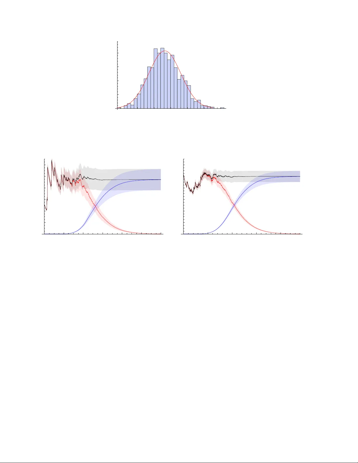
Mon. Not. R. Astron. Soc. 000 , 000–000 (0000) Printed 27 March 2022 (MN L A T E X style file v2.2) On statistical uncertain t y in nested sampling Charles R. Keeton Dep artment of Physics and Astr onomy, Rutgers University, 136 F r elinghuysen R oad, Pisc ataway, NJ 08854 USA 27 March 2022 ABSTRA CT Nested sampling has emerged as a v aluable tool for Ba yesian analysis, in particular for determining the Ba yesian evidence. The metho d is based on a sp ecific type of random sampling of the likelihoo d function and prior volume of the parameter space. I study the statistical uncertaint y in the evidence computed with nested sampling. I examine the uncertain t y estimator from Skilling (2004, 2006) and in tro duce a new estimator based on a detailed analysis of the statistical properties of nested sampling. Both p erform well in test cases and mak e it p ossible to obtain the statistical uncertaint y in the evidence with no additional computational cost. 1 INTR ODUCTION Ba yesian statistics pro vide a general framework for confronting mo dels with data (e.g., Gelman et al. 1995). Constraints on mo del parameters are quan tified by the p osterior distribution for the parameters given the data. The ov erall quality of a mo del is characterised by an in tegral o ver the p osterior, whic h is known as the evidenc e . The Bay esian evidence is esp ecially v aluable as an ob jective means of comparing models with different num b ers of parameters. The c hallenge with Ba yesian statistics is finding an efficient method to explore the posterior and/or compute the evidence. The p osterior may o ccup y many dimensions and hav e a complicated (and p ossibly multi-modal) shap e. Marko v Chain Monte Carlo (MCMC) methods hav e b ecome p opular as a wa y to generate samples of p oints drawn from arbitrary p osteriors (e.g., Gelman et al. 1995). MCMC samples are great for inferring parameter v alues and ranges, but they cannot be used by themselv es to ev aluate the evidence. MCMC methods can b e extended to yield the evidence via thermodynamic integration (see Gelman & Meng 1998, and references therein), but that approach can b e computationally intensiv e. Skilling (2004, 2006) recently in tro duced an approach called nested sampling that is sp ecifically designed to compute the Ba yesian evidence. Roughly sp eaking, the idea is to peel aw ay lay ers of constan t likelihoo d one b y one, and combine the lik eliho od v alues with the v olumes of the lay ers to obtain the evidence. The volumes may b e difficult to determine, but they can be estimated statistically if the likelihoo d lay ers are chosen in a particular wa y (see § 2.1 for details). While the analysis fo cuses on the evidence, it can yield a set of p oin ts drawn from the p osterior as a natural by-product. There are tw o practical challenges with nested sampling. The first is that at each step we need to generate a new point dra wn from the region inside an iso-lik eliho o d surface. A lot of the literature on nested sampling addresses methods for picking new points. Mukherjee et al. (2006) discuss dra wing points inside a multi-dimensional ellipsoid that encloses the lik eliho o d surface at L 0 , and ignoring any that hav e L < L 0 . Shaw et al. (2007), F eroz & Hobson (2008), and F eroz et al. (2009) develop metho ds that use multiple ellipsoids to handle more complicated likelihoo d functions, including multi-modal distributions. Chopin & Rob ert (2008) p oint out that imp ortance sampling can b e p o werful if one can find a distribution that is easy to dra w from and appro ximates the likelihoo d distribution mo derately well. Betancourt (2010) advocates using constrained Hamiltonian Monte Carlo metho ds to evolv e a new point from one of the kno wn points. All of those metho ds keep the core approac h of p eeling aw ay likelihoo d lay ers in sequence from the outside in, and differ only in the details of picking new points. Brew er et al. (2009) in tro duce a v ariant they call diffusive nested sampling that do es not alw ays require the steps to pro ceed from the outside in. The second challenge is that nested sampling, like any sto chastic sampling pro cedure, has some statistical uncertaint y in its results. General pro ofs establish that nested sampling conv erges to the correct evidence with an error that scales as N − 1 / 2 where N is a measure of the computational effort (Chopin & Robert 2008; Skilling 2009). How ever, in practical applications it would b e nice to ha ve a sp ecific estimate of the statistical uncertain ty in the evidence. That is the purpose of this pap er. I first review the nested sampling pro cedure ( § 2.1) and a p opular estimator from Skilling (2004, 2006) for the statistical uncertain ty in the evidence ( § 2.2). I then in tro duce a new uncertaint y estimator based on an analysis of the statistical c  0000 RAS 2 Ke eton prop erties of the nested sampling pro cedure ( §§ 2.3 and 2.4). I use n umerical tests to assess the estimators and provide some guidelines for c ho osing parameters that control the n umber of samplings ( § 3). The results presen ted here are applicable to an y implementation of nested sampling that uses the con ven tional approac h of p eeling aw ay likelihoo d lay ers in one direction only (i.e., to all curren t methods other than diffusiv e nested sampling). 2 THEORETICAL FRAMEW ORK 2.1 Nested sampling T o establish the concepts and notation, it is useful to review the nested sampling algorithm (see Skilling 2004, 2006 for details). Consider a likelihoo d function L ( θ ) defined on a parameter space θ , whic h ma y be m ulti-dimensional. 1 Priors on the parameters are sp ecified by π ( θ ), which is normalised such that R π ( θ ) dθ = 1. With simple flat priors, π ( θ ) = 1 /V where V is the v olume spanned by the allow ed range of parameters, but the framework can incorp orate non-flat priors as w ell. The Ba yesian evidence is then Z = Z L ( θ ) π ( θ ) dθ (1) Define a function X ( L ) to b e the fraction of the prior volume that lies at a likelihoo d lev el higher than L : X ( L ) = Z L ( θ ) >L π ( θ ) dθ (2) This is a monotonic decreasing function, with X (0) = 1. In principle, we can inv ert to find L ( X ) and then rewrite eq. (1) as Z = Z 1 0 L ( X ) dX (3) No w supp ose we can generate a sample of N nest p oin ts { L i , X i } suc h that the likelihoo d increases while the fractional volume decreases with the index i ; in other words, L i > L i − 1 and X i < X i − 1 , and we can consider L 0 = 0 and X 0 = 1. Then we can discretise the integral to estimate the evidence as Z = N nest X i =1 L i ( X i − 1 − X i ) (4) Later it will b e useful to consider the buildup of evidence by examining the “partial evidence” due to the contribution from the first k steps: Z k = k X i =1 L i ( X i − 1 − X i ) (5) There is some error in eq. (4) asso ciated with appro ximating the in tegral as a sum, but it is generally small compared with the statistical uncertaint y (Skilling 2006). There is also some error induced by truncating the sum, which is discussed in § 2.4. The heart of nested sampling is the method for generating the likelihoo d sampling { L i } and volume sampling { X i } . The idea is that it is (relativ ely) straightforw ard to pro duce a relev an t likelihoo d sampling, but it can b e difficult to determine the asso ciated volumes so we treat those statistically . Consider some likelihoo d threshold L 0 enclosing a volume V 0 . Supp ose w e hav e M p oints dra wn uniformly from that volume. In general there will be some (slightly) higher likelihoo d threshold L 1 > L 0 that encloses all M p oin ts. Statistically sp eaking, we can estimate the smaller enclosed v olume as V 1 = V 0 t 1 where t 1 is the largest of M random n umbers dra wn uniformly b etw een 0 and 1. In other words, t 1 is drawn from the probability distribution for the largest of M uniform deviates b etw een 0 and 1, which is p ( t ) = M t M − 1 for t ∈ [0 , 1] (6) W e can generalise to non-uniform priors b y defining the “volumes” to be integrals of the priors o ver the relev ant regions and ha ving the M p oin ts drawn from the prior distribution. The probabilit y distribution for t 1 remains unchanged. That idea leads to the follo wing pro cedure. Begin with M points—kno wn as “live” points—dra wn uniformly from the full prior distribution. Let the likelihoo ds of the live p oints b e L µ for µ = 1 , . . . , M . Then at step k of the nested sampling: (i) Extract the low est likelihoo d live p oin t and call it the k -th sampled point: L k = min( L µ ). (ii) Estimate the asso ciated volume as X k = X k − 1 t k (7) where t k is a random num b er drawn from p ( t ) in eq. (6). (iii) Replace the extracted live point with a new p oint that is drawn from the priors but restricted to the region L ( θ ) > L k . 1 T o simplify the notation, I do not explicitly indicate vectors or write the data dep endence in the likelihoo d function. c  0000 RAS, MNRAS 000 , 000–000 Statistic al unc ertainty in neste d sampling 3 Iterating this pro cess for a total of N nest steps yields a likelihoo d sampling { L i } and volume sampling { X i } that can b e com bined using eq. (4) to estimate the evidence. This is the conv entional nested sampling technique as defined b y Skilling (2004, 2006). The v arious implementations of nested sampling mainly differ in the wa y they find the replacement point in step (iii). 2.2 Skilling’s error analysis T o estimate the statistical uncertaint y asso ciated with sto chastic sampling, Skilling (2004, 2006) inv okes information theory . In general the p osterior p ( θ ) is (muc h) narro wer than the prior π ( θ ), and we can c haracterise the difference in terms of the “information gain” (also known as the Kullback-Leibler divergence; see Kullback 1959) H = Z p ( θ ) ln p ( θ ) π ( θ ) dθ (8) By Ba yes’s theorem, p ( θ ) = L ( θ ) π ( θ ) / Z so w e can write H = 1 Z Z L ( θ ) π ( θ ) ln L ( θ ) Z dθ = 1 Z Z L ( X ) ln L ( X ) dX − ln Z (9) using the same change of v ariables as in eq. (3). This integral can be discretised just like the evidence integral, so it is straigh tforward to estimate H from a given sampling { L i , X i } . Skilling (2004, 2006) argues that the num b er of steps needed to reach the p osterior is approximately H M where M is the n umber of liv e p oin ts, and that the dominant statistical uncertain ty arises from Poisson fluctuations √ H M in the num b er of steps. Thus, he estimates an uncertaint y in ln Z of ab out p H/ M . Note that Skilling argues that ln Z , and not Z itself, is the quan tity likely to hav e a fairly symmetric and quasi-Gaussian distribution. How ev er, if the uncertaint y is small (specifically , σ Z / Z  1), then Z itself will also b e Gaussian distributed and Skilling’s estimate corresp onds to a fractional uncertaint y in the evidence of σ Z Z ≈ r H M (10) This estimator is often used in nested sampling applications, but its accuracy has not (to my knowledge) b een rigorously established. 2.3 Momen t-based error analysis Skilling (2006) mentions that it should b e possible to obtain a more detailed estimate of the statistical uncertain ty b y computing the mean and v ariance of Z ov er all p ossible realisations of the volume sampling { X i } , but he do es not carry out the analysis. The goal of this section is to compute h Z i and  Z 2  to obtain a new estimator for σ Z . Since this estimator is based on the standard deviation, it is most useful when Z is Gaussian distributed, i.e., when the uncertain ties are small ( σ Z / Z  1). This do es not seem like a significant limitation, though, b ecause in man y applications it will b e desirable to ac hieve small uncertain ties. It is conv enient to use eq. (7) to write the v olumes as X i = i Y j =1 t j (11) The adv antage is that the X i ’s are statistically correlated, but the t i ’s are indep endent and that allows us to decomp ose the join t probabilit y density for all the t i ’s in to a pro duct: p all ( t 1 , t 2 , t 3 , . . . ) = p ( t 1 ) p ( t 2 ) p ( t 3 ) · · · (12) where p ( t ) is from eq. (6). W e can then write the av erage of any quantit y f ov er all realisations of the volume sampling as h f i ≡ Z f ( t 1 , t 2 , t 3 , . . . ) p ( t 1 ) p ( t 2 ) p ( t 3 ) · · · dt 1 dt 2 dt 3 · · · (13) It is imp ortan t to understand that such an av erage only spans the volume sampling; at this point we are not considering differen t realisations of the likelihoo d sampling. As part of this analysis w e need moments of the t probability distribution, h t n i = Z 1 0 t n p ( t ) dt = M M + n (14) Com bining eqs. (4) and (11), w e can write the (partial) evidence in terms of the t i ’s as Z k = k X i =1 L i (1 − t i ) i − 1 Y j =1 t j = k X i =1 L i i − 1 Y j =1 t j − i Y j =1 t j ! (15) c  0000 RAS, MNRAS 000 , 000–000 4 Ke eton Since the terms in the pro ducts are statistically indep endent, we can factorise the av erage of a pro duct and write * n Y j =1 t j + = n Y j =1 h t j i = h t i n (16) for an y n ∈ [1 , N nest ]. This allows us to write the av erage of the evidence after any step k as h Z k i = * k X i =1 L i i − 1 Y j =1 t j − i Y j =1 t j !+ = k X i =1 L i  h t i i − 1 − h t i i  = 1 M k X i =1 L i h t i i = 1 M k X i =1 L i  M M + 1  i (17) This is a simple expression for the (partial) evidence av eraged ov er all possible realisations of the v olume sampling (giv en a particular likelihoo d sampling { L i } ). Ob viously the final evidence is obtained just b y ev aluating at k = N nest . T o compute the second moment it is conv enient to b egin with the partial evidence from eq. (5):  Z 2 k  = *" k X i =1 L i (1 − t i ) i − 1 Y j =1 t j #   k X i 0 =1 L i 0 (1 − t i 0 ) i 0 − 1 Y j 0 =1 t j 0   + =  Z 2 k − 1  + *" L k (1 − t k ) k − 1 Y j =1 t j # 2 + + 2 *" k − 1 X i =1 L i (1 − t i ) i − 1 Y j =1 t j #   L k (1 − t k ) k − 1 Y j 0 =1 t j 0   + (18) In the second line I separate the joint sum ov er i, i 0 6 k into three comp onents. The first comp onen t includes all terms with i, i 0 6 k − 1, so we can immediately recognise it as  Z 2 k − 1  . The second component is the term with i = i 0 = k . The third comp onen t includes all terms in which one index equals k while the other runs o ver v alues 6 k − 1. Since we can in terchange i and i 0 , there is a leading factor of 2. It takes a few steps to ev aluate the av erages. First consider the second term in eq. (18). W riting out the products of t i ’s and collecting terms yields * L 2 k k − 1 Y j =1 t 2 j − 2 t k k − 1 Y j =1 t 2 j + k Y j =1 t 2 j !+ = L 2 k   t 2  k − 1 − 2 h t i  t 2  k − 1 +  t 2  k  = 2 M ( M + 1) L 2 k  t 2  k (19) No w consider the third term in eq. (18). W e can rewrite the pro ducts, taking care to distinguish the t ’s that app ear t wice in a product from those that app ear just once, and thus obtain * 2 L k k − 1 X i =1 L i   i − 1 Y j =1 t 2 j k − 1 Y j 0 = i t j 0 − i Y j =1 t 2 j k − 1 Y j 0 = i +1 t j 0 − i − 1 Y j =1 t 2 j k Y j 0 = i t j 0 + i Y j =1 t 2 j k Y j 0 = i +1 t j 0   + = 2 L k k − 1 X i =1 L i   t 2  i − 1 h t i k − i −  t 2  i h t i k − i − 1 −  t 2  i − 1 h t i k − i +1 +  t 2  i h t i k − i  = 2 M ( M + 1) L k h t i k k − 1 X i =1 L i  t 2  i h t i i (20) Notice that eq. (19) has the same form as each term in the sum in eq. (20), but with index i = k . So when w e insert eqs. (19) and (20) back into eq. (18), w e can write  Z 2 k  =  Z 2 k − 1  + 2 M ( M + 1) L k h t i k k X i =1 L i  t 2  i h t i i (21) With this expression for the second momen t of the partial evidence, we see that the second moment of the full evidence can b e written as  Z 2  = 2 M ( M + 1) N nest X k =1 L k h t i k k X i =1 L i  t 2  i h t i i = 2 M ( M + 1) N nest X k =1 L k  M M + 1  k k X i =1 L i  M + 1 M + 2  i (22) Com bining eqs. (17) and (22) in the usual wa y yields a new estimator for the statistical uncertaint y in the evidence: σ 2 Z = 2 M ( M + 1) N nest X k =1 L k  M M + 1  k k X i =1 L i  M + 1 M + 2  i − 1 M 2 " N nest X i =1 L i  M M + 1  i # 2 (23) F or comparison, rewriting eq. (10) in the current notation yields the following expression for Skilling’s uncertaint y estimator: σ 2 Z = 1 M 3 " N nest X i =1 L i  M M + 1  i # " N nest X j =1 L j ln L j  M M + 1  j # − 1 M 3 " N nest X i =1 L i  M M + 1  i # 2 ln " 1 M N nest X j =1 L j  M M + 1  j # (24) On the surface these t wo expressions look quite different, so it is interesting to compare them in quantitativ e examples. c  0000 RAS, MNRAS 000 , 000–000 Statistic al unc ertainty in neste d sampling 5 2.4 Handling the remainder When the nested sampling pro cedure is complete, there is some (small) remaining volume, X N nest , whose contribution to the evidence is neglected in eq. (4). While w e can mak e its con tribution arbitrarily small by taking enough steps (see § 3.4), w e can also include it at the exp ense of making the analytic expressions slightly more complicated. Supp ose we truncate nested sampling after step k and compute the partial “nested evidence” Z k from eq. (5). W e can estimate the remaining evidence as a pro duct of the remaining volume, X k , and the mean likelihoo d within that v olume. Since the live p oints are dra wn uniformly from X k , w e can estimate the mean likelihoo d from the live p oin ts as ¯ L ( k ) = 1 M M X µ =1 L µ (25) Here the o verbar distinguishes this a verage ov er live p oin ts from an av erage o ver volume realisations, and the superscript is a reminder that the a verage is tak en after step k . Thus the “live evidence” is Z live k = ¯ L ( k ) X k (26) Av eraging the live evidence ov er all v olume realisations yields D Z live k E = ¯ L ( k ) h X k i = ¯ L ( k ) * k Y j =1 t j + = ¯ L ( k )  M M + 1  k (27) The second moment is D ( Z live k ) 2 E = ( ¯ L ( k ) ) 2  X 2 k  = ( ¯ L ( k ) ) 2 * k Y j =1 t 2 j + = ( ¯ L ( k ) ) 2  M M + 2  k (28) so the statistical uncertaint y in the live evidence is σ 2 Z live k = ( ¯ L ( k ) ) 2  M M + 1  k "  M + 1 M + 2  k −  M M + 1  k # (29) No w consider the estimate of the total evidence after step k , Z tot k = Z k + Z live k (30) The av erage o ver volume realisations is simply obtained from eqs. (17) and (27). The statistical uncertain ty in Z tot k is σ 2 Z tot k = σ 2 Z k + σ 2 Z live k + 2 D Z k Z live k E − h Z k i D Z live k E (31) The term in parentheses accounts for the fact that Z live k and Z k are not indep enden t b ecause they b oth inv olve the same v olume sampling. The cross term can b e ev aluated using an analysis similar to that in eq. (20), which yields D Z k Z live k E = ¯ L ( k ) M + 1  M M + 1  k k X i =1 L i  M + 1 M + 2  i (32) Putting the pieces together, w e find that including the liv e evidence increases the statistical uncertaint y in the total evidence according to σ 2 Z tot k = σ 2 Z k + ∆ σ 2 Z k (33) where the original uncertaint y is giv en in eq. (23) while the increase is ∆ σ 2 Z k = ( ¯ L ( k ) ) 2  M M + 1  k "  M + 1 M + 2  k −  M M + 1  k # + 2 ¯ L ( k )  M M + 1  k k X i =1 L i " 1 M + 1  M + 1 M + 2  i − 1 M  M M + 1  i # (34) In the examples that follow, I take enough steps that the liv e evidence pro vides a negligible contribution by the end, but the formalism in this section can b e used if the num b er of nested sampling steps is more mo dest. 3 NUMERICAL RESUL TS In this section I present numerical tests designed to assess the uncertaint y estimators, and to inv estigate how man y samples to use. Since the nested sampling framework do es not require an y sp ecific assumptions ab out the form of the likelihoo d distribution, a Gaussian test case should b e sufficien t. How ever, I also consider a log-normal distribution as a chec k. c  0000 RAS, MNRAS 000 , 000–000 6 Ke eton 0.7 0.8 0.9 1.0 1.1 1.2 V Z 1 2 3 4 5 probability Figure 1. The histogram shows the distribution of evidence v alues (specifically V Z ) for 1000 realisations of the volume sampling, given a particular likelihoo d sampling. The red curve shows a Gaussian distribution whose mean and varaiance are computed from eqs. (17) and (23). The mean and standard deviation from the simulations are 0 . 878 ± 0 . 084 (the mean differs from V Z ≈ 1 for this particular likelihood sampling). F or comparison, the analytic av erage ov er volume realisations is 0.883, and Skilling’s and m y uncertaint y estimators yield 0.083 and 0.085, respectively . 3.1 Gaussian test case Consider a m ultiv ariate Gaussian likelihoo d sp ecified by some mean vector and co v ariance matrix. With flat priors we can mak e the following simplifications. Choose co ordinates centred on the mean and aligned with the principal axes of the cov ariance matrix. Scale each co ordinate b y the standard deviation in that direction. This yields a multiv ariate Gaussian in canonical form, L ( θ ) = (2 π ) − d/ 2 e −| θ | 2 / 2 (35) where d is the num b er of dimensions. Let the prior v olume b e a cub e of side length s centred on the origin, so the prior v olume is V = s d and the priors are π ( θ ) = 1 /V . Th us the evidence is Z = V − 1 Z V (2 π ) − d/ 2 e −| θ | 2 / 2 dθ (36) If the prior b ox is large enough to encompass essentially all of the likelihoo d, then V Z ≈ 1 indep endent of the b ox size. F or this reason, in the follo wing tests I examine V Z instead of just Z . The information gain for this case is H = 1 V Z Z L ln L Z dθ ≈ − d 2 (1 + ln 2 π ) − ln Z (37) In the last step I again assume the prior b ox is large. F or concreteness, I use a b ox with side length s = 10 in d = 4 dimensions; these choices influence the quantitativ e details but do not affect the general conclusions. In the fiducial case I use M = 400 liv e p oin ts and tak e N nest = 4100 steps (see § 3.4). The asso ciated information gain is H = 3 . 53, and Skilling’s estimator of the fractional uncertain ty in the evidence has an analytic v alue of p H/ M = 0 . 094. 3.2 T esting the volume sampling I first generate a single realisation of the lik eliho o d sampling and com bine it with 1000 realisations of the volume sampling. Figure 1 sho ws a histogram of the V Z v alues from these direct sim ulations. The mean and standard deviation of the sim ulated v alues are 0 . 878 ± 0 . 084. The mean differs from the theoretical v alue V Z ≈ 1 b y ab out 1 . 5 σ for this particular realisation of the likelihoo d sampling. F rom eq. (17) the predicted av erage ov er volume realisations is 0.883. Skilling’s estimator yields a statistical uncertaint y of 0.083, while mine yields 0.085. The predicted Gaussian distribution agrees w ell with the simulation results, indicating that Z has a (nearly) Gaussian distribution when the uncertain ties are small (qv. §§ 2.2 and 2.3). I conclude that the analytic expressions accurately describ e the distribution of evidence v alues for many realisations of the volume sampling. It is striking that the tw o uncertaint y estimators yield very similar v alues despite ha ving such different analytic forms. 3.3 T esting the likelihoo d sampling It is useful to see how the results v ary with different realisations of the likelihoo d sampling. I now generate 1000 random lik eliho od samplings; for eac h one I compute the mean evidence a veraged ov er all v olume samplings using eq. (17). Figure 2 sho ws a histogram of the v alues of h V Z i t for the different likelihoo d realisations (I add the subscript t to emphasise that the c  0000 RAS, MNRAS 000 , 000–000 Statistic al unc ertainty in neste d sampling 7 0.8 0.9 1.0 1.1 1.2 1.3 < VZ > t 1 2 3 4 probability Figure 2. The histogram sho ws the distribution of h V Z i t for 1000 realisations of the lik eliho o d sampling. The notation h V Z i t emphasises that I a verage o ver all volume samplings for each likelihoo d sampling. The red curv e sho ws a Gaussian distribution whose mean and v ariance are computed from eqs. (17) and (23). The mean ov er all likelihoo d samplings is 1.005; the empirical scatter in the histogram is 0.094, while the predicted v alue is 0.094 for Skilling’s estimator and 0.096 for mine. 0 200 400 600 800 1000 1200 step 0.2 0.4 0.6 0.8 1.0 1.2 V Z 0 1000 2000 3000 4000 step 0.2 0.4 0.6 0.8 1.0 1.2 V Z Figure 3. Developmen t of the evidence as a function of step index. The blue band sho ws the mean and 1 σ errors for the “nested evidence” (eqs. 17 and 23), the red band sho ws the “live evidence” (eqs. 27 and 29), and the black curve sho ws the total (eqs. 30 and 33). The num b er of live p oin ts is M = 100 (left) and M = 400 (right). With more live p oints, it takes more steps to reach conv ergence, but the ultimate uncertaint y is smaller. a verage is ov er volume samplings). The mean and standard deviation for the histogram are 1 . 005 ± 0 . 094. On a verage, nested sampling recov ers the evidence very well. Strictly sp eaking, both of the uncertaint y estimators depend on the lik eliho o d sampling, but the scatter across the lik eliho od realisations is < 9% so any single case provides a useful v alue. The av erage predicted uncertaint y is 0.094 for Skilling’s estimator, and 0.096 for mine. Also, the predicted Gaussian distribution agrees well with the empirical histogram. I conclude that the b oth analytic estimators characterise the statistical uncertaint y in the evidence quite well. It is not obvious at this p oint why the t wo uncertaint y estimators yield suc h similar results. 3.4 Ho w many live points and steps? Let us now consider how to c ho ose the num b er of live p oin ts, M , and the num b er of nested sampling steps, N nest . One general goal is to hav e nested sampling “find” all significan t mo des in the p osterior. The sampling pro cedure is basically guaranteed to find the p eak for a unimo dal distribution, but if the live p oin ts are to o sparse they may miss some peaks (esp ecially small ones) in a m ulti-mo del distribution. In order to ha ve a reasonable probability of getting at least one live point in each mode at the outset, F eroz & Hobson (2008) suggest that the n umber of liv e points should exceed V prior /V min , where V prior is the v olume spanned by the priors while V min is the volume of the smallest mode (which m ust b e estimated since it cannot actually b e known b efore the analysis is done). The second consideration relates to ac hieving a robust and precise estimate of the evidence. Figure 3 sho ws the dev el- opmen t of the evidence as a function of the step index, for tw o c hoices of M . After some n umber of steps the evidence and uncertain ty saturate in the sense that taking additional steps do es not significantly change the results. F or a heuristic under- standing, note that as nested sampling homes in on a lik eliho o d peak the likelihoo d v alues b ecome constan t ( L i → L peak ) while the volumes b ecome progressiv ely smaller ( X i → 0). F or a rigorous pro of of conv ergence, see Skilling (2009). c  0000 RAS, MNRAS 000 , 000–000 8 Ke eton 1000 2000 3000 4000 5000 6000 7000 N tot 0.05 0.10 0.15 0.20 Σ  Z Figure 4. The points show the fractional uncertain ty in the evidence v ersus the total n umber of lik eliho od ev aluations ( N tot = N nest + M ) for tests in which the num b er of liv e points is M = 100 , 200 , 300 , 400 , 500 , 600 (left to right). Here N nest is determined for each M using the stopping threshold  = 0 . 01. The curve shows the scaling relation σ Z / Z ∝ N − 1 / 2 tot . The question arises of how to iden tify the p oint of diminishing returns. One simple possibility (Skilling 2004, 2006) is to compare the evidence accumulated through nested sampling ( Z k from eq. 5) with the remaining evidence estimated from the live p oints ( Z live k from eq. 26). Figure 3 shows Z live k v ersus k in red. A t early stages the curve sho ws a series of spik es: it rises sharply when a new live point is found that (temp orarily) dominates the av erage o ver live p oin ts, then declines as the v olume decreases. The curve smo othes out as the liv e points come to hav e more similar lik eliho ods, and then deca ys as the lik eliho ods saturate while the remaining volume contin ues to decrease. Roughly sp eaking, Z live represen ts the evidence that has been “missed” by the nested sampling pro cedure, so we may wan t to contin ue the nested sampling until the ratio of live to nested evidence falls b elo w some threshold: Z live / Z <  . Figure 3 illustrates that using more live p oin ts means it takes more steps to reac h a given  threshold, but the extra computational effort is rew arded with a smaller statistical uncertaint y . It is therefore interesting to compare the achiev ed uncertain ty with the computational effort, which we may measure as the total num b er of likelihoo d samples ( N tot = N nest + M ). Figure 4 shows this comparison for different num b ers of live p oin ts, giv en a fixed stopping threshold  = 0 . 01. The fractional uncertain ty clearly decreases with the total num b er of samples as σ Z / Z ∝ N − 1 / 2 tot , just as expected for a statistical sampling pro cedure (Skilling 2004, 2006; Chopin & Rob ert 2008). In the examples presented here, I ha ve used a lo w  threshold to require that the live evidence b e negligible at the end of the run. Figure 3 suggests, how ever, that  could b e set higher pro vided that the live evidence is accounted for prop erly (using the metho ds in § 2.4). The lessons here are familiar from previous work on nested sampling, but worth reiterating. The ultimate statistical uncertain ty dep ends mainly on the n umber of liv e p oints. Once the nested sampling procedure has con verged (as measured, for example, by the  threshold), running more steps will not improv e the results. The wa y to reduce the uncertainties is to increase the n umber of live points. 2 That will increase the n umber of steps it takes to reach con vergence, but will yield uncertain ties that scale as σ Z ∝ N − 1 / 2 tot . 3.5 Log-normal test case No where in the theoretical framew ork was it necessary to sp ecify the form of the likelihoo d, so the Gaussian test case should b e sufficien t to v alidate the analytic results. Nevertheless, it is useful to consider a differen t test to verify that the results are indeed robust. I use a m ultiv ariate log-normal distribution because it is sk ewed and non-Gaussian but still analytically tractable. Cho osing appropriate scaled co ordinates, w e can write the likelihoo d in canonical form, L ( θ ) = d Y i =1 e − (ln θ i ) 2 / 2 (2 π ) 1 / 2 θ i (38) where d is the n umber of dimensions. Let the prior volume b e the cub e with 0 < θ i < s , so V = s d and the evidence is Z = V − 1 d Y i =1 Z s 0 e − (ln θ i ) 2 / 2 (2 π ) 1 / 2 θ i dθ i (39) 2 It is not necessary to start from scratch in order to increase the num b er of live p oints. Skilling (2006) explains that indep enden t runs with M 1 , M 2 , . . . live p oints can b e merged into a joint run that effectiv ely has M 1 + M 2 + . . . live p oints. The likelihoo d samplings are simply merged and sorted, while the volume sampling must be recomputed. c  0000 RAS, MNRAS 000 , 000–000 Statistic al unc ertainty in neste d sampling 9 F or a large prior b o x, V Z ≈ 1 and the information gain is H = 1 V Z Z L ln L Z dθ ≈ − d 2 (1 + ln 2 π ) − ln Z (40) I again w ork in d = 4 dimensions, but no w use a b o x with s = 20 to encompass the bulk of the lik eliho o d. Given the larger v olume, I use M = 600 liv es points and tak e N nest = 9000 steps. F or these parameter c hoices, the information gain is H = 6 . 31 and Sk illing’s estimator for the fractional uncertaint y in the evidence has an analytic v alue of p H/ M = 0 . 103. I first consider a single likelihoo d sampling and examine the distribution of evidence v alues for 1000 v olume realisations (qv. § 3.2). The empirical mean and standard deviation ov er the volume samplings are 0 . 939 ± 0 . 097. The analytic mean is 0.944, while Skilling’s and m y estimators predict uncertainties of 0.097 and 0.098, resp ectively . The histogram of Z v alues (not shown) agrees well with a Gaussian distribution whose mean and v ariance are giv en b y eqs. (17) and (23). (Note that Z can ha ve a nearly-Gaussian distribution ev en if the lik eliho o d is non-Gaussian.) I next consider 1000 likelihoo d samplings and examine the distribution of h V Z i t v alues (qv. § 3.3). The empirical mean and standard deviation are 0 . 997 ± 0 . 106. Skilling’s and my estimators predict uncertainties of 0.102 and 0.103, resp ectiv ely . The histogram of h V Z i t again agrees w ell with the predicted Gaussian distribution. I conclude that the analytic results are reliable even for a non-Gaussian lik eliho od distribution. 4 SUMMAR Y I ha ve derived simple analytic expressions for the mean and v ariance of the Ba yesian evidence ov er all realisations of the v olume sampling in nested sampling, and compared them with the uncertain ty estimator in tro duced by Skilling (2004, 2006) from an information theoretic argument. The tw o estimators hav e differen t forms as sums ov er the likelihoo d sampling, y et they yield v ery similar quan titative results. A t this point it is not clear whether the agreement reflects some general equiv alence b et ween the tw o estimators that is not yet apparen t, or whether it somehow depends on statistical prop erties of the likelihoo d sampling { L i } that emerges from the nested sampling pro cedure. The moments-based estimator curren tly has a more rigorous foundation than the information theoretic estimator, but b oth are useful and it will be interesting to see if they contin ue to give similar results as nested sampling is applied to a broader range of problems, and if any formal equiv alence can b e established. Both estimators can b e used to compute the statistical uncertaint y in the evidence for an y implemen tation that main tains the core prescription of nested sampling: each new point is drawn from the prior distribution in the region inside the current likelihoo d surface. With these results, determining not only the mean evidence but also the uncertaint y requires no additional computational effort (and no guesswork) b ey ond that needed to generate the likelihoo d sampling. A CKNOWLEDGMENTS I thank Ross F adely for v aluable discussions ab out nested sampling, and the referee for suggesting the error analysis in § 2.4. This w ork received supp ort from the US National Science F oundation through gran t AST-0747311. REFERENCES Betancourt M. J., 2010, e-prin t Brew er B. J., P´ arta y L. B., Cs´ an yi G., 2009, e-print Chopin N., Rob ert C., 2008, e-print F eroz F., Hobson M. P ., 2008, MNRAS, 384, 449 F eroz F., Hobson M. P ., Bridges M., 2009, MNRAS, 398, 1601 Gelman A., Meng X.-L., 1998, Statistical Science, 13, 163 Gelman A. B., Carlin J. S., Stern H. S., Rubin D. B., 1995, Bay esian Data Analysis. Chapman & Hall/CR C, Bo ca Raton Kullbac k S., 1959, Information Theory and Statistics. John Wiley and Sons, NY Mukherjee P ., Parkinson D., Liddle A. R., 2006, ApJ, 638, L51 Sha w J. R., Bridges M., Hobson M. P ., 2007, MNRAS, 378, 1365 Skilling J., 2004, in American Institute of Ph ysics Conference Series, V ol. 735, American Institute of Physics Conference Series, R. Fischer, R. Preuss, & U. V. T oussaint, ed., pp. 395–405 —, 2006, Bay esian Analysis, 1, 833 —, 2009, in American Institute of Physics Conference Series, V ol. 1193, American Institute of Physics Conference Series, P . M. Goggans & C.-Y. Chan, ed., pp. 277–291 c  0000 RAS, MNRAS 000 , 000–000