Multiple-Campaign Ad-Targeting Deployment: Parallel Response Modeling, Calibration and Scoring Without Personal User Information

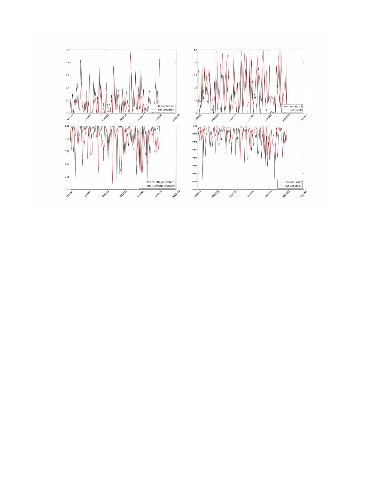
Multiple-Campaign Ad-T ar geting Deployment P arallel Response Modeling, Calibration and Scor ing Without P ersonal User Inf or mation P aolo D’Alber to NinthDecimal pdalberto@ninthdecimal.com ABSTRA CT W e present a vertical introduction to campaign optimization: we want the ability to predict any user response to an ad campaign without any users’ profiles on an av erage and for each exposed ad, we want to provide of fline modeling and validation, and we want to deploy dedicated hardware for on-line scoring. In prac- tice, we present an approach how to build a polytomous model (i.e., multi response model) composed by sev eral hundred binary models using generalized linear models. The theory has been intro- duced twenty years ago and it has been applied in dif ferent fields since then. Here, we sho w how we can optimize hundreds of cam- paigns and how this large number of campaigns may overcome a few characteristic caveats of single campaign optimization. W e dis- cuss the problem and solution of training and calibration at scale. W e present statistical performance as covera ge , pr ecision and r e- call used in off line classification. W e present also a discussion about the potential performance as throughput for on-line scoring: how many decisions can be done per second streaming the bid auc- tions also by using dedicated hardware such as Intel Phi. Categories and Subject Descriptors H.3.5 [ Information Storage and Retriev al ]: Online Information Services; G.4 [ Mathematical software ]: Parallel and vector im- plementations K eywords Algorithms 1. INTR ODUCTION Free contents and targeted advertising are Janus-faces; that is, the beginning and the end of a cycle. W e start by w atching original contents and e xposing our likes to the contents providers. In turn, our preferences are used to provide audience tar geting for advertis- ers, which at the end of the day pay for the contents. W e would like that the advertising should be tailored to the au- dience in such a way that the ads are relevant, engaging, and with Permission to make digital or hard copies of all or part of this work for personal or classroom use is granted without fee provided that copies are not made or distrib uted for profit or commercial adv antage and that copies bear this notice and the full citation on the first page. T o copy otherwise, to republish, to post on servers or to redistrib ute to lists, requires prior specific permission and/or a fee. Copyright 20XX A CM X-XXXXX-XX-X/XX/XX ...$15.00. high precision in order to minimize the costs and to maximize the return to the original in vestment. Collecting personal history is a common approach used to un- derstand the audience and to find ways to reach them. Every time we log into our mail account(s), social network(s), search(es) and for anything we do afterwards, these events help describing who we are and what we do. These profiles attract a large spectrum of interests as the like of advertisers, recruiters, prospects, or at worst soliciting email. Considering that a social network can reach billions of people, collecting and classifying these volume of data is not an easy chore. Nonetheless, the classification changes little in time. For example, we like Italian Opera and we will, likely , for life; other likes may be more flaky . Now let us put the previous problem in the context of avail ads. For example, there are ad-exchanges where an ad-compan y can go, bid, and buy impressions (ad-space): by counting the largest ex- changes, we could bid up to 10 Billions impressions e very day in US alone, reaching 150 Million people, say , and serving thousands of campaigns. If we deploy users’ profiles, we need to have in- formation only about the 150 Millions. If we do not hav e such information, we may have to make a new and a different decision for each impression: the problem space becomes larger and thus the problem harder (10 Billions). In practice, not e veryone wants to collect personal information and not ev ery one can or will be able to. One day , cookies associ- ated to browsers may be gone and thus the main mean to follow us is to log in (Google, Facebook and Y ahoo) or tracking the location of our devices (Geo location). In this work, we do not collect any personal information: we care about the collective and anonymous response. W e shall clarify what we collect in Section 5. The ne xt question will be ho w can we tailor the response of hun- dreds of campaigns? Campaigns are now being designed for an interaction with the audience: for example, clicking to redeem a coupon, responding to a trivia question, playing a game and others. These interactions set apart these impressions: campaigns and ad- vertisers want to respond to the feedback in order to focus more to who really show interests. Click Through Rate (CTR) is a measure of performance for a campaign. By construction, CTR is a ratio defined as the number of clicks over the total number of impressions deliv ered. Assume we reach all members of our audience and the people really inter- ested to the campaign clicked to their satisfaction. If we have to redo the same campaign, we would be parsimonious and reduce the number of impressions maintaining the same interests, same number of clicks, and thus larger CTR. Problem. For example, giv en an impression x , with its fea- tures from a pool of n impressions, we would like to compute the probability P C ` ( x ) of a click for the campaign C ` , where we have 1 ≤ ` ≤ N . In practice, we model this problem by estimating each binomial distribution: P C ` [ Y = k ] = n k ! p k C ` (1 − p C ` ) n − k , k ∈ [0 , n ] (1) W e are after the parameter p C ` , the average probability of a click, and its connection with the features x of the impression x ; that is, p C ` = g ( x ) . W e organize the paper as follo ws. In Section 2, we introduce the basic applied statistic method used to estimate the connection between any impression x and its probability as in Equation 1. In practice, we dwell with a problem that has a small number of pos- itiv e cases and a very large number of negati ve ones. In Section 3, we present our approach to select retrospective sampling, ex post , and in particular ho w to select the negati ve cases (no real ones) and how to scale to pro vide prospecti ve estimate, e x ante , which can be used for bidding in real time. W e e xplain also our approach to cali- brate the system and choose thresholds to mimic a binary response. In Section 5, we present how we explore the features space. In Section 6, we put everything together and we present measure of quality such a precision. Eventually , the computation of P C ` ( x ) has to be efficient and performed at run time; in Section 7.1, we provide throughput using state of the art systems. W e wrap up in Section 8 and we tip our hats to who helped us in Section 9. 2. GLM, GENERALIZED LINEAR MOD- ELS Suppose that we want to have a response Y i that can take only two possible values: Y i = 1 and Y i = 0 . For example, the for- mer represents the response of a click or success and the latter the response to a non click or failure. W e write P [ Y i = 0] = 1 − π i , P [ Y i = 1] = π i (2) W e describe this as Y i ∼ B (1 , π i ) . This is a single trial. If we hav e m independent trials, and there is a common probability π of success and probability 1 − π of f ailure, we say that Y ∼ B ( m, π ) and P [ Y = k ] =  m k  π k (1 − π ) n − k , for any integer 1 < k < m . The probability distribution is counting the number of k possible successes over a pool of m trials. The Binomial distribution is one of the oldest to be studied and it was derived by Jacob Bernoulli [1]. Our notations and references are from [3], Chapther 2. In general, we cannot assure homogeneity and we should con- sider a process such as Y = P m i =1 Y i where Y j ∼ B (1 , π j ) , that is the summation of non homogeneous Binomial. Also, the values of π 1 , . . . , π m are often unknown and we will ev entually compute an av erage Y i ∼ B (1 , π ) and Y ∼ B ( m, π ) where π = 1 m P m i =1 π i . It should be clear no w that Y is a response to an ev ent. The ev ent is represented by a vector of explanatory variables x = ( x 1 , . . . , x p ) . The principal objectiv e of a statistical analysis is to in vestigate the relationship between the response probability π and the explanatory x , that is to find g ( π ) ∼ x . What follows, especially the notations and the meaning behind the notation is from [6] Chapter 2 and 4. Linear models play an important role in applied and theoretical work. W e suppose there is a linear dependence g ( π i ) = η i = p X j =1 x i,j β j (3) for to be computed β 1 , . . . , β p . The function g () is a transforma- tion that makes possible to map the range [0 , 1] , which is the range of probability , to a more appropriate space ( −∞ , + ∞ ) , which is appropriate for a linear function. In this work we use the logistic function log e  π i 1 − π i  = β 0 + p X j =1 x i,j β j (4) where the fraction π i 1 − π i has range in the interv al [0 , + ∞ ) and it also know as odd ratio (e.g., used for hypothesis testing and se- quential analysis [7]). In Equation 4, we single out the parameter β 0 , which is the inter cept . As a note, the equation 4 is for ev ery trial and our ability of estimating π i howe ver the unknown β s are determined for all. There is also another and v ery important reason to use the logistic regression as we shall e xplain in Section 2.2. 2.1 Computing β : Maximum likelihood. The responses y 1 , . . . , y n = y are observed from the inde- pendent binomial v ariables Y 1 , . . . , Y n = Y such that Y i ∼ B ( m i , π i ) and we could use the e xpression Y ∼ B ( m , π ) . The log likelihood may be written as: l ( π , y ) = X i =1 [ y i log( π i 1 − π i ) + m i log(1 − π i )] (5) where we omit the term P log  m i y i  , which is a constant indepen- dent of π . If we substitute the linear logistic model in Equation 4 we hav e l ( β , y ) = X i X j y i x i,j β j − X i m i log(1 + e P j x i,j β j ) , (6) or in matrix form l ( β , y ) = y t X β − X i m i log(1 + e X t i β ) (7) W e identify with ˆ β the value of β that maximizes Equation 6. The appealing of this formulation is that log likelihood de- pends on y only through the linear combinations y t X and y t X = E [ Y t X ; ˆ β ] . The details of the computation of ˆ β are av ailable [6] Section 4.4.2. It is an iterative solver where at every iteration in- volv es a matrix factorization. The matrix factorization may be pro- hibitiv e as the matrix X will become larger . The iterative approach uses weights to giv e more importance to specific dimensions. The weight may adapt at each iterations and it may require a computation of a different QR matrix factorization. There are suggestions where the factorization can be done once and being reused (circumventing one of the most expensi ve step) because the weights will change the spectrum of R ∼ √ w t R but will not change the spectrum of Q , which must be a unitary matrix (e.g. [2] Chapter 5). 2.2 Ex P ost vs. Ex Ante: differ ent Inter cept. In [6] Section 4.3.3, there is a full explanation but this property should strike a chord to anyone using models for predictions. In general, we use the past responses (i.e., ex post) to compute ˆ β : W e consider the past clicks and non clicks for the impressions we hav e deliv ered. If we are in the process of completion we have not seen all clicks and, most importantly , we have not seen all impressions yet. As matter of fact, the pool of av ailable impressions is ev en larger than the one we are going to deli ver (i.e., ex ante). The ex-post b uilding model approach is practical. The ex ante is not. If we could build both they will differ only by their intercept β 0 . This is true because of logit canonical link in Equation 4. The difference can be computed if we hav e at least an estimate of the difference in scale of the ex-post (training) and ex-ante (total) sets. Notice that no other link function has such a property . This mathematical adjustment is simple to explain and to use. But it has an e ven more important ramification: if we have multiple models for different campaigns, then we can argue we can compare their probability estimates of success and choose accordingly based on their ex ante, which are more useful, instead of their ex post, which are too specific. It will become really a prediction and not just a classification. W e will come back to this subject in Section 6. 3. POSITIVE AND NEGA TIVE SET Events like clicks or any call to action are rare. If you consider the training set as the composition of positi ve ev ents and nega- tiv e events, the choice of positiv es is clearly defined. The choice and the quantity of ne gati ves is quite a different problem: clicks to other campaigns, non-clicked impressions b ut delivered to the same campaign, to other campaigns, and impressions that are not ev en selected for bidding. The list is long and the number of im- pression in it is very large. T o gi ve a quantitati ve measure, we may hav e 1 Million click, 3.5 Billion delivered impressions, and 2 Tril- lion av ailable impressions ev ery year . Common practice would be to choose 1 Million negati ves, but where to find these impressions and what are these impressions are very tricky questions: in prac- tice, the choice of the ne gati ve impression to use for training affects any model. At first, given a campaign and its clicks, say one thousand, we thought we could choose another one thousand from the delivered impressions. Then we could build a model ˜ β . Having the model, we could score all delivered impressions and create a distribution. Then we could bin the distribution in 100 bins and sample 10 im- pression per bin in order to find a second negati ve set. Then com- pute ˆ β . There is one practical problem: we need to score all impressions and this is just to retrieve a suitable sample as small as the number of clicks. From a practical point of view , we used clicked impressions only: Given an acti ve campaign from time t A to t B with t A < t B , we collected all its clicks, these are the positives. The clicks to the other campaigns in the same interval of time are the negati ves. In practice, we split the click space so that each model and campaign will bring forth its unique features and all may cov er the av ailable clicks. W e shall show the models so created will actually co ver this space. This is the training set upon we are going to build the model ˆ β . T raining and calibration shall be described in the following sec- tion. Once the model is built, we will have a better understanding what features are important and how they affect the model. Also, we may ha ve a clear understanding what features determine a clear rejection: Thus we can estimate a realistic size of available impres- sions (ex ante) and thus scale the model accordingly . 4. BINOMIAL TRAINING AND CALIBRA- TION For e very campaign, we associate a model. A campaign has pos- itiv es in the interval of time t A to t C with t A < t C . W e take all other clicks in the same period of time as negativ es. W e are bound to create a training set and a calibration set. W e considered two options: either we split the set by time or by size. If the campaign has been running for some time and often there are campaigns running for years, we could choose an instant of time t A < t B < t C so that t B − t A t C − t A = 3 4 . The division ratio of 3 4 is arbitrary . The training T is based on the interv al [ t A , t B ] and the calibration C is based on the interval ( t B , t C ] . Howe ver , often campaigns are short spanning a few weeks. The calibration period would be of only few days of a week and cov- ering the end of delivery (e.g., less active because we have already reached our audience or more acti ve because we reach critical mass of delivery). W e could consider the ev ents during the interv al t A and t C as a set and choose T and C randomly so that | T | | C | = 3 . This latter choice is our default. The training should hav e enough information and the calibration should provide an independent v al- idation. The former , the distinction between T and C by time, would show the model predictive capability with the assumption that T is representative. The latter would show the classification prowess and the calibration is an independent validation. 4.1 Receiver Operating Characteristic, R OC. Assume we can b uild any model using the training set. W e mea- sure its quality using the Calibration set by its R OC. This is a graph- ical and quantitative measure. For each element in x ∈ C , compute its probability of success using the model computed using Equation 7: P [ Y i = 1] where Y i ∼ x . W e know the estimated probability by the model and we know whether or not it was a true click. Consid- ering C , we can compute all probabilities and sort them from the largest to the smallest: P = { P [ Y i = 1] } π ( i ) . Then, we compute for each p ∈ P the number of true-click ev ents Y i such that P [ Y i = 1] ≥ p over the total number true clicks: True Positive Rate (TP). Also, we compute the number of true-no-click e vents Y i such that P [ Y i = 1] < p over the total number of no-clicks: False Positi ve Rate (FP). For each probability p above, we have two rates T P ( p ) and F P ( p ) where 0 ≤ F P ( p ) , T P ( p ) ≤ 1 . These represent a curve (i.e., the R OC curve) where the abscissa is F P and the ordinate is T P . In practice, this curve is embedded into a square with unitary side and left-bottom vertex on the coordinate (0 , 0) and right-top verte x on the coordinate (1 , 1) . If we draw a straight line from (0 , 0) to (1 , 1) , this is a R OC curve with a specific meaning: If a model has such a curve, it means that for ev ery p we hav e T P ( p ) = F P ( p ) and thus we hav e a constant probability 1/2 to guess an event right. This looks like a fair coin flip. In practice, any useful model should provide more information than a coin toss and its curve must be above this straight line. The area between these represents the quality of a model. Giv en a model M and a calibration set C , we represent this area as RO C ( M ) C . Thus if we have two models M 0 and M 1 built from the same training set T and validate of the same calibration set C , we say that model M 0 is better than M 1 , when RO C ( M 0 ) C > RO C ( M 1 ) C . 5. BINOMIAL DIMENSIONS/FEA TURES EXPLORA TION In practice, we assume that the explanatory variable-vector x as in Equation 3 will be able to bring forward the features necessary to create a binomial model. W e need to explore and choose these explanatory v ariables and thus quantify their explanatory power . So far , T raining is used to build the model and Calibration is used to validate the model. W e hav e formalized a quantitative measure of model quality . T o explore the feature space, we choose dif ferent spaces and build models, then we compare the models. W e have a vailable the follo wing feature space: 1. Ad-Exchange: e.g., AppNexus, MoPub . This represents the set of av ailable publishers at our disposal, the different de- vices and different bidding eng agements. 2. Hour of the day: e.g., 17 PM. Ev ening hours in the west coast hav e more users than early hours in the east coast. 3. Day of the week: e.g., W ednesday . W orking days are often more engaging than week ends. 4. Ad format: e.g., video, banner, which represents also the lo- cation of the ad. Ad V ideo hav e more clicks because are more difficult to turn of f or pause. 5. Ad size: the real estate size of the ad space. Larger ads cap- ture more attention and they are more e xpensiv e. 6. Domains: the sites where the ads are distributed (user inter- ests). Most of user targeting is based on the sites we visit or particular pages of a site. For example, yahoo.com and finance.yahoo.com are two different domains, google.com and google.com/finance are not. In general, the domain provide a signal (b ut not always). 7. Geographical distribution by ZIP: e.g., 95131 (user location). There are different le vels of precision: IP , lat-long, parcel, City , ZIP-4, ZIP , DMA, State. W e use ZIP because is an intermediary location and it is coarse enough for our purpose. At the beginning of this project we considered ZIP and City together , we dropped the City because it is a feature harder to compute at run time. In practice, the first five dimensions describe a limited feature space: there are only 24 hours in a day . The last two dimensions are different: there are thousands of ZIPs and there can be thousands of domains and changing during the year . W e need to explore subset of domains, subset of ZIPs, and we need to understand if there is correlation. Even if this scenario is specific to our problem, the properties abov e cov er a wider spectrum of applications. Before we present what we do, this is what we do not do: we could take all possible dimensions and cross terms/correlation and train a single model. If con ver gence is possible, we could then manually remo ve betas: we could start with removing betas associ- ated to rejection, then removing betas with little contribution. The latter could be achie ved by minimizing the so called L 1 (max error) instead of L 2 (variance error) to naturally suppress dimensions. Di- mension suppression will change the o verall response of the model and thus the R OC. W e measure the quality of a model by its o verall R OC: thus, we w ould lik e to compare their un-altered R OC curves. Now , the first model we compute is without domains and without ZIPs. Giv en the training set, we compute the frequency of domains and ZIPs for the positi ve and for the negativ e cases. For example, we take the K =10 most frequent domains that are associated with the positiv es and we tak e the K =10 most frequent domains associated with the negati ves. Then, we take their union ( K ≤ 20 ). W e build a model and we compare with the best built so far using the Calibra- tion set. W e repeat the procedure only for the top K =10 ZIPs. W e repeat the process with top K =10 ZIPs and domains. W e record the best model which has the bigger ROC. W e do not create a model with Z I P ∗ D omain . Now , we repeat the process for K ∈ (20 , 50 , 100 , 200) . While the choice of K is arbitrary , the idea is based on the incremental introduction of more attributes in order to check weather or not they provide more discriminating information. The exploration is mechanic and there is no early stop procedure: W e do not know if rare features determine completely the rare positiv es. Ho wev er, for computational and time reason we cannot build a model with all domains and all ZIPs. W e found reasonable to have a maximum of 800 features so that the model would hav e no more than one thousand betas. In practice domain and ZIP are not correlated and rare ev ents have little signal. In practice, we may have hundreds of campaigns active and we hav e to build/rebuild models for them. Every model is used for the construction of the training and calibration set, howe ver ev ery model is computed in parallel and independently . It may happen that we cannot b uild a model for some campaigns. This f ailure will not af fect the others models and the other campaigns. In Section 7.1, we will describe the architectural challenges for this process. 5.1 Threshold Selection. For each campaign, we ha ve chosen the features based on the quality of the R OC measure. This is a measure of quality for e very probability , for ev ery case in the calibration set. If we want to use this model to choose the impression we would like to bid for , we need to hav e a threshold suggesting a specific probability: above the threshold is a bid, below is a no bid. W e could use the aver - age probability , which is the CTR of the campaign, but we use a different idea. The R OC is the measure of the area above the straight line from (0,0) to (1,1). The straight line is the representation of the random coin toss. The model has the least random behavior when it is at its farthest point from the straight line. This computation is simple and the meaning is intuitiv e. 5.2 The model. In practice, the final model is the composition of: the intercept β 0 , the set of betas { β i } i> 1 related to the explanatory features, and the threshold. Because the function g () is increasing and continu- ous, we do not need to compute the real probability . W e accept an impression if β 0 + P i> 0 β i > threshol d . The scoring boils down to a sum of betas, which can be done quickly . The matching of the impression dimensions with the model dimen- sions requires a little more work, but it can always be done by a binary search (or hashing). 6. POL YTOMOUS RESPONSE In this section, we are going to present a few considerations on the application of these models to real campaigns, impressions, and what could be the performance at run time for these systems. 6.1 Coverage. In isolation, a single model will tend to reduce the number of acceptable impressions: if we are targeting a rare ev ent, only few impression will be very likely and the majority will be at best dis- putable and rejected. Please, consider that we are modeling events with an average probability of success of about 0.005, such a model may choose 8 impressions in 1,000. In practice, one model for one campaign will choke the deli very . What about 100 models? W e considered a few hundred campaigns deployed in the past and we modeled about 102 models. Then we took 279,560,699 of deliv ered impressions (e.g., one week say). Only 349,585 impres- sions are rejected by all models. This means that while each cam- paign may well starve, ov erall the y do not. The models re-distribute the impressions already bought and deliv ered, 1 model will choke the deliv ery , 100 will have complete co verage. This means that the current rules used for the buying and deli very provide the variety and the quantity to serve all campaigns as a whole. The models can be used after the decision of bid is taken assuring that deliv ery and pacing of campaigns. 7. PRECISION AND RECALL Now , given all clicks can the 102 models recognize them back? In this section, an impression is taken from the set of clicks, thus we know what is the campaign associated with an y impression. Let us introduce the following common terminology: given an impression x and a model P C j () for campaign C j , • A tp true positive case is when x is a click for campaign C j and P C j ( x ) ∼ 1 (a.k.a. above the threshold). • A fp false positive case is when x is NOT a click for C j and still P C j ( x ) ∼ 1 . • A tn true negativ e case is when x is NOT a click and P C j ( x ) ∼ 0 . • A fn false negativ e case is when x is a click for C j and P C j ( x ) ∼ 0 . W e can then recall the following definition: P r ecision = P tp P tp + P f p (8) N egativ eRate = P tn P tn + P f n (9) Recall = P tp P tp + P f n (10) Accur acy = P tp + P tn P tp + P f p + P tn + P f n (11) Having multiple models, it may happen that one impression is vetted by multiple models. W e could giv e it to the model with the top score, or we can provide at random to any of the models with scores higher than their thresholds, this is like a set decision. Of course, the top and the set policies count precision and recall differ- ently: we have different metrics. In Figure 1, we show a graphical representation of 4 measures used in the field. The figure is like a time series. In principle, we could take different thresholds for each models and determine the confi guration maximizing an y measure. In prac- tice and at run-time, the thresholds will change so that to throttle the deliv ery . This is a hard problem to solve, e ven to formulate. Nonetheless, if we now take the definition of true/false posi- tiv e/negativ e, we can consider to compute the Precision and Recall of the set of models as a single entity: the true positiv es are the sum of all models’ true positiv es. W e ha ve: top T otal Precision 0.2945 and T otal Recall 0.2917; Set T otal Precision 0.1300 and T otal Recall 0.4103. In practice, the former has a better precision overall, it can recognize true positi ves, but it will increase the false negati ve. The latter will hav e fewer false neg ativ e. W e hav e a measure of the polytomous model, which is composed of binary models: in practice, every model will hav e a weight as- sociated to the importance of the campaign (e.g., money or total number of impression to deliv er). Clearly the building of each model separately is appealing be- cause we can turn them off without need to retraining the others. 7.1 Scoring Speed. The scoring in itself is the sum of betas. The sum can be done very quickly as soon as we kno w which betas to use. Given an impression x , each model betas are dif ferent and some beta may not hav e the betas associated with x ’ s features. How many impression we can score per second or QPS (query per second)? W e implemented a multithreaded library written in C for the scoring above. W e chose C because we wanted to measure perfor- mance in two systems: Intel Phi coprocessor with 50 cores (with four thread each for a total of 200 cores) and 2 xeon W estemere processors each with 6 cores with two thread each for a total of 24 core. A single core on the W estemere can provide 10,000 QPS (hav- ing all impressions in memory already). Both systems can pro- vide steady 1 Million QPS making the scoring affordable at run time; note, we moved all impressions to the internal memory in the Phi system before measuring the throughput. Using in com- bination, we can achieve twice as much. This test is designed to compute the peak throughput and not the minimum or maximum latency , which is more common for real time bidding. Considering the highly parallel Phi that can achiev e 3 TFLOPS sustained per- formance, with 300W att consumption, 8 GB of memory and much more cache memory to assist the internal cores, we must admit that the server configuration with 2 xeon processors is a better choice (160 W atts and 64 GB memory). This is because the scoring func- tion uses very little the deep pipeline av ail in the Phi, which is the real reason of its high peak performance. Unfortunately , we could not test the performance on GPUs such as Radeon 290 (a vailable in the same system) because of time con- straints and unav ailable resource to export the library as OpenCL kernels. 8. CONCLUSIONS T raining polytomous models composed of binary models is ap- pealing for campaign optimization. In this work, we show how to scale to hundreds of binary models (hundreds on independent re- sponses). This is to show the applicability of the theory developed twenty years ago. In practice, multiple campaigns can be optimized at the same time. Our ability to deploy multiple models circumvent a few crit- ical issues about binary models and we can measure the quality of each campaign in isolation and as a collective. The collectiv e set of models and each model can be modified at any time without affecting the others or the scoring speed. Each model is built on top of the unique features that describe the campaign among the other campaigns. 9. A CKNO WLEDGMENTS The work presented here was mostly done while the author was at Brand.net. W e would like to thank several bright(er than us) people: Aram Campau, David Folk, Christofer Gilliard, K onstantin Bay , James Tsiao, and Y ang Li. They helped starting and they nurtured this project. The inspiration to write our contributions stems from the work by Lee et al. [5] and their application in their real time bid optimizations [4]. 10. REFERENCES [1] J. Bernoulli. Ars conjectandi, opus posthumum. Accedit T ractatus de seriebus infinitis, et epistola galliceÌ ˛ A scripta de ludo pilae r eticularis . Basileae, impensis Thurnisiorum, fratru, 1713. [2] G. H. Golub and C. F . V an Loan. Matrix computations , volume 3. JHU Press, 1996. Figure 1: Precision, Recall, Accuracy and Negative Rate [3] N. L. Johnson, S. Kotz, and A. W . Kemp. Univariate Discr ete Distributions (W iley Series in Pr obability and Statistics) . W iley-Interscience, 2 edition, Feb . 1993. [4] K.-C. Lee, A. Jalali, and A. Dasdan. Real time bid optimization with smooth budget deli very in online advertising. In Pr oceedings of the Seventh International W orkshop on Data Mining for Online Advertising , ADKDD ’13, pages 1:1–1:9, New Y ork, NY , USA, 2013. ACM. [5] K.-c. Lee, B. Orten, A. Dasdan, and W . Li. Estimating con version rate in display advertising from past erformance data. In Pr oceedings of the 18th ACM SIGKDD International Confer ence on Knowledge Discovery and Data Mining , KDD ’12, pages 768–776, New Y ork, NY , USA, 2012. ACM. [6] P . McCullagh and J. A. Nelder . Generalized Linear Models, Second Edition . Chapman & Hall/CRC Monographs on Statistics & Applied Probability . T aylor & Francis, 1989. [7] A. W ald. Sequential Analysis . Advanced Mathematics. Dover , 1947.