A Randomized Nonmonotone Block Proximal Gradient Method for a Class of Structured Nonlinear Programming

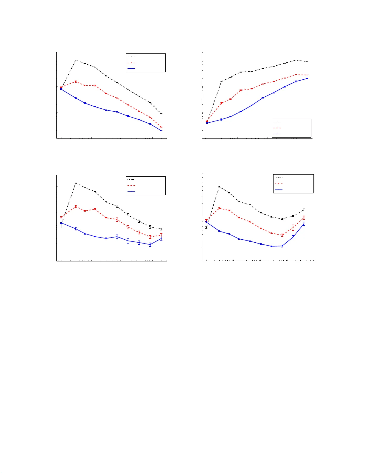
A Randomized Nonmonoto ne Blo c k Pro ximal Gradien t Metho d for a Class of Structure d Nonlinear Programming Zhaoson g Lu ∗ Lin Xiao † July 30, 2018 Abstract W e prop ose a randomized nonmonotone b lo c k proxima l gradient (RNBPG) metho d for minimizing the su m of a smo oth (p ossibly noncon v ex) function and a b lo c k-separable (p ossibly noncon vex non s mo oth) function. A t eac h iteration, this metho d randomly pic ks a blo c k according to an y prescrib ed probabilit y distribution and solv es t yp ically sev eral asso ciated pro ximal su bproblems that usually ha ve a closed-form solution, un til a certain progress on ob jectiv e v alue is ac hiev ed. In con trast to the us ual randomized blo c k co ordinate descen t metho d [23, 20], our metho d h as a non m onotone flav or and uses v ariable stepsizes that can p artially utilize the lo cal curv ature in f ormation of the smo oth comp onent of ob jectiv e function. W e sho w that an y acc u m ulation p oint of th e solution sequence of th e metho d is a stationary p oin t of the problem almost sur ely and the metho d is capable of fi nding an approxi mate stationary p oin t with high probabil- it y . W e also establish a sublinear rate of con verge n ce for the metho d in terms of the minimal exp ected squared norm of certain pro ximal gradients ov er the iterations. When the problem u nder consideration is con ve x, w e show that the exp ected ob jectiv e v al- ues generated by RNBPG con verge to the optimal v alue of the p r oblem. Under some assumptions, we further establish a s u blinear and linear rate of con v ergence on the ex- p ected ob jectiv e v alues generated b y a monotone version of RNBPG. Finally , we conduct some preliminary exp erimen ts to test the p erform an ce of RNBPG on th e ℓ 1 -regularized least-squares p roblem and a dual SVM problem in m achine learning. The computa- tional results demonstrate that our metho d sub stan tially outp erforms th e randomized blo c k co ordinate desc ent metho d with fixed or v ariable stepsizes. Key words: nonconv ex comp osite optimization, rand omized algorithms, blo c k coordi- nate gradient metho d, n onmonotone line searc h. ∗ Department of Mathematics, Simon F ras er University , Burnab y , BC, V5A 1S6, Canada . (email: zhaoso ng@sf u.ca ). This author was s uppo rted in pa rt by NSER C Discovery Gra nt. † Machine Lea rning Groups, Micr osoft Resear ch, One Mic r osoft W ay , Redmond, W A 98052 , USA. (email: lin.xi ao@mi crosoft .com ). 1 1 In tro duction No w adays first-order (namely , gradient-t yp e) metho ds are the prev alent to ols for solving large- scale problems arising in science and engineering. As the size of problems b ecomes h uge, it is, ho w ev er, greatly challenging to these metho ds b ecause gradien t ev aluation can b e prohibitiv ely exp ensiv e. Due to this reason, blo c k co ordinate descen t (BCD) metho ds and t heir v ariants ha v e been studied fo r solving v a rious large-scale pro blems (see, for example, [4, 12, 3 6, 14 , 30, 31, 3 3 , 34, 21, 37, 25, 1 3, 22, 26, 24, 28]). Recen tly , Nestero v [1 8] pro p osed a randomized BCD (RBCD) metho d, whic h is promising for solving a class of h uge-scale conv ex optimization problems, pro vided the in volv ed partial gradien ts can b e efficien tly up dated. The iteration complexit y for finding a n approximate optimal solution is analyzed in [18]. More recen tly , Ric h t´ arik and T ak´ a ˇ c [23] extended Nestero v’s RBCD metho d [18] to solv e a more general class of con vex optimization problems in the form of min x ∈ℜ N { F ( x ) := f ( x ) + Ψ( x ) } , (1) where f is conv ex differentiable in ℜ N and Ψ is a block separable conv ex function. More sp ecifically , Ψ( x ) = n X i =1 Ψ i ( x i ) , where eac h x i denotes a sub v ector of x with cardinality N i , { x i : i = 1 , . . . , n } form a partition of the comp onen ts o f x , and eac h Ψ i : ℜ N i → ℜ ∪ { + ∞} is a closed con vex function. Giv en a current iterate x k , the RBCD metho d [23] pic ks i ∈ { 1 , . . . , n } uniformly , solves a blo c k-wise pro ximal subproblem in the form of d i ( x k ) := arg min s ∈ℜ N i  ∇ i f ( x k ) T s + L i 2 k s k 2 + Ψ i ( x k i + s )  , (2) and sets x k +1 i = x k i + d i ( x k ) a nd x k +1 j = x k j for all j 6 = i , where ∇ i f ∈ ℜ N i is the p artial gr adient of f with resp ect to x i and L i > 0 is the Lipsc hitz constan t of ∇ i f with resp ect to the norm k · k (see Assumption 1 for details). The iteration complexit y of finding an approx imate optimal solution with high pro babilit y is established in [23 ] and has recen tly b een impro v ed by Lu and Xiao [15]. V ery recen tly , P atrascu and Necoara [2 0] extended this metho d to solv e problem (1) in whic h F is noncon vex , and they studied con ve rg ence o f the metho d under the assumption that the blo c k is c hosen uniformly at each iteration. One can o bserv e tha t for n = 1, the RBCD method [23, 20] b ecomes a classical pro ximal (full) gradien t metho d with a constan t stepsize 1 /L . It is kno wn tha t t he lat t er metho d tends to b e practically muc h slo w er than the same type of metho ds but with v ariable stepsizes, for example, spectral-type stepsize [1, 3, 6, 35, 16]) that utilizes partial lo cal curv at ure infor- mation of the smo oth comp onen t f . The v ariable stepsize strategy shall also b e applicable to the RBCD metho d a nd improv e its pr a ctical p erformance dramatically . In addition, the RBCD metho d is a monotone metho d, that is, the ob jectiv e v alues generated b y the metho d 2 are monotonically dec reasing. As mentioned in the lit erature (see, for example, [8, 9, 38 ]), nonmonotone metho ds often pro duce solutions of b etter quality than the monot o ne coun- terparts fo r nonconv ex optimization problems. These motiv ate us to prop ose a rando mized nonmonotone blo c k pro ximal gradien t metho d with v ariable stepsiz es for solving a class of (p ossibly noncon vex ) structured nonlinear progr a mming problems in the form of (1) satisfy- ing Assumption 1 b elo w. Throughout this pap er w e assume that the set of optimal solutions of problem (1), de- noted b y X ∗ , is nonempt y and the optimal v a lue of (1) is denoted by F ⋆ . F or simplicit y of presen ta tion, w e asso ciate ℜ N with the standard Euclidean norm, denoted b y k · k . W e also mak e the follow ing assumption. Assumption 1 f is differ entiable (but p ossibly nonc onvex ) in ℜ N . Each Ψ i is a (p ossibly nonc on vex nonsmo oth) function fr om ℜ N i to ℜ ∪ { + ∞} for i = 1 , . . . , n . The gr adient of function f i s c o or dina te-wise Lip schitz c ontinuous with c onstants L i > 0 in ℜ N , that is, k∇ i f ( x + h ) − ∇ i f ( x ) k ≤ L i k h k ∀ h ∈ S i , i = 1 , . . . , n, ∀ x ∈ ℜ N , wher e S i =  ( h 1 , . . . , h n ) ∈ ℜ N 1 × · · · × ℜ N n : h j = 0 ∀ j 6 = i  . In this pap er w e prop ose a randomized nonmonotone blo c k pro ximal g radien t ( RNBPG) metho d fo r solving problem (1) t hat satisfies the a b ov e assumptions. A t each iteration, this metho d ra ndomly pic ks a blo c k according to an arbitra r y prescrib ed (not necessarily uniform) probabilit y distribution and solv es t ypically sev eral asso ciated proximal subproblems in the form of (2) with L i replaced b y some θ , which can b e, for example, estimated b y the sp ectral metho d (e.g., see [1, 3 , 6, 35, 16]), un til a certain prog r ess on the ob jectiv e v a lue is a c hiev ed. In con trast to the usual RBCD metho d [23 , 20], our method enjo ys a no nmono t one fla vor and use s v ariable stepsize s tha t can partially utilize the lo cal curv ature information of the smo oth comp onen t f . F or arbitrary probabilit y distribution 1 , W e sho w that the exp ected ob jectiv e v alues generated by the metho d con v erge to t he exp ected limit of the ob jectiv e v alues obtained b y a random single run of the metho d. Moreo v er, any accum ula t ion p oin t of the solution sequence of the metho d is a stationary p o int of the problem almost sur ely and the metho d is capable of finding an appro ximate stationa r y p oin t with high probabilit y . W e also establish a sublinear rate of con ve rgence fo r t he metho d in terms of t he minimal exp ected squared norm of certain prox imal gradien ts o v er the iterations. When the problem under consideration is con v ex, w e sho w that the expected ob jectiv e v alues g enerated by RNBPG con v erge to the optimal v alue of the problem. Under some assumptions, we further establish a sublinear and linear rate of conv ergence on the exp ected ob jectiv e v alues generated b y a monotone v ersion of RNBPG. Finally , w e conduct some preliminary exp erimen ts to test the p erformance of R NBPG on the ℓ 1 -regularized least-squares pro blem and a dual SVM problem 1 The conv erg ence a nalysis o f the RBCD metho d conducted in [2 3, 20] is o nly for uniform proba bility distribution. 3 in machine learning. The computational results demonstrate that our metho d substantially outp erforms the rando mized blo c k co ordinate desc ent metho d with fixed or v aria ble stepsizes. This pap er is organized as follo ws. In Section 2 w e prop ose a RNBPG method for solving structured nonlinear prog ramming problem (1) and analyze its con v ergence. In Section 3 w e analyze the conv ergence of RNBPG for solving structured con v ex problem. In Section 4 w e conduct numerical exp erimen ts to compare RNBPG me tho d with the RBCD method with fixed or v a r iable stepsizes. Before ending this section w e in tro duce some nota tions t ha t are used throughout this pap er and also state some kno wn facts. The do ma in of the function F is denoted b y do m( F ). t + stands for max { 0 , t } for any real n umber t . Giv en a close d set S and a p oint x , dist( x, S ) denotes the distance b et w een x and S . F or symmetric matrices X and Y , X  Y means that Y − X is p ositiv e semidefinite. Giv en a p ositive definite matrix Θ and a v ector x , k x k Θ = √ x T Θ x . In addition, k · k denotes the Euclidean norm. Finally , it immediately follo ws from Assumption 1 that f ( x + h ) ≤ f ( x ) + ∇ f ( x ) T h + L i 2 k h k 2 ∀ h ∈ S i , i = 1 , . . . , n ; ∀ x ∈ ℜ N . (3) By Lemma 2 of Nestero v [18] a nd Assumption 1, w e also kno w that ∇ f is Lipsc hitz contin uous with constan t L f := P i L i , that is, k∇ f ( x ) − ∇ f ( y ) k ≤ L f k x − y k x, y ∈ ℜ N . (4) 2 Randomized non monotone blo c k pro ximal g radien t metho d In this section w e prop ose a RNBPG metho d for solving structured nonlinear progr amming problem (1) and analyze its con v ergence. W e start by presen ting a RNBPG metho d as follo ws. A t eac h iteration, this metho d randomly picks a blo c k according to an y prescribed (not neces sarily uniform) probabilit y distribution and solve s typic ally sev eral asso ciated proximal subproblems in the fo rm of (2) with L i replaced by some θ k un til a certain progress on ob jectiv e v alue is ac hiev ed. Randomized nonmonotone blo ck proxim al gradien t ( RNBPG) metho d Cho ose x 0 ∈ dom( F ), η > 1, σ > 0, 0 < θ ≤ ¯ θ , in teger M ≥ 0 , a nd 0 < p i < 1 for i = 1 , . . . , n suc h that P n i =1 p i = 1. Set k = 0. 1) Set d k = 0. Pic k i k = i ∈ { 1 , . . . , n } with probabilit y p i . Cho ose θ 0 k ∈ [ θ , ¯ θ ]. 2) F or j = 0 , 1 , . . . 2a) Let θ k = θ 0 k η j . Compute ( d k ) i k = arg min s  ∇ i k f ( x k ) T s + θ k 2 k s k 2 + Ψ i k ( x k i k + s )  . (5) 4 2b) If d k satisfies F ( x k + d k ) ≤ max [ k − M ] + ≤ i ≤ k F ( x i ) − σ 2 k d k k 2 , (6) go to step 3). 3) Set x k +1 = x k + d k , k ← k + 1 and go to step 1). end Remark 2.1 The ab ove metho d b e c omes a monotone metho d if M = 0 . Before studying conv ergence of RNBPG, w e introduce some notations and state some facts that will b e used subsequen tly . Let ¯ d k ,i denote the v ector d k obtained in Step (2) of R NBPG if i k is chose n to b e i . Define ¯ d k = n X i =1 ¯ d k ,i , ¯ x k = x k + ¯ d k . (7) One can o bserv e that ( ¯ d k ,i ) t = 0 for t 6 = i and there exist θ 0 k ,i ∈ [ θ , ¯ θ ] and the smallest nonnegativ e in teger j suc h that θ k ,i = θ 0 k ,i η j and F ( x k + ¯ d k ,i ) ≤ F ( x ℓ ( k ) ) − σ 2 k ¯ d k ,i k 2 , (8) where ( ¯ d k ,i ) i = arg min s  ∇ i f ( x k ) T s + θ k ,i 2 k s k 2 + Ψ i ( x k i + s )  , (9) ℓ ( k ) = arg max i { F ( x i ) : i = [ k − M ] + , . . . , k } ∀ k ≥ 0 . (10) Let Θ k denote the blo c k diagonal matrix ( θ k , 1 I 1 , . . . , θ k ,n I n ), where I i is the N i × N i iden tit y matrix. By the definition of ¯ d k and (9), w e observ e that ¯ d k = arg min d  ∇ f ( x k ) T d + 1 2 d T Θ k d + Ψ( x k + d )  . (11) After k iterations, RNBPG generates a random o utput ( x k , F ( x k )), whic h dep ends on the observ ed realization of random v ector ξ k = { i 0 , . . . , i k } . W e define E ξ − 1 [ F ( x 0 )] = F ( x 0 ). Also, define Ω( x 0 ) = { x ∈ ℜ N : F ( x ) ≤ F ( x 0 ) } , (12) L max = max i L i , p min = min i p i , (13) c = max  ¯ θ , η ( L max + σ )  . (14) The following lemma establishes some r elat io ns b et wee n the exp ectatio ns of k d k k and k ¯ d k k . 5 Lemma 2.2 L et d k b e gener ate d by RNBPG and ¯ d k define d in (7). Ther e hold E ξ k [ k d k k 2 ] ≥ p min E ξ k − 1 [ k ¯ d k k 2 ] , (15) E ξ k [ k d k k ] ≥ p min E ξ k − 1 [ k ¯ d k k ] . (16) Pr o of . By (1 3) and the definitions of d k and ¯ d k , we can observ e that E i k [ k d k k 2 ] = P i p i k ¯ d k ,i k 2 ≥ (min i p i ) P i k ¯ d k ,i k 2 = p min k ¯ d k k 2 , E i k [ k d k k ] = P i p i k ¯ d k ,i k ≥ (min i p i ) P i k ¯ d k ,i k ≥ p min r P i k ¯ d k ,i k 2 ≥ p min k ¯ d k k . The conclusion of this lemma follow s by taking exp ectatio n with r esp ect to ξ k − 1 on b o th sides of the a b ov e inequalities. W e next show that the inner lo ops of the ab ov e R NBPG metho d m ust terminate finitely . As a byp ro duct, we pro vide a uniform upper b ound on Θ k . Lemma 2.3 L et { θ k } b e the s e quenc e g ener ate d b y RNBPG, Θ k define d ab ove, and c defin e d in (14). T h er e hold (i) θ ≤ θ k ≤ c ∀ k . (ii) θ I  Θ k  cI ∀ k . Pr o of . (i) It is clear tha t θ k ≥ θ . W e no w sho w θ k ≤ c by dividing the pro o f into t w o cases. Case (i) θ k = θ 0 k . Since θ 0 k ≤ ¯ θ , it follo ws that θ k ≤ ¯ θ and the conclus ion holds. Case (ii) θ k = θ 0 k η j for some in teger j > 0. Supp ose for con tradiction that θ k > c . By (13) and (14), w e then hav e ˜ θ k := θ k /η > c/η ≥ L max + σ ≥ L i k + σ . (17) Let d ∈ ℜ N suc h that d i = 0 f o r i 6 = i k and d i k = arg min s ( ∇ i k f ( x k ) T s + ˜ θ k 2 k s k 2 + Ψ i k ( x k i k + s ) ) . (18) It follows that ∇ i k f ( x k ) T d i k + ˜ θ k 2 k d i k k 2 + Ψ i k ( x k i k + d i k ) − Ψ i k ( x k i k ) ≤ 0 . Also, by (10) and the definitions of θ k and ˜ θ k , one knows that F ( x k + d ) > F ( x ℓ ( k ) ) − σ 2 k d k 2 . (19) 6 On the other hand, using (3), (10), (1 7), (18) and the definition of d , w e ha v e F ( x k + d ) = f ( x k + d ) + Ψ( x k + d ) ≤ f ( x k ) + ∇ i k f ( x k ) T d i k + L i k 2 k d i k k 2 + Ψ( x k + d ) = F ( x k ) + ∇ i k f ( x k ) T d i k + ˜ θ k 2 k d i k k 2 + Ψ i k ( x k i k + d i k ) − Ψ i k ( x k i k ) | {z } ≤ 0 + L i k − ˜ θ k 2 k d i k k 2 ≤ F ( x k ) + L i k − ˜ θ k 2 k d i k k 2 ≤ F ( x ℓ ( k ) ) − σ 2 k d k 2 , whic h is a con tradiction to (19 ). Hence, θ k ≤ c and the conclusion holds. (ii) Let θ k ,i b e defined ab ov e. It follo ws from statemen t (i) that θ ≤ θ k ,i ≤ c , whic h together with the definition of Θ k implies that statemen t (ii) holds. The next result provides some b ound on the no rm of a proximal gradien t, whic h will b e used in the subsequen t analysis on con vergenc e rate o f RNBPG. Lemma 2.4 L et { x k } b e gener a te d by RNBPG, ¯ d k and c defin e d in (11) and (14), r e sp e ctively, and ˆ g k = arg min d  ∇ f ( x k ) T d + 1 2 k d k 2 + Ψ( x k + d )  . (20) Assume that Ψ is c onvex. Ther e holds k ˆ g k k ≤ c 2 " 1 + 1 θ + s 1 − 2 c + 1 θ 2 # k ¯ d k k . (21) Pr o of . The conclusion of this lemma follo ws from (11), (20), Lemma 2.3 (ii), and [16, Lemma 3.5] with H = Θ k , ˜ H = I , Q = Θ − 1 k , d = ¯ d k and ˜ d = ˆ g k . W e note that b y the definition in (14), w e ha v e c ≥ θ > θ , whic h implies 1 − 2 c + 1 θ 2 =  1 − 1 θ  2 + 2 θ − 2 c > 0 . Therefore, the expres sion under the square ro ot in (21) is alw a ys p ositiv e. 2.1 Con ve rgence of exp ected ob jectiv e v alue In this subsection w e sho w tha t the sequence o f exp ected ob jectiv e v a lues g enerated b y the metho d con v erge to the exp ected limit of t he ob jectiv e v a lues obtained b y a r andom single run of the metho d. The following lemma studies uniform con tin uity of the exp ectation of F with resp ect to random sequences. 7 Lemma 2.5 Supp ose that F is uniform c ontinuous in some S ⊆ dom ( F ) . L et y k and z k b e two r andom ve ctors in S g e ner ate d fr om ξ k − 1 . Assume that ther e e xists C > 0 s uch that | F ( y k ) − F ( z k ) | ≤ C for al l k , and mor e over, lim k →∞ E ξ k − 1 [ k y k − z k k ] = 0 . Then ther e hold lim k →∞ E ξ k − 1 [ | F ( y k ) − F ( z k ) | ] = 0 , lim k →∞ E ξ k − 1 [ F ( y k ) − F ( z k )] = 0 . Pr o of . Since F is uniformly con tinuous in S , it fo llo ws that giv en an y ǫ > 0, there exists δ ǫ > 0 suc h that | F ( x ) − F ( y ) | < ǫ/ 2 for all x, y ∈ S satisfying k x − y k < δ ǫ . Using these relations, the Mark ov inequality , and the assumption that | F ( y k ) − F ( z k ) | ≤ C for all k and lim k →∞ E ξ k − 1 [ k ∆ k k ] = 0, where ∆ k = y k − z k , w e obtain that for sufficien tly large k , E ξ k − 1 [ | F ( y k ) − F ( z k ) | ] = E ξ k − 1  | F ( y k ) − F ( z k ) |   k ∆ k k ≥ δ ǫ  P ( k ∆ k k ≥ δ ǫ ) + E ξ k − 1  | F ( y k ) − F ( z k ) |   k ∆ k k < δ ǫ  P ( k ∆ k k < δ ǫ ) ≤ C E ξ k − 1 [ k ∆ k k ] δ ǫ + ǫ 2 ≤ ǫ. Due to the arbitra r ily of ǫ , w e see that the first statemen t of this lemma holds. The second statemen t immediately follows from the first statemen t and the w ell-kno wn inequalit y | E ξ k − 1 [ F ( y k ) − F ( z k )] | ≤ E ξ k − 1  | F ( y k ) − F ( z k ) |  . W e are ready t o establish the first main result, that is, the expected ob j ective v alues generated by the RNBPG metho d con v erge to the expected limit of the ob jectiv e v alues obtained by a random single run of the metho d. Theorem 2.6 L et { x k } and { d k } b e the se quenc es ge ner ate d by the RNB PG metho d. Assume that F is uniform c on tinuous in Ω( x 0 ) , wher e Ω( x 0 ) is define d in (1 2). Then the fol low i n g statements hold: (i) lim k →∞ [ k d k k ] = 0 and lim k →∞ F ( x k ) = F ∗ ξ ∞ for som e F ∗ ξ ∞ ∈ ℜ , wher e ξ ∞ = { i 1 , i 2 , · · · } . (ii) lim k →∞ E ξ k [ k d k k ] = 0 a n d lim k →∞ E ξ k − 1 [ F ( x k )] = lim k →∞ E ξ k − 1 [ F ( x ℓ ( k ) )] = E ξ ∞ [ F ∗ ξ ∞ ] . (22) Pr o of . By (6) and (10), w e ha ve F ( x k +1 ) ≤ F ( x ℓ ( k ) ) − σ 2 k d k k 2 ∀ k ≥ 0 . (23) 8 Hence, F ( x k +1 ) ≤ F ( x ℓ ( k ) ), whic h together with (10) implies t hat F ( x ℓ ( k + 1) ) ≤ F ( x ℓ ( k ) ). It then follows that E ξ k [ F ( x ℓ ( k + 1) )] ≤ E ξ k − 1 [ F ( x ℓ ( k ) )] ∀ k ≥ 1 . Hence, { F ( x ℓ ( k ) ) } and { E ξ k − 1 [ F ( x ℓ ( k ) )] } are non-increasing. Since F is b ounded b elo w, so are { F ( x ℓ ( k ) ) } and { E ξ k − 1 [ F ( x ℓ ( k ) )] } . It follows that there exis t some F ∗ ξ ∞ , ˜ F ∗ ∈ ℜ suc h that lim k →∞ F ( x ℓ ( k ) ) = F ∗ ξ ∞ , lim k →∞ E ξ k − 1 [ F ( x ℓ ( k ) )] = ˜ F ∗ . ( 2 4) W e first sho w b y induction that the follo wing relations hold fo r all j ≥ 1: lim k →∞ k d ℓ ( k ) − j k = 0 , lim k →∞ F ( x ℓ ( k ) − j ) = F ∗ ξ ∞ . (25) lim k →∞ E ξ k − 1 [ k d ℓ ( k ) − j k ] = 0 , lim k →∞ E ξ k − 1 [ F ( x ℓ ( k ) − j )] = ˜ F ∗ . (26) Indeed, replacing k b y ℓ ( k ) − 1 in (23), w e obtain that F ( x ℓ ( k ) ) ≤ F ( x ℓ ( ℓ ( k ) − 1) ) − σ 2 k d ℓ ( k ) − 1 k 2 ∀ k ≥ M + 1 , whic h together with ℓ ( k ) ≥ k − M and monot o nicit y of { F ( x ℓ ( k ) ) } yields F ( x ℓ ( k ) ) ≤ F ( x ℓ ( k − M − 1) ) − σ 2 k d ℓ ( k ) − 1 k 2 ∀ k ≥ M + 1 . (27) Then we hav e E ξ k − 1 [ F ( x ℓ ( k ) )] ≤ E ξ k − 1 [ F ( x ℓ ( k − M − 1) )] − σ 2 E ξ k − 1 [ k d ℓ ( k ) − 1 k 2 ] ∀ k ≥ M + 1 . (28) Notice that E ξ k − 1 [ F ( x ℓ ( k − M − 1) )] = E ξ k − M − 2 [ F ( x ℓ ( k − M − 1) )] ∀ k ≥ M + 1 . It follows from this relation and (28) that E ξ k − 1 [ F ( x ℓ ( k ) )] ≤ E ξ k − M − 2 [ F ( x ℓ ( k − M − 1) )] − σ 2 E ξ k − 1 [ k d ℓ ( k ) − 1 k 2 ] ∀ k ≥ M + 1 . (29) In view of (24), (27), (29), and ( E ξ k − 1 [ k d ℓ ( k ) − 1 k ]) 2 ≤ E ξ k − 1 [ k d ℓ ( k ) − 1 k 2 ], one can ha v e lim k →∞ k d ℓ ( k ) − 1 k = 0 , lim k →∞ E ξ k − 1 [ k d ℓ ( k ) − 1 k ] = 0 . (30) One can also o bserv e that F ( x k ) ≤ F ( x 0 ) and hence { x k } ⊂ Ω( x 0 ). Using this f a ct, ( 24), (30), Lemma 2.5, a nd uniform con tin uity of F ov er Ω( x 0 ), w e obtain that lim k →∞ F ( x ℓ ( k ) − 1 ) = lim k →∞ F ( x ℓ ( k ) ) = F ∗ ξ ∞ , lim k →∞ E ξ k − 1 [ F ( x ℓ ( k ) − 1 )] = lim k →∞ E ξ k − 1 [ F ( x ℓ ( k ) )] = ˜ F ∗ . 9 Therefore, (25) and ( 26) hold for j = 1 . Suppose now that they hold for some j ≥ 1. W e need to sho w that they also hold for j + 1. Replacing k b y ℓ ( k ) − j − 1 in (23) giv es F ( x ℓ ( k ) − j ) ≤ F ( x ℓ ( ℓ ( k ) − j − 1) ) − σ 2 k d ℓ ( k ) − j − 1 k 2 ∀ k ≥ M + j + 1 . By this relat io n, ℓ ( k ) ≥ k − M , and monotonicit y of { F ( x ℓ ( k ) ) } , one can ha v e F ( x ℓ ( k ) − j ) ≤ F ( x ℓ ( k − M − j − 1) ) − σ 2 k d ℓ ( k ) − j − 1 k 2 ∀ k ≥ M + j + 1 . (31) Then we obta in that E ξ k − 1 [ F ( x ℓ ( k ) − j )] ≤ E ξ k − 1 [ F ( x ℓ ( k − M − j − 1) )] − σ 2 k d ℓ ( k ) − j − 1 k 2 ∀ k ≥ M + j + 1 . Notice that E ξ k − 1 [ F ( x ℓ ( k − M − j − 1) )] = E ξ k − M − j − 2 [ F ( x ℓ ( k − M − j − 1) )] ∀ k ≥ M + j + 1 . It follows from these tw o relations that E ξ k − 1 [ F ( x ℓ ( k ) − j )] ≤ E ξ k − M − j − 2 [ F ( x ℓ ( k − M − j − 1) )] − σ 2 E ξ k − 1 [ k d ℓ ( k ) − j − 1 k 2 ] , ∀ k ≥ M + j + 1 . (32) Using ( 24), (31), ( 3 2), the induction h yp o thesis, and a s imilar argumen t as ab o v e, w e can obtain that lim k →∞ k d ℓ ( k ) − j − 1 k = 0 , lim k →∞ E ξ k − 1 [ k d ℓ ( k ) − j − 1 k ] = 0 . These relations, together with Lemma 2.5, uniform contin uity of F ov er Ω( x 0 ) and the induc- tion hypothesis, yield lim k →∞ F ( x ℓ ( k ) − j − 1 ) = lim k →∞ F ( x ℓ ( k ) − j ) = F ∗ ξ ∞ , lim k →∞ E ξ k − 1 [ F ( x ℓ ( k ) − j − 1 )] = lim k →∞ E ξ k − 1 [ F ( x ℓ ( k ) − j )] = ˜ F ∗ . Hence, (25) and (26) hold for j + 1, and the pro of of (25) and (26) is completed. F or all k ≥ 2 M + 1, we define ˜ d ℓ ( k ) − j =  d ℓ ( k ) − j if j ≤ ℓ ( k ) − ( k − M − 1) , 0 otherwise , j = 1 , . . . , M + 1 . It is not hard to o bserv e that k ˜ d ℓ ( k ) − j k ≤ k d ℓ ( k ) − j k , (33) x ℓ ( k ) = x k − M − 1 + M + 1 X j =1 ˜ d ℓ ( k ) − j . (34) 10 It follow s fro m (2 5 ), (2 6) and (33) that lim k →∞ k ˜ d ℓ ( k ) − j k = 0 and lim k →∞ E ξ k − 1 [ k ˜ d ℓ ( k ) − j k ] = 0 for j = 1 , . . . , M + 1. Hence, lim k →∞      M + 1 X j =1 ˜ d ℓ ( k ) − j      = 0 , lim k →∞ E ξ k − 1 "      M + 1 X j =1 ˜ d ℓ ( k ) − j      # = 0 . These, together with (25), (26), (34), Lemma 2.5 and uniform con tin uity of F ov er Ω( x 0 ), imply that lim k →∞ F ( x k − M − 1 ) = lim k →∞ F ( x ℓ ( k ) ) = F ∗ ξ ∞ , (35) lim k →∞ E ξ k − 1 [ F ( x k − M − 1 )] = lim k →∞ E ξ k − 1 [ F ( x ℓ ( k ) )] = ˜ F ∗ . (36) It follow s from (35) that lim k →∞ F ( x k ) = F ∗ ξ ∞ . Using this, (23) and (24), one can see that lim k →∞ k d k k = 0. Henc e, stat ement (i) ho lds. Notice that E ξ k − M − 2 [ F ( x k − M − 1 )] = E ξ k − 1 [ F ( x k − M − 1 )]. Com bining this relation with (36), w e ha ve lim k →∞ E ξ k − M − 2 [ F ( x k − M − 1 )] = ˜ F ∗ , whic h is equiv a len t to lim k →∞ E ξ k − 1 [ F ( x k )] = ˜ F ∗ . In addition, it follo ws from (23) t ha t E ξ k [ F ( x k +1 )] ≤ E ξ k [ F ( x ℓ ( k ) )] − σ 2 E ξ k [ k d k k 2 ] ∀ k ≥ 0 . (37) Notice that lim k →∞ E ξ k [ F ( x ℓ ( k ) )] = lim k →∞ E ξ k − 1 [ F ( x ℓ ( k ) )] = ˜ F ∗ = lim k →∞ E ξ k [ F ( x k +1 )] . (38) Using (37) and (38), we conclude that lim k →∞ E ξ k [ k d k k ] = 0. Finally , w e claim that lim k →∞ E ξ k − 1 [ F ( x k )] = E ξ ∞ [ F ∗ ξ ∞ ]. Inde ed, we kno w that { x k } ⊂ Ω( x 0 ). Hence, F ∗ ≤ F ( x k ) ≤ F ( x 0 ), where F ∗ = min x F ( x ). It follows that | F ( x k ) | ≤ max { | F ( x 0 ) | , | F ∗ |} ∀ k . Using this relation and dominat ed con ve rgence theorem (see, for example, [2, Theorem 5.4]), w e ha v e lim k →∞ E ξ ∞ [ F ( x k )] = E ξ ∞ h lim k →∞ F ( x k ) i = E ξ ∞  F ∗ ξ ∞  , whic h, to g ether with lim k →∞ E ξ k − 1 [ F ( x k )] = lim k →∞ E ξ ∞ [ F ( x k )], implies that lim k →∞ E ξ k − 1 [ F ( x k )] = E ξ ∞ [ F ∗ ξ ∞ ]. Hence, statement (ii) holds. 11 2.2 Con ve rgence to stationary p oin ts In this subsec tion w e sho w that when k is sufficien tly large, x k is an appro ximate stationary p oint o f (1) with high probability . Theorem 2.7 L et { x k } b e gener ate d by RNBPG, and ¯ d k and ¯ x k define d in (7). Assume that F is uniformly c ontinuous and Ψ is lo c al ly Lipschitz c ontinuous in Ω( x 0 ) , wher e Ω( x 0 ) is define d in (12). Then ther e hold (i) lim k →∞ E ξ k − 1 [ k ¯ d k k ] = 0 , lim k →∞ E ξ k − 1 [dist( −∇ f ( ¯ x k ) , ∂ Ψ( ¯ x k )] = 0 , (3 9) wher e ∂ Ψ deno tes the Clarke sub d iffer ential of Ψ . (ii) A ny ac cumulation p oint of { x k } is a stationary p oint of pr ob l e m (1) almost sur ely. (iii) Supp ose further that F is uniformly c ontinuous in S = n x : F ( x ) ≤ F ( x 0 ) + max n n σ | L f − θ | , 1 o ( F ( x 0 ) − F ∗ ) o . (40) Then lim k →∞ E ξ k − 1 [ | F ( x k ) − F ( ¯ x k ) | ] = 0 . Mor e over, for any ǫ > 0 and ρ ∈ (0 , 1) , ther e exists K such that for al l k ≥ K , P  max  k x k − ¯ x k k , | F ( x k ) − F ( ¯ x k ) | , dist( −∇ f ( ¯ x k ) , ∂ Ψ( ¯ x k ))  ≤ ǫ  ≥ 1 − ρ. Pr o of . (i) W e kno w from Theorem 2 .6 (ii) that lim k →∞ E ξ k [ k d k k ] = 0, whic h together with (16) implies lim k →∞ E ξ k − 1 [ k ¯ d k k ] = 0. Notice that ¯ d k is an optimal solution of problem (1 1). By the first-order optimality condition (see, for example, Prop osition 2.3.2 of [5]) of (11) and ¯ x k = x k + ¯ d k , one can ha v e 0 ∈ ∇ f ( x k ) + Θ k ¯ d k + ∂ Ψ( ¯ x k ) . (41) In addition, it follo ws from (4) that k∇ f ( ¯ x k ) − ∇ f ( x k ) k ≤ L f k ¯ d k k . Using this relat io n along with Lemma 2.3 (ii) and ( 4 1), w e obtain that dist( −∇ f ( ¯ x k ) , ∂ Ψ( ¯ x k )) ≤ ( c + L f ) k ¯ d k k , whic h together with the first relation of ( 39) implies that the second relation of ( 3 9) also holds. (ii) Let x ∗ b e an accumulation p oin t of { x k } . T here exists a subsequence K suc h that lim k ∈K→∞ x k = x ∗ . Since E ξ k − 1 [ k ¯ d k k ] → 0, it follo ws that { ¯ d k } k ∈K → 0 almost surely . This together with the second relatio n of (39) and out er semi-con tin uity of ∂ Ψ yields dist( −∇ f ( x ∗ ) , ∂ Ψ( x ∗ )) = lim k ∈K→∞ dist( −∇ f ( ¯ x k ) , ∂ Ψ( ¯ x k )) = 0 12 almost surely . Hence, x ∗ is a stationary p oin t of problem (1) almost surely . (iii) Recall that ¯ x k = x k + ¯ d k . It follows from (4) t ha t f ( ¯ x k ) ≤ f ( x k ) + ∇ f ( x k ) T ¯ d k + 1 2 L f k ¯ d k k 2 . Using this relat io n and Lemma 2.3 (ii), w e hav e F ( ¯ x k ) ≤ f ( x k ) + ∇ f ( x k ) T ¯ d k + 1 2 L f k ¯ d k k 2 + Ψ( x k + ¯ d k ) ≤ f ( x k ) + ∇ f ( x k ) T ¯ d k + 1 2 ( ¯ d k ) T Θ k ¯ d k + Ψ( x k + ¯ d k ) + 1 2 ( L f − θ ) k ¯ d k k 2 . (42) In view of (11), one has ∇ f ( x k ) T ¯ d k + 1 2 ( ¯ d k ) T Θ k ¯ d k + Ψ( x k + ¯ d k ) ≤ Ψ ( x k ) , whic h together with (42 ) yields F ( ¯ x k ) ≤ F ( x k ) + 1 2 ( L f − θ ) k ¯ d k k 2 . Using this relat io n and the fact that F ( ¯ x k ) ≥ F ∗ and F ( x k ) ≤ F ( x 0 ), one can obtain that | F ( ¯ x k ) − F ( x k ) | ≤ max  1 2 | L f − θ | k ¯ d k k 2 , F ( x 0 ) − F ∗  ∀ k . (43) In additio n, since F l ( k ) ≤ F ( x 0 ) and F ( ¯ x k ) ≥ F ∗ , it follow s f rom (8) that k ¯ d k ,i k 2 ≤ 2( F ( x 0 ) − F ∗ ) /σ . Hence, one has k ¯ d k k 2 = n X i =1 k ¯ d k ,i k 2 ≤ 2 n ( F ( x 0 ) − F ∗ ) /σ ∀ k . This inequalit y together with (43) yields | F ( ¯ x k ) − F ( x k ) | ≤ max n n σ | L f − θ | , 1 o ( F ( x 0 ) − F ∗ ) ∀ k , and hence {| F ( ¯ x k ) − F ( x k ) |} is b ounded. Also, this inequality t o gether with F ( x k ) ≤ F ( x 0 ) and the definition of S implies that ¯ x k , x k ∈ S for a ll k . In a ddition, b y statemen t (i), we kno w E ξ k − 1 [ k x k − ¯ x k k ] → 0 . In view of these facts and inv oking Lemma 2 .5, one has lim k →∞ E ξ k − 1 [ | F ( x k ) − F ( ¯ x k ) | ] = 0 . (44) Observ e that 0 ≤ max  k x k − ¯ x k k , | F ( x k ) − F ( ¯ x k ) | , dist( −∇ f ( ¯ x k ) , ∂ Ψ( ¯ x k ))  ≤ k x k − ¯ x k k + | F ( x k ) − F ( ¯ x k ) | + dist( −∇ f ( ¯ x k ) , ∂ Ψ( ¯ x k )) . Using these inequalities , (44) and statemen t (i), w e see that lim k →∞ E ξ k − 1  max  k x k − ¯ x k k , | F ( x k ) − F ( ¯ x k ) | , dist( −∇ f ( ¯ x k ) , ∂ Ψ( ¯ x k ))  = 0 . The rest of statemen t (iii) follows fro m this relation and the Mark ov inequalit y . 13 2.3 Con ve rgence rate analysis In this subs ection we establis h a sublinear rate of con ve rgence of RNBPG in terms of the minimal exp ected squared norm of certain proximal gradien ts o v er the iterations. Theorem 2.8 L et ¯ g k = − Θ k ¯ d k , p min , ˆ g k and c b e defi n e d in ( 13), (20) and (14), r esp e ctively, and F ∗ the optimal value of (1). T h e fol lowing statemen ts hold (i) min 1 ≤ t ≤ k E ξ t − 1 [ k ¯ g t k 2 ] ≤ 2 c 2 ( F ( x 0 ) − F ∗ ) σ p min · 1 ⌊ ( k + 1) / ( M + 1) ⌋ ∀ k ≥ M . (ii) Assume further that Ψ is c onvex. The n min 1 ≤ t ≤ k E ξ t − 1 [ k ˆ g t k 2 ] ≤ c 2 ( F ( x 0 ) − F ∗ ) 2 σ p min " 1 + 1 θ + s 1 − 2 c + 1 θ 2 # 2 · 1 ⌊ ( k + 1) / ( M + 1) ⌋ ∀ k ≥ M . Pr o of . (i) Using ¯ g k = − Θ k ¯ d k , Lemma 2.3 (ii), and (15), one can observ e that E ξ k [ k d k k 2 ] ≥ p min E ξ k − 1 [ k ¯ d k k 2 ] = p min E ξ k − 1 [ k Θ − 1 k ¯ g k k 2 ] ≥ p min c 2 E ξ k − 1 [ k ¯ g k k 2 ] . (45) Let j ( t ) = l (( M + 1) t ) − 1 and ¯ j ( t ) = ( M + 1) t − 1 for all t ≥ 0. One can see from (29) that E ξ ¯ j ( t ) [ F ( x j ( t )+1 )] ≤ E ξ ¯ j ( t − 1) [ F ( x j ( t − 1) +1 )] − σ 2 E ξ ¯ j ( t ) [ k d j ( t ) k 2 ] ∀ t ≥ 1 . Summing up the ab ov e inequalit y ov er t = 1 , . . . , s , w e ha ve E ξ ¯ j ( s ) [ F ( x j ( s )+1 )] ≤ F ( x 0 ) − σ 2 s X t =1 E ξ ¯ j ( t ) [ k d j ( t ) k 2 ] ≤ F ( x 0 ) − σ s 2 min 1 ≤ t ≤ s E ξ ¯ j ( t ) [ k d j ( t ) k 2 ] , whic h together with E ξ ¯ j ( s ) [ F ( x j ( s )+1 )] ≥ F ∗ implies that min 1 ≤ t ≤ s E ξ ¯ j ( t ) [ k d j ( t ) k 2 ] ≤ 2( F ( x 0 ) − F ∗ ) σ s . (46) Giv en a n y k ≥ M , let s k = ⌊ ( k + 1) / ( M + 1 ) ⌋ . Observ e that ¯ j ( s k ) = ( M + 1) s k − 1 ≤ k . Using this relat io n and (46), w e ha v e min 1 ≤ t ≤ k E ξ t [ k d t k 2 ] ≤ min 1 ≤ ˜ t ≤ s k E ξ ¯ j ( ˜ t ) [ k d j ( ˜ t ) k 2 ] ≤ 2( F ( x 0 ) − F ∗ ) σ ⌊ ( k + 1) / ( M + 1 ) ⌋ ∀ k ≥ M , whic h together with (45 ) implies tha t statemen t (i) holds. 14 (ii) It follo ws fr om (15) and (46) that min 1 ≤ t ≤ s E ξ ¯ j ( t ) − 1 [ k ¯ d j ( t ) k 2 ] ≤ 2( F ( x 0 ) − F ∗ ) σ sp min . Using this relat io n and a similar arg ument as ab ov e, one has min 1 ≤ t ≤ k E ξ t − 1 [ k ¯ d t k 2 ] ≤ min 1 ≤ ˜ t ≤ s k E ξ ¯ j ( ˜ t ) − 1 [ k ¯ d j ( ˜ t ) k 2 ] ≤ 2( F ( x 0 ) − F ∗ ) σ p min ⌊ ( k + 1) / ( M + 1) ⌋ ∀ k ≥ M . Statemen t (ii) immediately follo ws from this inequalit y and (21). 3 Con v erge nce analysis for stru ctured co n v ex problems In this section w e study con vergenc e of RNBPG for solving structured con ve x problem (1 ) . T o this end, w e assume throughout this section that f and Ψ are b oth con ve x functions. The follo wing result sho ws that F ( x k ) can b e arbitrar ily close to the optimal v alue F ∗ of (1) with hig h probabilit y for sufficien tly large k . Theorem 3.1 L et { x k } b e gener ate d by the RNBPG metho d, and let F ∗ and X ∗ the optimal value and the set of optimal solutions of (1), r esp e ctively. Supp ose that f and Ψ ar e c on vex functions and F is uniformly c ontinuous in S , wher e S is define d in (40). Assume that ther e exists a subse quenc e K such that { E ξ k − 1 [dist( x k , X ∗ )] } K is b ounde d. T h en ther e hold: (i) lim k →∞ E ξ k − 1 [ F ( x k )] = F ∗ . (ii) F or any ǫ > 0 a n d ρ ∈ (0 , 1) , ther e ex ists K such that for al l k ≥ K , P  F ( x k ) − F ∗ ≤ ǫ  ≥ 1 − ρ. Pr o of . (i) Let ¯ d k b e defined in(7). Using the assumption that F is unifo rmly con tinuous in S and Theorem 2.7, o ne has lim k →∞ E ξ k − 1 [ k ¯ d k k ] = 0 , lim k →∞ E ξ k − 1 [ k s k k ] = 0 , (47) lim k →∞ E ξ k − 1 [ F ( x k + ¯ d k )] = lim k →∞ E ξ k − 1 [ F ( x k )] = ˜ F ∗ (48) for some s k ∈ ∂ F ( x k + ¯ d k ) and ˜ F ∗ ∈ ℜ . Let x k ∗ b e the pro jection of x k on to X ∗ . By the con v exit y of F , w e ha v e F ( x k + ¯ d k ) ≤ F ( x k ∗ ) + ( s k ) T ( x k + ¯ d k − x k ∗ ) . (49) 15 One can observ e that | E ξ k − 1 [( s k ) T ( x k + ¯ d k − x k ∗ )] | ≤ E ξ k − 1 [ | ( s k ) T ( x k + ¯ d k − x k ∗ ) | ] ≤ E ξ k − 1 [ k s k kk ( x k + ¯ d k − x k ∗ ) k ] ≤ p E ξ k − 1 [ k s k k 2 ] q E ξ k − 1 [ k ( x k + ¯ d k − x k ∗ ) k 2 ] ≤ p E ξ k − 1 [ k s k k 2 ] q 2 E ξ k − 1 [(dist( x k , X ∗ )) 2 + k ¯ d k k 2 ] , whic h, to gether with (47) a nd t he assumption that { E ξ k − 1 [dist( x k , X ∗ )] } K is b ounded, implies that lim k ∈K→∞ E ξ k − 1 [( s k ) T ( x k + ¯ d k − x k ∗ )] = 0 . Using this relat io n, (48 ) and (49), we o btain tha t ˜ F ∗ = lim k →∞ E ξ k − 1 [ F ( x k )] = lim k →∞ E ξ k − 1 [ F ( x k + ¯ d k )] = lim k ∈K→∞ E ξ k − 1 [ F ( x k + ¯ d k )] ≤ lim k ∈K→∞ E ξ k − 1 [ F ( x k ∗ )] = F ∗ , whic h to gether with ˜ F ∗ ≥ F ∗ yields ˜ F ∗ = F ∗ . Sta t ement (i) follows from this relation and (48). (ii) Statemen t (ii) immediately f o llo ws from statemen t (i), the Marko v inequalit y , and the fact F ( x k ) ≥ F ∗ . In the rest of this section we study the rate o f con ve rgence of a monotone v ersion of RNBPG, i.e., M = 0, or equiv alently , (6 ) is replaced by F ( x k + d k ) ≤ F ( x k ) − σ 2 k d k k 2 . (50) The follow ing lemma will b e subsequen tly used to establish a sublinear rate of con vergenc e of RNBPG with M = 0 . Lemma 3.2 Supp ose that a nonne gative se quenc e { ∆ k } satisfies ∆ k ≤ ∆ k − 1 − α ∆ 2 k ∀ k ≥ 1 (51) for some α > 0 . The n ∆ k ≤ max { 2 /α, ∆ 0 } k + 1 ∀ k ≥ 0 . Pr o of . W e divide the pro of in t o tw o cases. Case (i): Supp o se ∆ k > 0 for a ll k ≥ 0 . Let ¯ ∆ k = 1 / ∆ k . It follows fr o m (51) that ¯ ∆ 2 k − ¯ ∆ k − 1 ¯ ∆ k − α ¯ ∆ k − 1 ≥ 0 ∀ k ≥ 1 , 16 whic h together with ¯ ∆ k > 0 implies that ¯ ∆ k ≥ ¯ ∆ k − 1 + q ¯ ∆ 2 k − 1 + 4 α ¯ ∆ k − 1 2 . (52) W e next show b y induction that ¯ ∆ k ≥ β ( k + 1) ∀ k ≥ 0 , (53) where β = min  α/ 2 , ¯ ∆ 0  . By the definition of β , one can see that (53) ho lds for k = 0. Supp ose it holds for some k ≥ 0 . W e no w need to show (53) also holds for k + 1. Indeed, since β ≤ α / 2, we ha ve α ( k + 1) ≥ α ( k / 2 + 1) = α ( k + 2 ) / 2 ≥ β ( k + 2) . whic h yields 4 αβ ( k + 1) ≥ β 2 (4 k + 8) = [2 β ( k + 2) − β ( k + 1)] 2 − β 2 ( k + 1) 2 . It follows that p β 2 ( k + 1) 2 + 4 αβ ( k + 1 ) ≥ 2 β ( k + 2) − β ( k + 1) , whic h is equiv a len t to β ( k + 1) + p β 2 ( k + 1) 2 + 4 αβ ( k + 1) ≥ 2 β ( k + 2) . Using this inequality , (5 2) and the induction h yp othesis ¯ ∆ k ≥ β ( k + 1), we obta in that ¯ ∆ k +1 ≥ ¯ ∆ k + p ¯ ∆ 2 k + 4 α ¯ ∆ k 2 ≥ β ( k + 1 ) + p β 2 ( k + 1) 2 + 4 αβ ( k + 1 ) 2 ≥ β ( k + 2) , namely , (53) holds for k + 1. Hence, the induction is completed and (5 3) holds for all k ≥ 0 . The conclusion of this lemma follo ws from (53) and the definitions of ¯ ∆ k and β . Case (ii) Supp ose there exists some ˜ k suc h that ∆ ˜ k = 0. Let K b e the smallest of suc h in tegers. Since ∆ k ≥ 0, it follo ws from (51) that ∆ k = 0 for all k ≥ K and ∆ k > 0 for ev ery 0 ≤ k < K . Clearly , the conclusion of t his lemma ho lds f o r k ≥ K . And it also holds for 0 ≤ k < K due to a similar argumen t as for Case (i) . W e next establish a sublinear rate of con vergenc e on the exp ected ob jectiv e v alues fo r the RNBPG metho d with M = 0 when applied t o problem (1), where f a nd ψ are assumed t o b e con v ex. Before pro ceeding, w e define the following quan tities r = max x  dist( x, X ∗ ) : x ∈ Ω( x 0 )  , (54) q = max x  k∇ f ( x ) k : x ∈ Ω( x 0 )  , (55) where X ∗ denotes the set of optimal solutions of (1) a nd Ω( x 0 ) is defined in (1 2). 17 Theorem 3.3 L et c, r, q b e define d in (14), (54), (55), r esp e ctivel y. Assume that r and q ar e finite. Supp ose that Ψ is L Ψ -Lipschitz c ontinuous in dom(Ψ) , namel y, | Ψ( x ) − Ψ( y ) | ≤ L Ψ k x − y k x, y ∈ dom(Ψ ) (56) for some L Ψ > 0 . L et { x k } b e gener ate d by RNBPG with M = 0 . Then E ξ k − 1 [ F ( x k )] − F ∗ ≤ max { 2 /α , F ( x 0 ) − F ∗ } k + 1 ∀ k ≥ 0 , wher e α = σ p 2 min 2( L Ψ + q + cr ) 2 . (57) Pr o of . Let ¯ x k b e defined in (7). F or each x k , let x k ∗ ∈ X ∗ suc h that k x k − x k ∗ k = dist ( x k , X ∗ ). Due t o x k ∈ Ω( x 0 ) a nd (5 4), we kno w that k x k − x k ∗ k ≤ r . By the definition of ¯ x k +1 and (11), one can observ e that [ ∇ f ( x k ) + Θ k ( ¯ x k +1 − x k )] T ( ¯ x k +1 − x k ∗ ) + Ψ( ¯ x k +1 ) − Ψ( x k ∗ ) ≤ 0 . (58) Using this inequality , (5 5), and (56), w e ha v e F ( x k ) − F ∗ = f ( x k ) − f ( x k ∗ ) + Ψ( x k ) − Ψ( ¯ x k +1 ) + Ψ( ¯ x k +1 ) − Ψ( x k ∗ ) ≤ ∇ f ( x k ) T ( x k − x k ∗ ) + L Ψ k x k − ¯ x k +1 k + Ψ( ¯ x k +1 ) − Ψ( x k ∗ ) = ∇ f ( x k ) T ( x k − ¯ x k +1 ) + ∇ f ( x k ) T ( ¯ x k +1 − x k ∗ ) + L Ψ k x k − ¯ x k +1 k + Ψ( ¯ x k +1 ) − Ψ( x k ∗ ) ≤ ( L Ψ + q ) k x k − ¯ x k +1 k + ( x k − ¯ x k +1 ) T Θ k ( ¯ x k +1 − x k ∗ ) + [ ∇ f ( x k ) + Θ k ( ¯ x k +1 − x k )] T ( ¯ x k +1 − x k ∗ ) + Ψ( ¯ x k +1 ) − Ψ( x k ∗ ) | {z } ≤ 0 ≤ ( L Ψ + q ) k x k − ¯ x k +1 k + ( x k − ¯ x k +1 ) T Θ k ( ¯ x k +1 − x k ∗ ) ≤ ( L Ψ + q ) k x k − ¯ x k +1 k + ( x k − ¯ x k +1 ) T Θ k ( ¯ x k +1 − x k ) | {z } ≤ 0 +( x k − ¯ x k +1 ) T Θ k ( x k − x k ∗ ) ≤ ( L Ψ + q ) k x k − ¯ x k +1 k + ( x k − ¯ x k +1 ) T Θ k ( x k − x k ∗ ) ≤ ( L Ψ + q ) k x k − ¯ x k +1 k + k Θ k kk x k − ¯ x k +1 kk x k − x k ∗ k ≤ ( L Ψ + q + cr ) k x k − ¯ x k +1 k = ( L Ψ + q + cr ) k ¯ d k k , where t he first inequalit y follow s from con v exity of f and (5 6), the second inequality is due to (55), the third inequalit y f o llo ws from (5 8 ), and the last inequality is due to k x k − x k ∗ k ≤ r . The preceding inequality , (1 6) and the fact F ( x k +1 ) ≤ F ( x k ) yield E ξ k [ F ( x k +1 ] − F ∗ ≤ E ξ k − 1 [ F ( x k )] − F ∗ ≤ ( L Ψ + q + cr ) E ξ k − 1 [ k ¯ d k k ] ≤ L Ψ + q + cr p min E ξ k − 1 [ k d k k ] . 18 In addition, using  E ξ k − 1 [ k d k k ]  2 ≤ E ξ k − 1 [ k d k k 2 ] and (5 0), one has E ξ k [ F ( x k +1 )] ≤ E ξ k − 1 [ F ( x k )] − σ 2 E ξ k − 1 [ k d k k 2 ] ≤ E ξ k − 1 [ F ( x k )] − σ 2  E ξ k − 1 [ k d k k ]  2 . Let ∆ k = E ξ k − 1 [ F ( x k )] − F ∗ . Com bining the preceding tw o inequalities, we obtain that ∆ k +1 ≤ ∆ k − α ∆ 2 k +1 ∀ k ≥ 0 , where α is defined in (57). Notice that ∆ 0 = F ( x 0 ) − F ∗ . Using this relation, the definition of ∆ k , and Lemma 3.2, one can see that the conclusion o f this theorem holds. The next result show s that under an error b ound assumption the RNBPG metho d with M = 0 is globally linearly con v ergent in terms of the expected ob jectiv e v a lues. Theorem 3.4 L et { x k } b e gener ate d by RNBPG. Supp ose that ther e exists τ > 0 such that dist( x k , X ∗ ) ≤ τ k ˆ g k k ∀ k ≥ 0 , (59) wher e ˆ g k is given in (20) and X ∗ denotes the se t of optimal solutions o f ( 1). Then ther e h o l d s E ξ k [ F ( x k )] − F ∗ ≤  2  + (1 − p min ) σ 2  + σ  k ( F ( x 0 ) − F ∗ ) ∀ k ≥ 0 , wher e  = ( c + L f ) τ 2 c 2 8 " 1 + 1 θ + s 1 − 2 c + 1 θ 2 # 2 + L max − θ 2 . Pr o of . F or each x k , let x k ∗ ∈ X ∗ suc h that k x k − x k ∗ k = dist( x k , X ∗ ). Let ¯ d k b e defined in (7), and Φ( ¯ d k ; x k ) = f ( x k ) + ∇ f ( x k ) T ¯ d k + 1 2 k ¯ d k k 2 Θ k + Ψ( x k + ¯ d k ) . It follows from (4) that f ( x + h ) ≥ f ( x ) + ∇ f ( x ) T h − 1 2 L f k h k 2 ∀ x, h ∈ ℜ N . Using this inequality , (1 1) and Lemma 2 .3 (ii), w e ha v e that Φ( ¯ d k ; x k ) ≤ f ( x k ) + ∇ f ( x k ) T ( x k ∗ − x k ) + 1 2 k x k ∗ − x k k 2 Θ k + Ψ( x k ∗ ) ≤ f ( x k ∗ ) + 1 2 L f k x k ∗ − x k k 2 + 1 2 k x k ∗ − x k k 2 Θ k + Ψ( x k ∗ ) ≤ F ( x k ∗ ) + 1 2 γ k x k ∗ − x k k 2 = F ∗ + 1 2 γ [dist( x k , X ∗ )] 2 . where γ = c + L f . Using this relation and (59 ), one can obtain that Φ( ¯ d k ; x k ) ≤ F ∗ + 1 2 γ τ 2 k ˆ g k k 2 . 19 It follows from this inequalit y and (21) that Φ( ¯ d k ; x k ) ≤ F ∗ + 1 8 γ τ 2 c 2 " 1 + 1 θ + s 1 − 2 c + 1 θ 2 # 2 k ¯ d k k 2 , whic h along with (15) yields E ξ k − 1 [Φ( ¯ d k ; x k )] ≤ F ∗ + γ τ 2 c 2 8 p min " 1 + 1 θ + s 1 − 2 c + 1 θ 2 # 2 E ξ k [ k d k k 2 ] . (60) In addition, b y (3) and the definition of ¯ d k ,i , w e ha v e F ( x k + ¯ d k ,i ) ≤ f ( x k ) + ∇ f ( x k ) T ¯ d k ,i + L i 2 k ¯ d k ,i k 2 + Ψ( x k + ¯ d k ,i ) ∀ i. (61) It also fo llo ws from (9) that ∇ f ( x k ) T ¯ d k ,i + θ k ,i 2 k ¯ d k ,i k 2 + Ψ( x k + ¯ d k ,i ) − Ψ( x k ) ≤ 0 ∀ i. (62) Using these t w o inequ alit ies, w e can o bt a in that E i k [ F ( x k +1 )] = E i k [ F ( x k + ¯ d k ,i k )   ξ k − 1 ] = P n i =1 p i F ( x k + ¯ d k ,i ) ≤ P n i =1 p i [ f ( x k ) + ∇ f ( x k ) T ¯ d k ,i + L i 2 k ¯ d k ,i k 2 + Ψ( x k + ¯ d k ,i )] = F ( x k ) + P n i =1 p i [ ∇ f ( x k ) T ¯ d k ,i + L i 2 k ¯ d k ,i k 2 + Ψ( x k + ¯ d k ,i ) − Ψ( x k )] = F ( x k ) + P n i =1 p i [ ∇ f ( x k ) T ¯ d k ,i + θ k ,i 2 k ¯ d k ,i k 2 + Ψ( x k + ¯ d k ,i ) − Ψ( x k )] | {z } ≤ 0 + 1 2 P n i =1 p i ( L i − θ k ,i ) k ¯ d k ,i k 2 ≤ F ( x k ) + p min P n i =1 [ ∇ f ( x k ) T ¯ d k ,i + θ k,i 2 k ¯ d k ,i k 2 + Ψ( x k + ¯ d k ,i ) − Ψ( x k )] + 1 2 P n i =1 p i ( L i − θ k ,i ) k ¯ d k ,i k 2 = F ( x k ) + p min [ ∇ f ( x k ) T ¯ d k + 1 2 k ¯ d k k 2 Θ k + Ψ( x k + ¯ d k ) − Ψ( x k )] + 1 2 P n i =1 p i ( L i − θ k ,i ) k ¯ d k ,i k 2 ≤ (1 − p min ) F ( x k ) + p min Φ( ¯ d k ; x k ) + L max − θ 2 E i k [ k d k k 2   ξ k − 1 ] , where the first inequalit y fo llows from (61) and the sec ond inequalit y is due to (62). T aking exp ectatio n with resp ect t o ξ k − 1 on b oth sides of the ab o ve inequality give s E ξ k [ F ( x k +1 )] ≤ ( 1 − p min ) E ξ k − 1 [ F ( x k )] + p min E ξ k − 1 [Φ( ¯ d k ; x k )] + L max − θ 2 E ξ k [ k d k k 2 ] . 20 Using this inequality and (60), w e obtain that E ξ k [ F ( x k +1 )] ≤ ( 1 − p min ) E ξ k − 1 [ F ( x k )] + p min F ∗ +  E ξ k [ k d k k 2 ] ∀ k ≥ 0 , where  is defined ab ov e. In addition, it follo ws f rom (50) tha t E ξ k [ F ( x k +1 )] ≤ E ξ k − 1 [ F ( x k )] − σ 2 E ξ k [ k d k k 2 ] ∀ k ≥ 0 . Com bining these tw o inequalities , we obt a in that E ξ k [ F ( x k +1 )] − F ∗ ≤ 2  + (1 − p min ) σ 2  + σ  E ξ k − 1 [ F ( x k )] − F ∗  ∀ k ≥ 0 , and the conclusion of this theorem immediately follo ws. Remark 3.5 The err or b ound c ondition (59) holds for a clas s of pr oblem s, esp e cial ly when f is str ongly c onvex. Mor e discussion ab out this c on d ition c an b e found, for e xample, in [10]. 4 Numerical exp erimen ts In this section w e illustrate the nume rical b ehav ior of the RNBPG metho d on the ℓ 1 -regularized least-squares problem and a dual SVM problem in ma chine learning. First we consider the ℓ 1 -regularized least-squares problem: F ∗ = min x ∈ℜ N  1 2 k Ax − b k 2 2 + λ k x k 1  , where A ∈ ℜ m × N , b ∈ ℜ m , and λ > 0 is a regularization par a meter. Clearly , this problem is a sp ecial case of t he general mo del (1) with f ( x ) = k Ax − b k 2 2 / 2 and Ψ( x ) = λ k x k 1 and thus our prop osed RNBPG metho d can b e suitably applied to solv e it. W e generated a random instance with m = 10 00 and N = 2 000 f ollo wing the pro cedure described in [19, Section 6]. The adv an tage of this pro cedure is that an optimal solution x ∗ is generated tog ether with A and b , and hence the optimal v alue F ∗ is know n. W e generated an instance where t he optimal solution x ∗ has o nly 200 nonzero en tries, so this can b e considered as a sparse reco v ery problem. W e compare RNBPG with the follow ing metho ds: • RBCD: The RBCD metho d [23] with constant step sizes 1 /L i determined b y the Lips- c hitz constan ts L i . Here, L i = k A : ,i k 2 2 where A : ,i is the i th column blo c k corresponding to the blo c k partitions of x i and k · k 2 is the mat rix sp ectral norm. • RBCD-LS: A v aria n t of RBCD metho d with v ariable stepsize s t hat are determined b y a blo ck-coor dina t e- wise bac ktrack ing line searc h sche me. This metho d can a lso b e regarded as a v a r ia n t of RNBPG with M = 0, but whic h has the prop erty of monoto ne descen t. 21 0 5 10 15 x 10 4 10 −8 10 −6 10 −4 10 −2 10 0 P S f r a g r e p la c e m e n t s Iteration num b er k F ( x k ) − F ∗ RBCD R A C D RBCD-LS RNBPG (a) Blo cksize N i = 1. 0 5 10 15 x 10 4 10 −8 10 −6 10 −4 10 −2 10 0 P S f r a g r e p la c e m e n t s Iteration num b er k F ( x k ) − F ∗ RBCD R A C D RBCD-LS RNBPG (b) Blo c ksize N i = 20. 0 1 2 3 4 5 x 10 4 10 −8 10 −6 10 −4 10 −2 10 0 P S f r a g r e p la c e m e n t s Iteration num b er k F ( x k ) − F ∗ RBCD R A C D RBCD-LS RNBPG (c) Blo cksize N i = 200. 0 2000 4000 6000 8000 10000 10 −8 10 −6 10 −4 10 −2 10 0 P S f r a g r e p la c e m e n t s Iteration num b er k F ( x k ) − F ∗ RBCD R A C D RBCD-LS RNBPG (d) Blo cksize N i = 20 00. Figure 1: Comparison of differen t metho ds with blo ck co ordinat e sizes N i = 1 , 20 , 200 , 2000 . As discussed in [18], the structure of the least-squares f unction f ( x ) = k Ax − b k 2 2 / 2 allow s efficien t computation of co or dinate gradients , with cost of O ( mN i ) op erations for blo c k i as opp osed to O ( mN ) for computing the full gradient. W e no te that the same structure also allo ws efficien t computation of the function v alue, whic h costs the same order of op erations as computing co ordinate g r a dien ts. Therefore the bac ktrack ing line searc h used in RBCD-LS as well as the nonmonot o ne line searc h used in RNBPG (b oth relies on computing function v alues), hav e the same or der computational cost a s ev aluating co o r dina t e gradients at eac h iteration. Therefore we can fo cus on comparing their required n um b er of iterations t o obtain the same accuracy in reducing the ob jectiv e v alue. W e run eac h algorithm with four differen t blo c k co ordinate sizes N i = 1 , 20 , 200 , 2000 for all i . F or eac h blo c ksize, w e pic k t he blo c k co ordinates uniformly at random at each iteratio n. 22 Note t ha t N i = 2000 = N giv es the full gradient v ersions o f the metho ds considered, whic h are deterministic algorithms. W e ch o ose the same initial p oin t x 0 = 0 f o r all three metho ds. F or t he RNBPG metho d, w e used the parameters M = 10, η = 1 . 1, θ = 10 − 8 , ¯ θ = 1 0 8 and σ = 10 − 4 . In addition, w e used the Ba rzilai-Borw ein sp ectral metho d [1] to compute the initial estimate θ 0 k . That is, we c ho o se θ 0 k = k A : ,i k u k 2 2 k u k 2 2 , where u = a rg min s  ∇ i k f ( x k ) T s + L i k 2 k s k 2 + Ψ i k ( x k i k + s )  , L i k = k A : ,i k k 2 2 . Figure 1 show s the b eha vior of differen t alg orithms with the four differen t blo c k co ordinate sizes. F or N i = 1 in Figure 1(a ), RBCD ha s slightly b etter con v ergence sp eed than RBCD-LS and RNBPG. The reason is that in this case, along each blo ck f b ecomes an one-dimensional quadratic function, and the v alue L i = k A : ,i k 2 2 giv es the accurate second partial deriv ative of f along each dimension. Therefore in this case the R BCD metho d essen tially uses the b est step size, which is generally b etter than the ones used in RBCD-L S and R NBPG. When t he blo c ksize N i is larger than one, the v alue L i = k A : ,i k 2 2 is the magnitude of second deriv ativ e alo ng the most curv ed direction. Line searc h based metho ds may tak e a dv an ta ge of the p ossibly m uc h smaller lo cal curv ature along the searc h direction b y taking larger step sizes. Figure 1 ( b), (c) and (d) sho w that RBCD-L S conv erges muc h faster that RBCD while RNBPG (with M = 10) con verges substan tially faster than RBCD-LS. Figure 2 shows more comprehensiv e study of the p erformance of t he three metho ds: RBCD, RBCD-LS, and RNBPG. F ig ure 2(a) sho ws t he num b er of iterations of differen t metho ds required to reach the precision F ( x k ) − F ( x ∗ ) ≤ 10 − 6 , when using 10 differen t blo c k siz es ranging from 1 to 2000 with equal logarithmic spacing. Figure 2(b) show s t he n um b er of ep o chs required to reach the same precision, where each ep o c h corresponds to one equiv alen t pass o ve r the dataset A ∈ ℜ m × N , that is, equiv alen t to N / N i iterations. F or eac h metho d and eac h blo ck size, w e record the results of 10 runs with differen t random sequences to pic k the blo c k co ordinates, and plot the mean with the standard deviation as erro r ba r s. As w e can see, the n umber of itera t io ns in general decreases when w e increase the blo ck size, b ecause each iteration inv olve s more co ordinates and more computation. On the ot her hand, the n um b er of ep o chs required increases with the blo c k size, meaning that larger blo c k size up dates are less efficien t than small blo c k size up dates. The ab o v e observ ations suggest that using larger blo ck sizes is les s efficien t in t erms of the o ve rall computation w ork (e.g., measured in tota l flo ps). How ev er, this do es not mean longer computation time. In particular, using larg er blo c k sizes ma y b etter tak e adv antage of mo dern multi-core computers for parallel computing, th us may take less computation time. Figure 2(c) show s the computation time required to reach the same precis io n on a 1 2 core In tel Xeon computer. W e used the In tel Math Kernel Library (MKL) t o carry out parallel dense matrix and vector op erations. The results suggest that using appropria te large blo c k size ma y tak e the least amoun t of computation time. W e note that suc h timing results 23 10 0 10 1 10 2 10 3 10 3 10 4 10 5 10 6 P S f r a g r e p la c e m e n t s blo c ksize N i # iterations # e p o c h s T i m e RBCD R A C D RBCD-LS RNBPG (a) Number of iterations versus blo cksize. 10 0 10 1 10 2 10 3 10 1 10 2 10 3 10 4 P S f r a g r e p la c e m e n t s blo c ksize N i # i t e r a t i o n s # ep ochs T i m e RBCD R A C D RBCD-LS RNBPG (b) Number o f epo c hs versus blo cksize. 10 0 10 1 10 2 10 3 10 0 10 1 10 2 P S f r a g r e p la c e m e n t s blo c ksize N i # i t e r a t i o n s # e p o c h s Time RBCD R A C D RBCD-LS RNBPG (c) Computation time versus blo cksize. 10 0 10 1 10 2 10 3 10 4 10 1 10 2 10 3 P S f r a g r e p la c e m e n t s blo c ksize N i # i t e r a t i o n s # e p o c h s Time RBCD R A C D RBCD-LS RNBPG (d) Computation time versus blo cksize for a different problem instance with m = 500 0 and N = 10 00. Figure 2: Comparison of differen t metho ds when v arying the blo c k co ordinate size N i . hea vily dep end on the sp ecific arc hitecture of the computer, in particular its cache size fo r fast access, the relativ e size of the data matrix A , and other implemen ta tion details. F or example, Figure 2(d) sho ws the timing results on the same computer for a differen t pro blem instance with m = 2000 a nd N = 4000 . Here t he b est blo ck size is smaller than one sho wn in Figure 2(c), b ecause the size of eac h column of A is doubled and the op erat ions in volv ed in eac h co o rdinate (corresp onding to a column of the matrix) ha s increased. How ev er, for any fixed blo ck size, the relativ e p erformance of the three algo rithms are consisten t; in particular, RNBPG substan tially outp erfo rms the o ther tw o metho ds in most cases. W e also conducted exp erimen ts on using randomized blo c k co ordinate metho ds to solv e a 24 0 500 1000 1500 2000 10 −8 10 −6 10 −4 10 −2 10 0 P S f r a g r e p la c e m e n t s Iteration num b er k F ( x k ) − F ∗ RBCD R A C D RBCD-LS RNBPG (a) RCV1 dataset with blo cksize N i = 10 0. 0 200 400 600 800 1000 10 −8 10 −6 10 −4 10 −2 10 0 P S f r a g r e p la c e m e n t s Iteration num b er k F ( x k ) − F ∗ RBCD R A C D RBCD-LS RNBPG (b) RCV1 dataset with blo c ksize N i = 1000 . 0 1000 2000 3000 4000 5000 10 −8 10 −6 10 −4 10 −2 10 0 P S f r a g r e p la c e m e n t s Iteration num b er k F ( x k ) − F ∗ RBCD R A C D RBCD-LS RNBPG (c) News20 dataset with blo c ksize N i = 10 0. 0 500 1000 1500 2000 10 −8 10 −6 10 −4 10 −2 10 0 P S f r a g r e p la c e m e n t s Iteration num b er k F ( x k ) − F ∗ RBCD R A C D RBCD-LS RNBPG (d) News20 da taset with blo cksize N i = 10 00. Figure 3: Comparison on the dual empirical risk minimization problem with real datasets. dual SVM problem in machine learning (sp ecifically , the dual o f a smo othed SVM problem described in [27, Section 6.2]). W e used tw o real data sets f rom the LIBSVM w eb site [7 ], whose c haracteristics are summarized in T able 1. In the dual SVM pro blem, the dimension of the dual v ariables are t he same as the num b er of samples N , a nd w e partitio n the dual v ariables in to blo c ks to apply the three randomized blo c k co ordinate gr adien t metho ds. Figure 3 shows the reduction of the ob jectiv e v alue with the three metho ds on the tw o datasets, eac h illustrated with tw o blo ck sizes: N i = 100 and N i = 100 0. W e observ e that the RNBPG metho d con v erges faster t ha n the other t w o metho ds, esp ecially with relative ly larger blo c k sizes . T o conclude, our exp erimen ts on b oth syn thetic and r eal datasets clearly demonstrate the adv antage of the nonmonotone line searc h strategy (with sp ectral initialization) for random- ized blo c k co o r dina t e gradient metho ds. 25 n um b er of samples N num b er of f eatures d sparsit y λ RCV1 20,242 47,236 0.16% 0.0001 News20 19,996 1,355,191 0.04% 0.0001 T able 1: Characteristics of t wo sparse datasets from the LIBSVM w eb site [7]. References [1] J. Barzilai and J. M. Borw ein. Tw o p oint step size gra dien t metho ds. IMA Journal o f Numeric al Analysis , 8:1 4 1–148, 1988. [2] P . Billingsley . Probability a nd Measure. 3rd edition, John Wiley & Sons, New Y ork, 1995. [3] E. G. Birgin, J. M. Mart ´ ınez, and M. Raydan. Nonmonotone sp ectral pro jected gradient metho ds on conv ex sets. SI AM Journal on Optimiza tion , 4:1196– 1211, 2000. [4] K.-W. Chang, C.- J. Hsieh, and C.-J. Lin. Coo rdinate desce nt metho d for large-scale l 2 - loss linear supp ort ve ctor mac hines. Journal of Machine L e arning R ese a r ch , 9:13 69–1398, 2008. [5] F. Clark e. Optimization and Nonsmo oth Analysis . SIAM, Philadephia, P A, USA, 1990. [6] Y. H. D ai a nd H. C. Zhang. Adaptive t w o- pin t stepsize gradien t algorithm. Numeric al A lgori thm s , 27:3 77–385, 2001 . [7] R.-E. F an and C.-J. Lin. LIBSVM data: Classification, regression and m ulti- lab el. URL: h ttp://www.csie.n t u.edu.t w/˜cjlin/libsvm to ols/datasets , 201 1 . [8] M. C. F erris, S. Lucidi, and M. Roma. Nonmono tone curvilinear line searc h methods for unconstrained o ptimization. Computational Optimization and Appl i c ations , 6 (2): 117– 136, 1996. [9] L. Gripp o , F. Lampariello, and S. Lucidi. A Nonmono t one Line Search T echn ique for Newton’s Metho d. SI AM Journal on Numeric al Analysis , 23 ( 4): 707–716 , 198 6. [10] M. Hong and Z.-Q. Luo. On the linear con v ergence of the alternating direction metho ds. arXiv:1208.3922, 20 1 2. Submitted. [11] M. Hong, X. W ang, M. Razaviy ayn and Z.-Q. Luo. Iteratio n complexit y analysis of blo c k co ordinate descen t metho ds. arXiv:1 3 10.6957 , 2013. [12] C.-J. Hsieh, K.-W. Chang, C.-J. Lin, S. Keerthi, and S. Sundarara ja n. A dual co ordinate descen t metho d for large-scale linear SVM. In ICML 2008, pages 408–41 5, 2008. [13] D. Lev enthal and A. S. Lewis . Randomized methods for linear constrain ts: con vergenc e rates and conditioning. Mathematics of Op er ations R ese ar ch , 35(3):641–654, 2010. 26 [14] Y. Li and S. Osher. Co ordinate descen t o ptimization for l 1 minimization with applicatio n to compressed sensing; a g reedy algorithm. I nverse Pr oblems and Imaging , 3 :487–503 , 2009. [15] Z. Lu and L. Xiao. On the complexit y analysis of randomized blo c k co ordinate descen t metho ds. T o app ear in Mathem a tic al Pr o gr amm ing , 2013. [16] Z. Lu and Y. Zhang . An augmen ted Lagrangian approach fo r sparse principal comp onen t analysis. Mathematic al Pr o gr amming 135, pp. 149–193 , 2 012. [17] Z. Q. Luo and P . Tseng. O n the con ve rgence of the co or dinate descen t metho d for con v ex differen tiable minimization. Journal of Optimization The ory and Applic ations , 72(1):7–35 , 2 002. [18] Y. Nestero v. Efficiency of co ordinate descen t metho ds on h uge-scale optimization prob- lems. SIAM Journal on Optimization , 22(2 ) : 341–3 6 2, 2012. [19] Y. Nestero v. Gra dient metho ds for minimizing comp o site functions. Mathematic al Pr o- gr ammin g , 140:125–16 1 , 2013 . [20] A. P atrascu and I. Necoara. Efficien t random co ordinate descen t alg orithms for large- scale structured noncon v ex optimization. Journal of Glob al Optimization , 61(1): 19–46, 2015. [21] Z. Qin, K. Sc hein b erg, and D. Goldfa r b. Efficien t blo c k-co o r dina t e descen t algorithms for the g roup lasso. Mathematic al Pr o gr amming Comp utation , 5 (2), 143– 169, 2013. [22] P . Rich t´ arik and M. T ak´ a ˇ c. Efficien t serial and par a llel co ordinate descen t metho d for h uge-scale truss top ology design. O p er ations R ese ar ch Pr o c e e dings , 27– 32, 2012. [23] P . Ric ht´ arik and M. T ak´ a ˇ c. Iteration complexit y of randomized blo c k-co ordinate descen t metho ds for minimizing a comp osite function. Mathematic al Pr o gr amming , 144 (1-2):1– 38, 2014. [24] P . Rich t´ arik and M. T ak´ a ˇ c. P arallel co ordinate descen t metho ds for big data optimization. T ec hnical repor t , No v ember 2012. [25] S. Shalev-Sh w artz and A. T ew a ri. Sto c hastic metho ds fo r l 1 regularized loss minimization. In Pro ceedings of the 26 th In ternational Conference on Mac hine Learning, 2 009. [26] S. Shalev-Shw artz and T. Zhang. Prox imal sto chas tic dual co ordinate ascen t. T ec hnical rep ort, 201 2. [27] S. Shalev-Sh wartz and T. Zhang . Sto c hastic dual co o r dina t e ascen t metho ds for regular- ized loss minimization. Journal of Machine L e a rn i ng R ese ar c h , 14:567–599 , 201 3. 27 [28] R. T app enden, P . Rich t´ a rik and J. Gondzio. Inexact co ordinate descen t: complexity and preconditioning. T ec hnical rep ort, April 2013. [29] P . Tseng. Con ve rg ence of a blo c k co ordinate descen t metho d for nondifferentiable mini- mization. Journal of Optimization The ory and Appli c ations , 1 09:475–4 9 4, 2001. [30] P . Tseng and S. Y un. Block-coordinat e gra dien t descen t metho d for linearly constrained nonsmo oth separable optimization. Journal of Optimiza tion The ory and Applic ations , 140:513–5 35, 20 0 9. [31] P . Tseng and S. Y un. A co ordinate gradien t descen t method for nonsmo oth separable minimization. Mathematic al Pr o gr amming , 1 1 7:387–42 3 , 2009 . [32] E. V an Den Berg and M. P . F riedlander. Probing the Pareto frontier for basis pursuit solutions. SIAM Journal on Scientific Computing , 31( 2 ):890-91 2, 2008 . [33] Z. W en, D . Goldfa rb, and K. Sc hein b erg. Blo ck co ordinat e descen t metho ds for semidef- inite progr a mming. In Miguel F. Anjos and Jean B. Lasserre, editors, Handb o ok on Semidefinite, Cone and Polyn omia l Opt imizatio n: Theory , Algo rithms, Soft ware and Applications. Springer, V olume 166: 53 3–564, 2012. [34] S. J. W righ t. Accelerated blo c k-co ordinate relaxation for regularized optimization. SI AM Journal on Optimization , 22:159–1 8 6, 2012. [35] S. J. W right, R. No wak, and M. Figueiredo. Spa r se reconstruction by separable approx i- mation. IEEE T r ansactions on Image Pr o c essing , 57:2 479–249 3 , 2 009. [36] T. W u and K. Lange. Co ordinate descen t algo r it hms for lasso p enalized regression. Th e A nna l s of Applie d Statistics , 2(1):224 –244, 2008. [37] S. Y un and K.- C. T oh. A co ordinate gradien t descen t metho d for l 1 -regularized con v ex minimization. Computational Optimization and Applic ations , 48:273–307, 2011 . [38] H. Zhang and W. Hag er. A nonmonoto ne line search tec hnique and its applicatio n to unconstrained optimizatio n. SIAM Journal on Optimization 14(4):10 4 3–1056, 2004. 28