Get the Most out of Your Sample: Optimal Unbiased Estimators using Partial Information

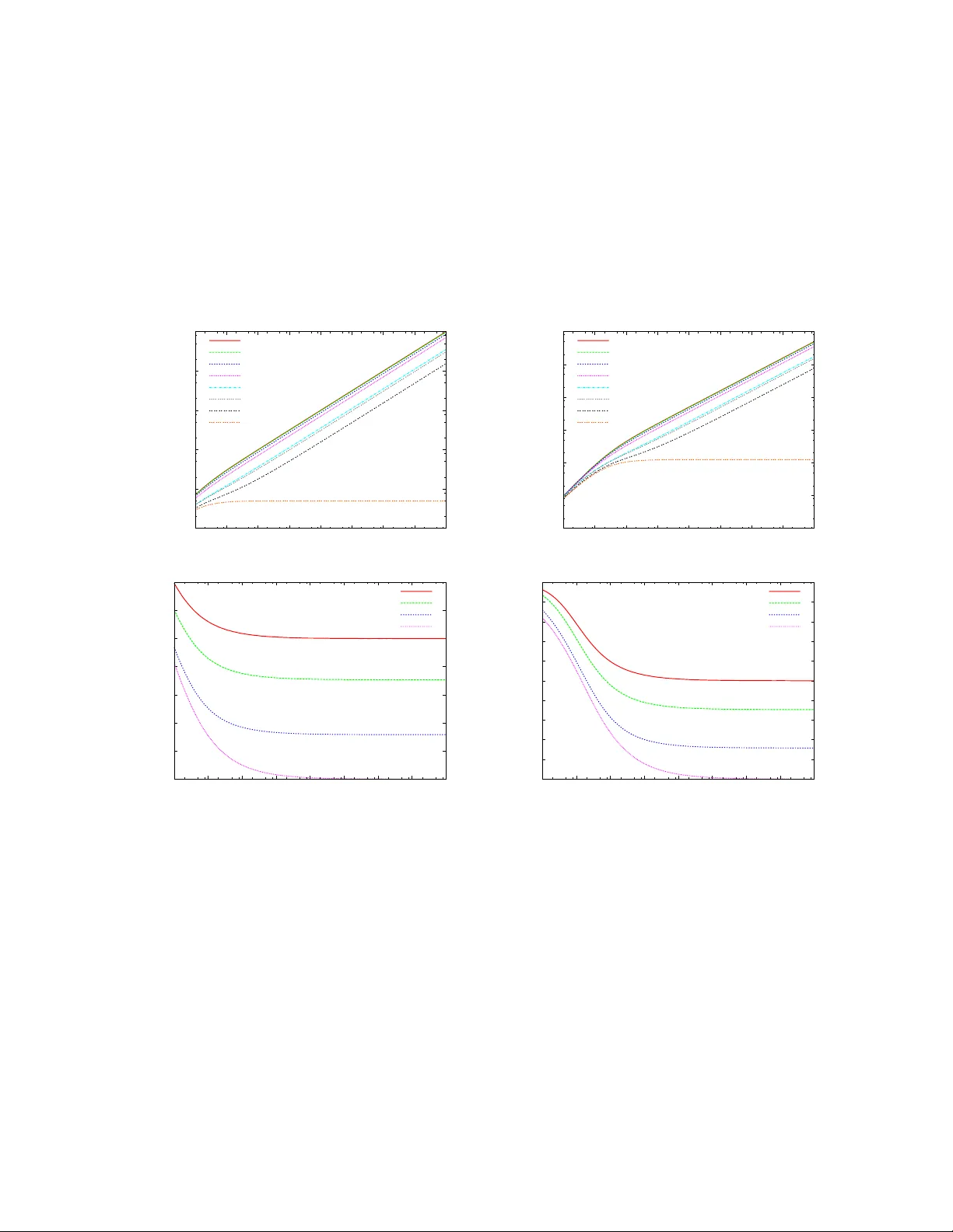
Get the Most out of Y our Sample: Optimal Unbiased Estimator s using P ar tial Inf ormation Edith Cohen A T&T Labs–Research 180 P ar k A ven ue Florham P ar k, NJ 07932, USA edith@research.att.com Haim Kaplan School of Computer Science T el A viv University T el A viv , Israel haimk@cs.tau.ac.il ABSTRA CT 1 Random sampling is an essential tool in the processing and transmission of data. It is used to summarize data too large to store or manipulate and meet resource constraints on bandwidth or battery power . Estimators that are applied to the sample facilitate fast approximate processing of queries posed over the original data and the value of the sample hinges on the quality of these estimators. Our work targets data sets such as request and trafﬁc logs and sensor measurements, where data is repeatedly collected over multiple instances : time periods, locations, or snapshots. W e are interested in queries that span multiple instances, such as distinct counts and distance measures over se- lected records. These queries are used for applications ranging from plan- ning to anomaly and change detection. Unbiased low-variance estimators are particularly effecti ve as the rela- tiv e error decreases with the number of selected record keys. The Horvitz- Thompson estimator , kno wn to minimize variance for sampling with “all or nothing” outcomes (which rev eals exacts v alue or no information on esti- mated quantity), is not optimal for multi-instance operations for which an outcome may provide partial information. W e present a general principled methodology for the deri vation of (Pareto) optimal unbiased estimators over sampled instances and aim to understand its potential. W e demonstrate signiﬁcant improvement in estimate accuracy of fundamental queries for common sampling schemes. 1. INTR ODUCTION Random sampling had become an essential tool in the handling of data. It is used to accommodate resource constraints on storage, bandwidth, energy , and processing power . Massi ve data sets can be too large to be stored long term or transmitted, sensor nodes collecting measurements are energy limited, and e ven when the full data is av ailable, computation of e xact aggre gates may be slo w and costly . The sample constitutes a summary of the original data sets that is small enough to store, transmit, and manipulate in a single location and yet supports computation of approximate queries over the orig- inal data. It is ﬂexible in that many types of queries are supported and that queries need not be known a priori [31, 39, 5, 4, 9, 25, 26, 2, 21, 2, 27, 13, 22, 10, 14]. Commonly , data has the form of multiple instances which are dispersed in time or location. Each instance corresponds to an as- signment of v alues to a set of identiﬁers (keys). The uni verse of ke y values is shared between instances but the values change. This data can be modeled as a numeric matrix of instances × keys. Instances can be snapshots of a database that is modiﬁed ov er time, measure- ments from sensors or of parameters tak en in different time periods, or number of requests for resources processed at multiple servers. Clearly , any scalable summarization algorithm of dispersed data must decouple the processing of dif ferent instances: the processing of one instance must not depend on values in other instances. 1 This is a full version of [15]. An important class of query primitiv es are functions with argu- ments that span v alues assumed by a k ey in multiple instances, such as quantiles (maximum, minimum, median) or the range (differ - ence between maximum and minimum). Sum aggr egates of these primitiv es over selected subsets of keys [32, 8, 17] include distinct element count (size of union), max-dominance and min-dominance norms [19, 20] and the Manhattan ( L 1 ) distance and are used for change or anomaly detection, similarity-based clustering, monitor- ing, and planning. See example in Figure 5 (A). Popular sampling scheme of a single instance are Poisson – where keys are sampled independently , bottom- k (order) [36, 12, 22, 13, 14] – where ke ys are assigned random rank values and the k small- est ranked keys are selected (as in weighted sampling without re- placement and priority sampling), and V A R O P T [10, 6] . The Horvitz Thompson ( H T ) estimator [29], based on in verse- probability weights, is a classic method for estimating subset-sums of values of keys: The estimate on the value of a key is 0 if it is not included in the sample and the ratio of its true value and the inclusion probability otherwise. The estimate on the sum of values of a subset of keys is the sum of estimates over sampled keys that are members of the subset. This estimator is unbiased and has minimum variance amongst unbiased nonnegativ e estimators. A variant of H T is used for bottom- k sampling [22, 38, 17]. Previous estimators we are aw are of for multi-instance functions are based on an adaptation of H T : a positive estimate is provided only on samples that revealed sufﬁcient information to compute the exact value of the estimated quantity . W e observe that such estimators may not be optimal for multi-instance functions, where outcomes can provide partial information on the estimated value. W e aim to understand the form and potential performance gain of better estimators. Contribution: W e characterize the joint sample distributions at- tainable for dispersed instances, that is, when processing of each instance may not depend on values of another . Our main contribution is a principled methodology for deriving optimal estimators for multi-instance functions, taking the sam- pling scheme as a given. The sample of each instance can be Poisson, V A R O P T , or bottom- k . Sampling can be weighted (in- clusion probability in the sample depends on the value) or weight- oblivious. The joint distribution (samples of different instances) can be independent or coor dinated . Coordination, achieved using random hash function, means that similar instances get similar sam- ples[3, 37, 34, 36, 5, 4, 9, 25, 26, 2, 13, 27, 14, 17] and can boost estimation quality of multi-instance functions [17, 18]. W e provide example derivations of optimal estimators for basic aggregations ov er common sampling distrib utions and demonstrate signiﬁcant gain, in terms of lower variance, over state-of-the-art estimators. Optimality is in a P areto sense with respect to v ariance: 1 any other nonnegati ve estimator with lower variance on some data must hav e higher variance on some other data. A key component in attaining optimality is the use of partial in- formation, which we motiv ate by the following simple scenario. Consider estimating the maximum of two v alues, v 1 and v 2 , sam- pled independently with respective probabilities p 1 and p 2 . W e can be certain about the value max( v 1 , v 2 ) only when both values are sampled, which happens with probability p 1 p 2 . The inv erse- probability weight is max( v 1 , v 2 ) / ( p 1 p 2 ) when both values are sampled and 0 otherwise and is an unbiased estimate. W e now observe that when exactly one of the values is sampled, we know that the maximum is at least that value, that is, we have meaning- ful partial information in the form of a positiv e lo wer bound on the maximum. W e will show how to exploit that and obtain a nonneg- ativ e and unbiased estimator with lower variance than the inv erse- probability weight. W e distinguish between independent weighted sampling schemes, according to the “reproducibility” of the randomization used: with Known (unknown) seeds the random hash functions used in sam- pling each instance are (are not) av ailable to the estimator . W e show that knowledge of seeds substantially increases estimation power: we provide nonnegativ e unbiased estimators for the max- imum when seeds are known and show that when seeds are un- known, there is no such estimator ev en when there are only two values and the domain is Boolean (in which case the maximum is OR of two bits). Our neg ativ e result for unkno wn seeds agrees with prior work that (implicitly) assume “unknown seeds, ” such as [7], who showed that most of the data needs to be sampled in order to obtain with constant probability small error estimate of distinct ele- ment count (which is a sum aggregate of O R ). “Known seeds” sam- pling, howe ver , can be easily incorporated when streaming or oth- erwise processing the full data set. W e demonstrate its beneﬁt when independent weighted samples of instances might be used post hoc for estimates of multi-instance queries. While reproducible ran- domization was extensi vely used as a means to coordinate samples, we believe that its potential to enhance the usefulness of indepen- dent weighted samples was not pre viously properly understood. Overview: Section 2 characterizes all sample distributions that are consistent with the constraints on summarization of dispersed val- ues. In Section 3 we propose methods to obtain optimal estimators which we apply in Sections 4-5 in example deriv ations. In Sec- tion 4 we consider weight-oblivious Poisson sampling of keys and independent sampling of instances and deriv e two Pareto optimal estimators for the maximum, one catering for data where values of a key are similar across instances and one where variation is large. W eighted sampling (with known seeds) is studied in Section 5 and we deriv e optimal estimators for the maximum and Boolean O R ov er two instances. Section 6 contains negativ e results for inde- pendently sampled instances with unknown seeds: W e show that there are no unbiased nonne gative estimators for maximum and for absolute difference, e ven when data is binary . In terms of an instances × keys data matrix, Sections 2–6 con- sider functions ov er the values v = ( v 1 , . . . , v r ) of a single key (i.e., column) in r dispersed instances. T o estimate sum aggre gates ov er multiple selected keys, we sum individual estimates for the selected keys. For example, to estimate distinct element count, we apply an O R estimator for each key and sum these estimates. Sec- tion 7 overvie ws the application of single-key estimators to sum aggregates. Applications to distinct count and max dominance are provided in Section 8. 2. SAMPLING DISPERSED V ALUES The data is represented by a vector v = ( v 1 , . . . , v r ) ∈ V where V ⊂ V 1 × · · · × V r and we are interested in the v alue of a function f ( v ) . Examples include the value v i of the i th entry , the  th largest entry  th ( v ) , the maximum max( v ) = max i ∈ [ r ] v i , the minimum min( v ) = min i ∈ [ r ] v i , the range R G ( v ) = max( v ) − min( v ) , and exponentiated range R G d ( v ) ≡ R G ( v ) d for d > 0 . The domain V can be the nonnegati ve quadrant of R r or { 0 , 1 } r . For a subset V 0 ⊂ V of data vectors we deﬁne f ( V 0 ) = inf { f ( v ) | v ∈ V 0 } and f ( V 0 ) = sup { f ( v ) | v ∈ V 0 } , the lowest and highest values of f on V 0 . W e see a random sample S ⊂ [ r ] of the entries of v . The sample distribution is subject to the constraint that the inclusion of i in S is independent of the values v j for j 6 = i . This is formalized as follows: There is a probability distribution T ov er a sample space Ω of predicates σ = ( σ 1 , . . . , σ r ) , where σ i has domain V i . The sample S ≡ S ( σ , v ) is a function of the predicate vector σ and the data vector v and includes i ∈ [ r ] if and only if σ i ( v i ) is true: i ∈ S ⇔ σ i ( v i ) . T w o special cases are: • W eight-oblivious sampling, where inclusion of i in S is indepen- dent of v i . The predicates σ i are constants ( 0 or 1 ) and entry i is sampled if and only if σ i = 1 (which happens with probability p i = E [ σ i ] ). • W eighted sampling where inclusion probability of each i is non- decreasing with v i (in particular , v i = 0 = ⇒ i 6∈ S ). W eighted sampling is important when the sample is used to esti- mate functions that increase with the data v alues. The predicates σ i are increasing functions that can be speciﬁed in terms of a transition threshold value τ i : i ∈ S ⇐ ⇒ σ i ( v i ) ⇐ ⇒ v i ≥ τ i . W e ﬁnd it con venient to specify weighted sampling distributions using non-decreasing functions τ i : [0 , 1] , i ∈ [ r ] and a random seed vector u ∈ [0 , 1] r so that u i ∈ [0 , 1] is uniformly distributed, with the interpretation that i ∈ S ⇐ ⇒ v i ≥ τ i ( u i ) . The inclusion probability of i is P R [ v i ≥ τ i ( u i )] = sup { u ∈ [0 , 1] | v i ≥ τ i ( u ) } . W eighted sampling is PPS (Probability Proportional to Size) when τ i = u i τ ∗ i , where τ ∗ is a ﬁxed vector . W ith PPS sampling, i is sampled with probability min { 1 , v i /τ ∗ i } . Independent (Poisson) sampling is when entries are sampled in- dependently , that is, the seeds u i are independent. In the general model, T is a product distribution and σ i is independent of all σ j for j 6 = i . Shared-seed (coordinated) sampling is when the entries of the seed vector are identical: u 1 = · · · = u r ≡ u where u ∈ [0 , 1] is selected uniformly at random. 2.1 Estimators An estimator ˆ f ( S ) of f ( v ) is a function applied to the outcome S (sampled entries and their values). The estimator depends on the domain V and distribution T . When sampling is weighted, we distinguish between two models, depending whether the seeds (the random predicate vector σ in the general model or the seed vector u ) are av ailable to the estimator . From the seed we can rev eal in- formation on values of entries that are not included in the sample: If i 6∈ S , we know that v i < τ i ( u i ) ( v i ∈ σ − 1 i (0) in the general model). W ith an outcome S , we associate a set V ∗ ( S ) ⊂ V of all data vectors consistent with this outcome. In the discrete case, 2 V ∗ ( S ) = { v ∈ V | P R [ S | v ] > 0 } . Otherwise, V ∗ ( S ) con- tains all vectors for which the probability density for the outcome is positive. When seeds are not known, V ∗ ( S ) contains v if and only if the probability density of S ( σ , v ) (where σ ∈ Ω ) is pos- itiv e for our outcome S . With known seeds, σ is av ailable, and hence v ∈ V ∗ ( S ) if and only if the outcome matches S ( σ , v ) . W e seek estimators with some or all of the follo wing properties: unbiased : for all v , E [ ˆ f | v ] = f ( v ) . nonne gative : ˆ f ≥ 0 . bounded variance : ∀ v , V A R [ ˆ f | v ] < ∞ . dominance: W e say that an estimator ˆ f (1) dominates ˆ f (2) if for all data vectors v , V A R [ ˆ f (1) | v ] ≤ V A R [ ˆ f (2) | v ] . An estimator ˆ f is dominant (P areto optimal) if there is no other unbiased nonnegativ e estimator ˆ f 0 that dominates ˆ f . monotone : Nonnegati ve and non-decreasing with information. If V ∗ ( S ) ⊂ V ∗ ( S 0 ) , then ˆ f ( S ) ≥ ˆ f ( S 0 ) . Unbiasedness is particularly desirable when estimating sums by summing indi vidual estimates: When unbiased and independent (or non-positiv ely correlated) estimates are combined, the relative er- ror decreases. Nonnegati vity is desirable when estimating a non- negati ve function f ≥ 0 , ensuring an estimate from the same do- main as the estimated quantity . If there is an estimator that domi- nates all others, it is the only optimal one. If there isn’t, we instead aim for Pareto optimality . Monotonicity is an intuitive smoothness requirement. 2.2 Horvitz Thompson estimator Suppose we are interested in estimating a function f ( v ) ≥ 0 under “all or nothing” sampling, where either the value is sampled and v is kno wn precisely or it is not sampled and we kno w nothing about f ( v ) . When the value is sampled, from the value v and the sample distrib ution we can compute the probability p that the v alue is sampled. The H T estimator [29] ˆ f ( H T ) of f ( v ) applies in verse pr obability weighting : ˆ f = 0 if the entry is not sampled and ˆ f = f ( v ) /p if it is sampled. This estimator is clearly nonneg ativ e, monotone, and unbiased: E [ ˆ f ] = (1 − p ) ∗ 0 + p f ( v ) p = f ( v ) . The v ariance is V A R [ ˆ f ] = f ( v ) 2  1 p − 1  . (1) The H T estimator is optimal in that V A R [ ˆ f ] is minimized for all v over all unbiased nonnegati ve estimators. Intuitively , this is be- cause an unbiased nonnegati ve estimator can not be positi ve (with nonzero probability) on outcomes that are consistent with f ( v ) = 0 and variance is minimized when using equal estimate when sam- pled. Multi-entry f . The application of inv erse-probability weights on multi-entry functions is more delicate. W e can use the set of out- comes for which S = [ r ] , that is all entries are sampled. For these outcomes we know the data v and from T we can determine P R [ S = [ r ] | v ] . The estimator is f ( v ) / P R [ S = [ r ] | v ] if S = [ r ] and 0 otherwise. This estimator is deﬁned when P R [ S = [ r ] | v ] > 0 . W ith weighted sampling, howe ver , “0” v alued entries are never sampled, so we may hav e P R [ S = [ r ]] = 0 when f ( v ) > 0 . A broader deﬁnition of in verse-probability estimators [17, 18] is with respect to a subset S ∗ of all possible outcomes (over Ω and V ). The outcomes S ∗ are those on which the estimator is positive. The estimator is deﬁned for S ∗ if there exist two functions f ∗ and p ∗ with domain S ∗ that satisfy the following: • for any outcome S ∈ S ∗ , for all v ∈ V ∗ ( S ) , f ( v ) = f ∗ ( S ) and P R [ S ∗ | v ] = p ∗ ( S ) . • for all v ∈ V with f ( v ) > 0 , P R [ S ∗ | v ] > 0 . The estimate is ˆ f ( S ) = 0 if S 6∈ S ∗ and ˆ f ( S ) = f ∗ ( S ) /p ∗ ( S ) otherwise. These functions and hence the estimator are unique for S ∗ if they e xist. When S ∗ is more inclusi ve, the respectiv e estima- tor has lower (or same) variance on all data. W e use the notation ˆ f ( H T ) for the estimator corresponding to the most inclusi ve S ∗ . A sufﬁcient condition for optimality of ˆ f ( H T ) is that for all outcomes S 6∈ S ∗ , f ( V ∗ ( S )) = 0 . 2.3 Necessary conditions for estimation In verse-probability estimators are unbiased, nonnegati ve (when f is) , and monotone. At most two different estimate values (zero and possibly a positiv e value) are possible for a giv en data vector and thus, variance is bounded. An inv erse-probability estimator, howe ver , exists only if for all data such that f ( v ) > 0 , there is positiv e probability of recovering f ( v ) from the outcome. This re- quirement e xcludes basic functions such as R G over weighted sam- ples: When the data has at least one positive and one zero entry , there is zero probability of recovering the exact value of R G ( v ) from the outcome. A nonneg ativ e, unbiased, and bounded-v ariance R G estimator , howe ver , was presented in [17, 18]. Aiming for a broader understanding of when an estimator with these properties exists, we deriv e some necessary conditions. For a set of outcomes, determined by a portion Ω 0 ⊂ Ω of the sample space and data vector v , we deﬁne V ∗ (Ω 0 , v ) = \ σ ∈ Ω 0 V ∗ ( S ( σ, v )) the set of all vectors that are consistent with all outcomes deter- mined by Ω 0 and v . For v and  , we deﬁne ∆( v ,  ) = 1 if ∀ σ , f ( S ( σ , v )) > f ( v ) −  and ∆( v ,  ) = 1 − sup  P R [Ω 0 ] | Ω 0 ⊂ Ω , f ( V ∗ (Ω 0 , v )) ≤ f ( v ) −   (2) otherwise. That is, we look for Ω 0 of maximum size such that if we consider all v ectors v 0 ∈ V ∗ (Ω 0 , v ) that are consistent with v on Ω 0 , the in- ﬁmum of f over V ∗ (Ω 0 , v ) is at most f ( v ) −  . W e deﬁne ∆( v ,  ) as the probability P R [Ω \ Ω 0 ] of not being in that portion. L E M M A 2.1. A function f has an estimator that is • unbiased and nonne gative ⇒ : ∀ v , ∀  > 0 , ∆( v ,  ) > 0 (3) • unbiased, nonne gative, and bounded variance ⇒ : ∀ v , ∆( v ,  ) = Ω(  2 ) . (4) • unbiased, nonne gative, and bounded ⇒ : ∀ v , ∆( v ,  ) = Ω(  ) . (5) P RO O F . The contribution of Ω 0 to the e xpectation of ˆ f must not exceed f ( V ∗ (Ω 0 , v )) . Because if it does, then ˆ f must assume ne g- ativ e values for v 0 ∈ V ∗ (Ω 0 , v ) with minimum f ( v 0 ) . Considering a maximum Ω 0 with f ( V ∗ (Ω 0 , v )) ≤ f ( v ) −  , its contribution to the expectation is at most f ( v ) −  and the contribution of the complement, which has probability ∆( v ,  ) , must be at least  . 3 If ∆( v ,  ) = 0 then this is not possible, so (3) follows. The ex- pectation of the estimator ov er the complement is at least  ∆( v , ) , thus (5) is necessary . The contribution to the variance of that com- plement is at least ∆( v ,  )   ∆( v ,  ) − f ( v )  2 which implies (4) is necessary . 3. P ARETO OPTIMAL ESTIMA TORS W e formulate sufﬁcient conditions for Pareto optimality , which form the basis of our estimator deriv ations. W e start by seeking Pareto optimal estimators deﬁned with re- spect to an order ≺ over the set V of all possible data vectors and minimizing variance in an order-respecting way: The variance of the estimator for a data vector v is minimized conditioned on val- ues it assigned to outcomes consistent with vectors that precede v . This setup naturally yields estimators that are Pareto optimal. Moreov er , by selecting an order ≺ so that more likely vectors ap- pear earlier, we can tailor the estimator according to properties of the data. Order -based optimality ˆ f ( ≺ ) : The ﬁrst estimator we present, ˆ f ( ≺ ) , is the solution of a simple set of equations. A solution may not ex- ist, but when it does, it is unique and P areto optimal. W e map an outcome S to its ≺ -minimal consistent data vector φ ( S ) ≡ min ≺ V ∗ ( S ) (we assume it is well deﬁned). W e say that S is determined by the data vector v ≡ φ ( S ) and that v is the de- termining vector of S . An outcome S precedes v if it is determined by z ≺ v . For continuous spaces V and S , we extend some assumptions on the mapping φ from the discrete case: (i) For all v , φ − 1 ( v ) is either empty or has positive probability , (ii) any subset of φ − 1 ( v ) with zero probability for data v also has zero probability for data z  v , and (iii) any positiv e-probability set of outcomes consistent with v and determined by preceding vectors must include a positiv e probability subset of φ − 1 ( z ) for some z ≺ v . For each vector v , ˆ f ( ≺ ) has the same v alue on all outcomes S 0 ≡ φ − 1 ( v ) determined by v . Slightly abusing notation, we de- ﬁne ˆ f ( ≺ ) ( v ) ≡ ˆ f ( ≺ ) ( S ) for S ∈ S 0 to be that value. W e express ˆ f ( ≺ ) ( v ) as a function of ˆ f ( ≺ ) on the outcomes S 0 that precede v . The dependence on preceding outcomes S 0 is through their contribution f 0 to the expectation of the estimate of f ( v ) . The estimate value ˆ f ( ≺ ) ( v ) is as follows: If P R [ S 0 | v ] = 0 and f ( v ) = f 0 , ˆ f ( ≺ ) ( v ) ← 0 . If P R [ S 0 | v ] = 0 and f ( v ) 6 = f 0 , we declare failure. Else, ˆ f ( ≺ ) ( v ) ← f ( v ) − f 0 P R [ S 0 | v ] . (6) From the in verse-probability weights principle, this choice of ˆ f ( S ) for S ∈ S 0 minimizes the variance V A R [ ˆ f | v ] for data vector v conditioned on the values ˆ f : S 0 . When the order ≺ enumerates all data vectors (all data vectors hav e ﬁnite position in the order), we can compute ˆ f ( ≺ ) algorithmi- cally: Algorithm 1 processes data vectors sequentially in increasing ≺ order and computes ˆ f ( v ) when v is processed. These constraints ha ve no solution when for some v , f 0 < f ( v ) and P R [ S 0 | v ] = 0 . Moreo ver , if f 0 > f ( v ) , there is no nonnega- tiv e solution. When a solution f ( ≺ ) is well deﬁned, howe ver , it is unbiased and Pareto optimal Algorithm 1 ˆ f ( ≺ ) Require: ≺ is an order on V 1: S 0 ← ∅  set of processed outcomes 2: V 0 ← ∅  set of processed data vectors 3: while V 0 6 = V do 4: v ← min ≺ ( V \ V 0 )  A minimum unprocessed vector 5: f 0 ← E [ ˆ f ( ≺ ) ( S ) |S 0 , v ] P R [ S 0 | v ]  Contribution of preceding outcomes to the estimate of f ( v ) 6: S 0 ← { S | v ∈ V ∗ ( S ) } \ S 0  Unprocessed outcomes consistent with v 7: if P R [ S 0 | v ] = 0 then 8: if f ( v ) 6 = f 0 then return “failure”  No unbiased estimator 9: else 10: ˆ f ← 0 11: ∀ S ∈ S 0 , ˆ f ( ≺ ) ( S ) ← 0 12: else 13: ˆ f ← f ( v ) − f 0 P R [ S 0 | v ] 14: ∀ S ∈ S 0 , ˆ f ( ≺ ) ( S ) ← ˆ f 15: V 0 ← V 0 ∪ { v } 16: S 0 ← S 0 ∪ S 0 L E M M A 3.1. When ˆ f ( ≺ ) is well deﬁned, it is unbiased and P ar eto optimal. P RO O F . Pareto optimality: Consider an estimator ˆ f ( ≺ ) such that for some v , ˆ f 6 = ˆ f ( ≺ ) on a set of outcomes D such that P R [ D | v ] > 0 . Let v be ≺ -minimal with this property , and let S 0 and S 0 be as in our constraints, with respect to v . From deﬁnition of φ , the set D (or a same-probability subset of it) must be contained in S 0 . From ≺ -minimality of v and our assumptions for continuous spaces, we must have E [ ˆ f ( ≺ ) : |S 0 ] = E [ ˆ f |S 0 ] and hence ˆ f ( ≺ ) : S 0 6 = ˆ f : S 0 . The value assigned by ˆ f ( ≺ ) on the outcomes S 0 is the unique choice which minimizes the variance of v subject to ˆ f ( ≺ ) : S 0 , in the sense that any estimator that differs on a positive probability subset of S 0 will have strictly higher variance. Hence, V A R [ ˆ f | v ] > V A R [ ˆ f ( ≺ ) | v ] and thus ˆ f can not dominate ˆ f ( ≺ ) . Unbiasedness follows from the choice of ˆ f ( ≺ ) on the outcomes S 0 in (6) (line 13 of Algorithm 1): E [ ˆ f ( ≺ ) ] = E [ ˆ f ( ≺ ) |S 0 ] P R [ S 0 ] + E [ ˆ f ( ≺ ) |S 0 ] P R [ S 0 ] = f ( v ) . T wo v ectors v ≺ z are dependent with respect to ≺ if P R [ φ − 1 ( v ) | z ] > 0 . Consider now a partial order ≺ 0 deriv ed from ≺ by only retain- ing relations between dependent vectors. Then all linearizations of ≺ 0 hav e the same mapping of outcomes to determining v ectors and thus, the resulting order-based estimators are identical. Conv ersely , when a partial order ≺ 0 has the property that for all outcomes S , min ≺ V ∗ ( S ) is unique, we can specify the estimator f ( ≺ 0 ) with respect to it (same as using any linearization). L E M M A 3.2. The estimator ˆ f ( ≺ ) is monotone if and only if for any outcome S and v ∈ V ∗ ( S ) , the estimate on outcomes deter- mined by v is at least ˆ f ( ≺ ) ( S ) : ˆ f ( ≺ ) is monotone ⇐ ⇒ ∀ S, ∀ v ∈ V ∗ ( S ) ˆ f ( ≺ ) ( v ) ≥ ˆ f ( ≺ ) ( S ) . P RO O F . An outcome S 0 with V ∗ ( S 0 ) = { v } has V ∗ ( S 0 ) ⊂ V ∗ ( S ) and is determined by v . From monotonicity , we must have ˆ f ( ≺ ) ( v ) ≥ ˆ f ( ≺ ) ( S ) . Conv ersely , consider two outcomes S and S 0 such that V ∗ ( S ) ⊂ V ∗ ( S 0 ) . Let v 0 be the determining v ector of S 0 and v be the determining vector of S . W e have that v ∈ S 0 , hence ˆ f ( ≺ ) ( v ) = ˆ f ( ≺ ) ( S ) ≥ ˆ f ( ≺ ) ( S 0 ) . 4 For cing nonnegativity ˆ f (+ ≺ ) : When the constraints specifying f ( ≺ ) hav e no nonnegativ e solution, we can explicitly constrain the setting of ˆ f ( ≺ ) : S 0 to ensure that nonnegativity is not violated on successive vectors: min X S ∈S 0 P R [ S | v ]( ˆ f ( S ) − f ( v )) 2 (7) X S ∈S 0 P R [ S | v ] ˆ f ( S ) = f ( v ) − f 0 (8) ∀ v 0  v X S ∈ S 0 ∪ S 0 ˆ f ( S ) P R [ S | v 0 ] ≤ f ( v 0 ) . (9) W e minimize variance (7) subject to unbiasedness (8) and not vio- lating nonnegativity to any v 0  v (9). The resulting estimator is Pareto optimal if the solution of the system is unique. A solution ˆ f (+ ≺ ) satisfying nonnegati vity constraints is identi- cal to ˆ f ( ≺ ) when the latter is deﬁned and nonneg ativ e. With ˆ f (+ ≺ ) formulation, the constraints (9) can make two vectors v and z de- pendent also when both sets of outcomes φ − 1 ( v ) and φ − 1 ( z ) have positiv e probability for some data vector y that succeeds both v and z . This is because when v precedes z , the constraints (9) due to y are less tight. As with ˆ f ( ≺ ) , we can equi valently deﬁne ˆ f (+ ≺ ) with respect to a partial order ≺ 0 deriv ed from ≺ by including only relations between dependent data vectors and all linearizations of ≺ 0 . Ordered partition ˆ f ( U ) : The order-based formulations, ho wev er, in particular the more constrained ˆ f (+ ≺ ) , can preclude symmetric estimators. Symmetric estimators are naturally desirable when f is symmetric (in variant under permuting coordinates). When two symmetric vectors are dependent under ≺ , the member that ≺ - precedes the other can hav e a strictly lower variance. W e therefore seek a more relaxed formulation that will allow us to balance the variance of symmetric v ectors. W e consider a setup where data vectors are partitioned into or- dered batches U = { U 0 , U 1 , . . . } . The estimator ˆ f ( U ) prioritizes earlier batches b ut “balances” the v ariance between vectors that are members of the same batch. That is, the estimator is locally P ar eto optimal for each U i : given ˆ f : S 0 , unbiasedness (8) for all v ∈ U i and nonnegati vity (9) for all v 0 ∈ U >i . That is, under these con- straints, there is no other setting of ˆ f on S 0 with smaller or equal variance for all vectors in U i , and a strictly smaller variance for at least one vector . The estimator ˆ f ( U ) is Pareto optimal if at each step h , when ﬁxing the variance of all vectors in U h , the solution is unique. Symmetry (inv ariance to permutation of entries) can be achiev ed by including all symmetric data vectors in the same part and using a symmetric locally optimal estimator . This is formulated in Algorithm 2, which processes U i at step i , setting the estimator on all outcomes consistent with U i and not consistent with any v ector in U j for j < i . 4. POISSON: WEIGHT -OBLIVIOUS W e now consider estimating f ( v ) when sampling of entries is weight-oblivious and Poisson: entry i ∈ [ r ] is sampled indepen- dently with probability p i > 0 . The outcome S ⊂ [ r ] includes the sampled entries, and for each sampled entry i ∈ S , the value v i . The in verse-probability estimate ˆ f ( H T ) ( S ) = f ( v ) / Q i ∈ [ r ] p i , when S ≡ [ r ] (all entries are sampled), and ˆ f ( H T ) ( S ) = 0 other- Algorithm 2 ˆ f ( U ) Require: U 0 , U 1 , . . . is a partition of V 1: S 0 ← ∅  set of processed outcomes 2: for h = 0 , 1 , 2 , . . . do  h is the index of current part to process 3: S 0 ← { S | U h ∩ V ∗ ( S ) 6 = ∅} \ S 0  Unprocessed outcomes consistent with U h 4: Compute a locally optimal estimator for U h , extending ˆ f on S 0 , and satisfying ∀ v 0 , X S ∈ S 0 ∪ S 0 ˆ f ( S ) P R [ S | v 0 ] ≤ f ( v 0 ) . 5: S 0 ← S 0 ∪ S 0 wise, is deﬁned for all f and from (1) has variance V A R [ ˆ f ( H T ) ] = f ( v ) 2 1 Q i ∈ [ r ] p i − 1 ! . (10) This estimator is the optimal in verse probability estimator for quan- tiles and range: The set of outcomes S ∗ which contains all out- comes with | S | = r is the most inclusiv e set for which we can determine both the v alue f ( v ) and P R [ S ∗ | v ] (see Section 2.2). The estimators ˆ R G ( H T ) ( r = 2 ) and ˆ min ( H T ) are even (Pareto) opti- mal: this is because any nonnegati ve estimator must have ˆ f ( S ) = 0 on outcomes v consistent with data vectors with f ( v ) = 0 , which includes all outcomes with | S | < r for these two functions. Con- sidering all estimators that assume positi ve v alues only when | S | = r , v ariance is minimized when using a ﬁxed value. The estimator ˆ f ( H T ) , howe ver , is not optimal for all other quantiles (  th when  < r ) or for R G when r > 2 . W e present optimal estimators for max and Boolean O R : the monotone estimators ˆ max ( L ) and ˆ O R ( L ) which prioritize dense data vectors and the estimators ˆ max ( U ) and ˆ O R ( U ) which prioritize sparse vectors. 4.1 Estimator ˆ max ( L ) W e compute the estimator f ( ≺ ) (Algorithm 1) with respect to the following partial order ≺ : The data vector 0 precedes all others, that is ∀ v ∈ V , 0 ≺ v . Otherwise, ≺ corresponds to the numeric order on L ( v ) ≡ |{ j ∈ [ r ] | v j < max i ∈ [ r ] v i }| (the number of entries strictly lower than the maximum one): v ≺ w ⇐ ⇒ L ( v ) < L ( w ) . For an outcome S , the set V ∗ ( S ) includes all vectors that agree with the outcome on sampled entries: v 0 ∈ V ∗ ( S ) ⇐ ⇒ ∀ i ∈ S, v 0 i = v i . The determining vector φ ( S ) of an outcome S is min ≺ V ∗ ( S ) : φ ( S ) = 0 if ∀ i ∈ S, v i = 0 (In particular if S = ∅ ). If S 6 = ∅ , φ ( S ) j ≡ v j if j ∈ S and φ ( S ) j = max i ∈ S v i otherwise. The mapping φ ( S ) is well deﬁned by ≺ , which means that the estimator f ( ≺ ) (if deﬁned) is unique. Because ≺ is symmetric (inv ariant to permutation of entries), so is f ( ≺ ) . Our choice of ≺ aims at obtaining a monotone estimator through conservati ve (low) estimate values: The determining vector of an outcome S has all unsampled entries set to the maximum value of a sampled entry (this value is also the lower bound f ( V ∗ ( S 0 )) ). The optimal estimate value for this vector on S would be lower than if we had a determining vector with lower entries and same maximum because the outcome on such a vectors is more likely to hav e a lower maximum sampled entry , meaning a lower estimate 5 on such outcomes which needs to be compensated for by a higher estimate on S . For the minimum vector 0 , there are no preceding outcomes ( S 0 = ∅ ) and we can directly compute ˆ max ( L ) ( 0 ) (the estimate for all outcomes that have φ ( S ) = 0 ), obtaining ˆ max ( L ) = 0 on all outcomes S such that ∀ i ∈ S , v i = 0 . W e can no w proceed and compute the estimator for all outcomes S with determining vector v such that L ( v ) = 0 , that is, outcomes where at least one entry is sampled, has positiv e v alue, and all other sampled entries have the same value: ∀ i ∈ S , v i = max i ∈ S v i > 0 . The probability of such an outcome given data vector v with L ( v ) = 0 is the probability that at least one entry is sampled: 1 − Q i ∈ [ r ] (1 − p i ) and the estimate value is accordingly ˆ max ( L ) = max i ∈ S v i 1 − Q i ∈ [ r ] (1 − p i ) . (11) Maximum over two instances ( r = 2 ). W e hav e ˆ max ( L ) = 0 on outcomes consistent with data (0 , 0) and from (11) ˆ max ( L ) = max i ∈ S v i p 1 + p 2 − p 1 p 2 for outcomes consistent with data with two equal pos- itiv e entries ( S = { 1 } , S = { 2 } , or S = { 1 , 2 } and v 1 = v 2 = v ). W e now consider data vectors where v 2 < v 1 (other case v 1 < v 2 is symmetric). The estimate is already computed on outcomes where exactly one entry is sampled. These and the empty outcome are in S 0 . The outcomes S 0 are those where both entries are sampled, and hence P R [ S 0 ] = p 1 p 2 . T o be unbiased, the estimate x must satisfy the linear equation (line 13 of Algorithm 1): max { v 1 , v 2 } = p 1 p 2 x + + p 1 (1 − p 2 ) v 1 p 1 + p 2 − p 1 p 2 + p 2 (1 − p 1 ) v 2 p 1 + p 2 − p 1 p 2 . Solving and summarizing we obtain: Outcome S ˆ max ( L ) ( S ) S = ∅ : 0 S = { 1 } : v 1 p 1 + p 2 − p 1 p 2 S = { 2 } : v 2 p 1 + p 2 − p 1 p 2 S = { 1 , 2 } : max( v 1 ,v 2 ) p 1 p 2 − (1 /p 2 − 1) v 1 +(1 /p 1 − 1) v 2 p 1 + p 2 − p 1 p 2 . Expressing the estimator as a function of the determining v ector , assuming v 1 ≥ v 2 (other case is symmetric), we obtain: ˆ max ( L ) ( v ) = v 1 1 p 1 ( p 1 + p 2 − p 1 p 2 ) − v 2 1 − p 1 p 1 ( p 1 + p 2 − p 1 p 2 ) (12) L E M M A 4.1. The estimator ˆ max ( L ) is P areto optimal, mono- tone, nonne gative, and dominates the estimator ˆ max ( H T ) . P RO O F . Pareto optimality follo ws from the ˆ f ( ≺ ) deriv ation. For monotonicity , we observe that determining vectors of more infor- mativ e outcomes (outcomes with more entries sampled) have an equal-or-lar ger maximum entry v 1 or an equal-or -smaller minimum entry v 2 , which clearly holds as the coefﬁcient of v 1 in (12) is pos- itiv e and that of v 2 is negati ve. Nonnegati vity follows from mono- tonicity and the fact that the estimate is 0 when S = ∅ . The estimator ˆ max ( H T ) assumes v alues 0 or max( v 1 ,v 2 ) p 1 p 2 and thus maximizes v ariance amongst all unbiased estimators with values in the same range. Hence, to establish dominance over ˆ max ( H T ) , it sufﬁces to sho w that on data v , ˆ max ( L ) ( v ) ≤ max( v 1 ,v 2 ) p 1 p 2 , which is immediate from (12). Multiple instances: ˆ max ( L ) for r ≥ 2 . A sorting permutation of a vector v is a permutation π of [ r ] such that v π 1 ≥ · · · ≥ v π r . W e use the notation π ( v ) = ( v π 1 , . . . , v π r ) . W e pro ve that the estimator ˆ max ( L ) applied to an outcome S can be e xpressed as a linear combination of the sorted entries of the de- termining vector φ ( S ) . The coefﬁcients depend on an accordingly permuted probability vector . When there are multiple entry of equal value, the sorting permutation is not unique. W e show , howe ver , that the estimator is in variant to the particular sorting permutation used. T H E O R E M 4.1. ˆ max ( L ) ( S ) = X i ∈ [ r ] α i, π ( p ) φ ( S ) π i , (13) wher e π is the sorting permutation of φ ( S ) and α i, q ar e rational expr essions in q 1 , . . . , q r that ar e always deﬁned when q i ∈ (0 , 1] . Mor eover , the coefﬁcients’ pr eﬁx sums A h, p ≡ h X i =1 α i, p (14) ar e symmetric rational e xpressions for p i for i ∈ [ h ] and for p i for i ∈ [ r ] \ [ h ] . P RO O F . W e ﬁrst show that the symmetry property of the pre- ﬁx sums implies that the estimate does not depend on the choice of sorting permutation (when it is not unique). It sufﬁces to show this for a sorted v such that v j ≡ v j +1 and show that when sym- metry holds, the estimator is the same for the identity permutation (1 , . . . , r ) and the permutation (1 , . . . , j − 1 , j + 1 , j, j + 1 , . . . , r ) (exchanging positions j and j + 1 ). Both are sorting permutations of v ). The argument can be applied repeatedly if there are more than two equal entries. Let v be sorted and let δ i ≡ v i +1 − v i for i = ∈ [ r − 1] . W e can rewrite (13) as r X i =1 α i, p v i = A r, p v 1 − r − 1 X i =1 δ i A i, p When δ j = 0 , let p and p 0 respectiv ely be the original and per- muted v ectors with p j and p j +1 exchanged. By symmetry , A i, p = A i, p 0 for i ∈ [ r ] \ { j } . But δ j = 0 , and hence the estimator is the same with both permutations. W e now show that the estimator has the form (13) and that the preﬁx sums satisfy the symmetry property . For v with sorting per- mutation π and L ( v ) = k , we can rewrite (13) as h X i =1 α i, π ( p ) v π i (15) = v π 1 A r − k , π ( p ) + r X i = r − k +1 ( A i, π ( p ) − A i − 1 , π ( p ) ) v π i . For all outcomes S consistent with v , L ( φ ( S )) ≤ L ( v ) ≤ k . Thus, the estimator for data v is fully speciﬁed by A h, π ( p ) where h ≥ r − L ( v ) . W e show by induction on k ≥ 0 , that the estimator can be ex- pressed in this form for data vectors with L ( v ) ≤ k . For the base case of the induction ( k = 0 ), it sufﬁces to specify the rational ex- pression A r, p . By substituting a determining vector with all entries equal in (13) and equating with (11), we obtain A r, p = 1 1 − Q i ∈ [ r ] (1 − p i ) (16) 6 speciﬁes max ( L ) ( v ) for all determining vectors v such that L ( v ) = 0 (all entries are equal and positive) and thus speciﬁes the estima- tor correctly for all data vectors with L ( v ) = 0 . Symmetry clearly holds as A r, π ( p ) is independent of the particular permutation π . In the induction step we assume that the rational expressions A i, p are well deﬁned and satisfy symmetry for all i ≥ r − k and all p , that is, (15) is equal to max ( L ) when L ( φ ( S )) ≤ k and hence the estimator is speciﬁed for data with L ( v ) ≤ k . W e then specify A r − k − 1 , p by relating it through a linear equation to higher preﬁx sums. This fully speciﬁes the estimator for data with L ( v ) = k + 1 . Symmetry properties of A r − k − 1 , π ( p ) (showing it is symmetric in { p 1 , . . . , p r − k − 1 } and in { p r − k , . . . , p r } ) follow from the sym- metry in the equation and assumed symmetry of the higher preﬁx sums. W e no w express A r − k − 1 , p as a linear combination of preﬁx sums of the form A h, π 0 ( p ) where h ≥ r − k and [ r − k ] ⊂ { π 0 1 , . . . , π 0 h } . Consider a vector z such that L ( z ) = k + 1 and entries are sorted in nonincreasing order (the sorting permutation is the identity , and this is without loss of generality as we can permute p accordingly). W e show that there is a (unique) value of A r − k − 1 , p that results in an unbiased estimate for z . This value turns out to be independent of z (works for all vectors with L ( v ) = k + 1 and same permutation of sorted entries). When solved parametrically , this is a rational expression in p 1 , . . . , p r that satisﬁes the symmetry property . The vector z has z 1 = · · · = z r − k − 1 ≡ Z and z r ≤ · · · ≤ z r − k < Z . Consider the vector z 0 that is equal to z on all entries except that z 0 r − k ≡ Z . Clearly L ( z 0 ) = k and therefore, by induc- tion, the estimate for z 0 is unbiased, that is, has expectation Z on data z 0 . W e relate outcomes for different data vectors that correspond to the same sample σ ∈ 2 [ r ] which is the set of sampled entries. The vectors z 0 and z have the same determining vectors, and thus, the same estimate on all samples where σ r − k = 0 (do not include the entry r − k ). Therefore, the estimate is unbiased on z , if and only if the expectation for data z is equal to the expectation for data z 0 ov er samples where σ r − k = 1 (entry r − k is sampled). W e consider the difference in the contribution to the estimate of a sample σ that includes r − k on the data vectors z and z 0 . If none of the entries [ r − k − 1] is sampled, the determining vectors dif fer on the ﬁrst h ≥ r − k entries (where h is equal to r − k plus the number of unsampled entries in [ r − k + 1 , r ] ). The value of the determining vector on the ﬁrst h entries is Z when the data is z and Z 0 when the data is z 0 . There is a sorting permutation π 0 for both determining vectors which depends only on the sample σ (works for all choices of z and respective z 0 : it has all unsam- pled entries in sorted order , followed by entry r − k , and then by other sampled entries in sorted order. Thus, the difference in the contribution to the estimate is A h, π 0 ( p ) ( Z − Z 0 ) . If at least one of the entries [ r − k − 1] is sampled, then the determining vectors are identical on the ﬁrst h − 1 entries (value is Z ), differ on entry h (the v alue is Z when data is z and Z 0 when z 0 ) and identical on remaining entries (values smaller than Z 0 ). Again, there is a common sorting permutation π 0 for the determining vector of all choices of z and of z 0 : it contains the ﬁrst r − k − 1 entries and unsampled entries in [ r − k + 1 , r ] , all in sorted order , followed by r − k , and then sampled entries in [ r − k + 1 , r ] in sorted order (note that it is the same permuta- tion we used for the case where none of the entries [ r − k − 1] are sampled). Thus, the difference in the contribution to the estimate is α h, π 0 ( p ) ( Z − Z 0 ) = ( A h, π 0 ( p ) − A h − 1 , π 0 ( p ) ) (Z-Z’). The only samples for which h = r − k is when all entries in [ r − k , r ] are sampled. In this case the determining v ectors are the respectiv e data vectors and the sorting permutation of the determining vec- tor is the identity . Thus the only “unknown” is A r − k − 1 , p and it appears, when replacing α r − k , p = A r − k , p − A r − k − 1 , p . Recall that for the estimate for z to be unbiased, the expectation of these dif ferences over samples must be 0 . The expectation is the sum ov er samples σ of the probability of the sample P R [ σ ] = Y i ∈ [ r ] p σ i i (1 − p i ) 1 − σ i multiplied by the dif ference. By equating with 0 we obtain a linear equation with one variable A r − k − 1 , p , which must have a unique solution. Since all terms are multiplied by ( Z − Z 0 ) , it factors out. The equation and solution A r − k − 1 , p are independent of z . There- fore, the estimate is unbiased for all data vectors z with L ( z ) = k + 1 . W e now write the equations explicitly , using the notation π σ = (1 , . . . , r − k − 1 , { i = r − k + 1 , . . . , r | σ i = 0 } , r − k , { i = r − k + 1 , . . . , r | σ i = 1 } ) h σ = r − k + r X i = r − k +1 σ i for the sorting permutation and h value used with the sample σ . 0 = X σ ∈ 2 [ r ] | σ r − k =1 P R [ σ ]  I ( r − k − 1 X i =1 σ i = 0) A h σ , π σ ( p ) + I ( r − k − 1 X i =1 σ i ≥ 1) α h σ , π σ ( p )  where I is the indicator function. W e can express the equation in terms of the projection σ of the sample σ on entries K = [ r − k + 1 , r ] . W e combine terms with identical projection while noting that π σ ≡ π σ and h σ ≡ h σ depend only on the projection. W e eliminate common terms and obtain: 0 = X σ ∈ 2 K P R [ σ ]  r − k − 1 Y i =1 (1 − p i ) A h σ , π σ ( p ) + (1 − r − k − 1 Y i =1 (1 − p i ))( A h σ , π σ ( p ) − A h σ − 1 , π σ ( p ) )  = X σ ∈ 2 K P R [ σ ] (17)  A h σ , π σ ( p ) − (1 − r − k − 1 Y i =1 (1 − p i )) A h σ − 1 , π σ ( p ) )  For k = 0 , K = ∅ and thus there is only one term. The equation relates A r − 1 , p and A r, p , yielding A r − 1 , p = A r, p (1 − Q r − 1 i =1 (1 − p i )) (18) For k = 1 , K = { r } and hence there are two terms, according 7 to the value of σ r : 0 = (1 − p r )  A r, p − (1 − r − 2 Y i =1 (1 − p i )) A r − 1 , ( p 1 ,...,p r − 2 ,p r ,p r − 1 )  + p r  A r − 1 , p − (1 − r − 2 Y i =1 (1 − p i )) A r − 2 , p  Therefore, A r − 2 , p = A r − 1 , p + A r − 1 , p 0 − A r, p 1 − Q r − 2 i =1 (1 − p i ) where p 0 = ( p 1 , . . . , p r − 2 , p r , p r − 1 ) . W e conjecture that ˆ max ( L ) is monotone, nonnegati ve, and dom- inates ˆ max ( H T ) . W e veriﬁed these properties for r ≤ 4 with uni- form p , using the follo wing lemma and explicit computation of the coefﬁcients. L E M M A 4.2. T o establish monotonicity , nonne gativity , and dom- inance of ˆ max ( L ) over ˆ max ( H T ) it sufﬁces to show that α i < 0 for i > 1 and that α 1 ≤ 1 / Q i ∈ [ r ] p i . P RO O F . T o establish monotonicity , consider two types of ma- nipulations of a determining vector: increasing some of its maxi- mum entries or decreasing a maximum entry in case the maximum entry is not unique. Now , for any data v and outcomes S 1 ⊂ S 2 ( S 2 contains all entries sampled in S 1 and more), the determining vector of S 2 can be obtained from that of S 1 using such operations. For monotonicity , we need to sho w that the estimate value obtained for v on outcome S 2 is at least that of S 1 , equivalently , that these manipulations can only increase ˆ max ( L ) . For the second manip- ulation, it sufﬁces to show that α i < 0 for i > 1 . F or the ﬁrst manipulation, it suf ﬁces to show that P i j =1 α j > 0 for all i ≥ 1 . Since we know that P i ∈ [ r ] α i > 0 , this is implied by α i < 0 for i > 1 . Nonnegati vity follows from monotonicity and the base case of estimate value 0 when there are no sampled entries. T o establish dominance over ˆ max ( H T ) , given monotonicity , it sufﬁces to show that α 1 ≤ 1 / Q i ∈ [ r ] p i . This means that all ˆ max ( L ) estimates on a given data vector v are at most max( v ) Q i ∈ [ r ] p i , which is the ˆ max ( H T ) estimate. The H T estimate has maximum variance amongst all unbiased estimators that assume values in the range  0 , max( v ) Q i ∈ [ r ] p i  . Hence, V A R [ ˆ max ( L ) ] ≤ V A R [ ˆ max ( H T ) ] . These expression can be use to compute the estimator , but the number of dif ferent preﬁx-sums gro ws exponentially with the num- ber of distinct probabilities in the k sufﬁx of p . W e give speciﬁc consideration to uniform probabilities. Uniform p . When p = p 1 = p 2 = . . . = p r , we can use α i, p ≡ α i,p and A i, p ≡ A i,p for the coefﬁcients in (13) and their respectiv e preﬁx sums. For a gi ven p , we only need r different v al- ues, A i,p for i ∈ [ r ] , to specify the estimator . W e omit p from the subscript for brevity . W e show that for a ﬁxed p , the estimator can be computed in time quadratic in the dimension. T H E O R E M 4.2. The estimator , for a given p , can be computed in O ( r 2 ) time using the r elation A r,p = 1 1 − (1 − p ) r (19) A r − k − 1 = (20) A r − k + k X ` =1  k `   1 − p p  `  A r − k + ` − (1 − (1 − p ) r − k − 1 ) A r − k + ` − 1  1 − (1 − p ) r − k − 1 P RO O F . Using uniform p , (16) simpliﬁes to (19). The equation (17) simpliﬁes to 0 = k X ` =0 k  ! p k − ` (1 − p ) ` · (21)  A r − k + ` − (1 − (1 − p ) r − k − 1 ) A r − k + ` − 1  W e obtain (20) by expressing A r − k − 1 as a function of A h for h ≥ r − k . This relation is a triangular system of linear equations and allows us to compute the estimator (the coef ﬁcients α i,p for i ∈ [ r ] for a giv en p ) in time O ( r 2 ) . W e compute the parametric form of the higher preﬁx sums: A r = 1 1 − (1 − p ) r A r − 1 = A r 1 1 − (1 − p ) r − 1 A r − 2 = A r − 1 1 + (1 − p ) r − 1 1 − (1 − p ) r − 2 For r = 2 , we obtain A 2 = 1 p (2 − p ) A 1 = 1 p 2 (2 − p ) Using α 2 = A 2 − A 1 and α 1 = A 1 , we obtain the estimator α =  1 p 2 (2 − p ) , − 1 − p p 2 (2 − p )  (22) For r = 3 , we obtain A 3 = 1 p ( p 2 − 3 p + 3) A 2 = 1 p 2 ( p 2 − 3 p + 3)(2 − p ) A 1 = 2 + p 2 − 2 p p 3 ( p 2 − 3 p + 3)(2 − p ) Using α 3 = A 3 − A 2 , α 2 = A 2 − A 1 , and α 1 = A 1 , the estimator is α =  2 − 2 p + p 2 p 3 (2 − p )(3 − 3 p + p 2 ) , − 1 − p p 3 (3 − 3 p + p 2 ) , − (1 − p ) 2 p 2 (2 − p )(3 − 3 p + p 2 )  Algorithm 3 includes pseudo-code for the computation of the co- efﬁcients and for the application of the estimator ˆ max ( L ) for uni- form p and any r > 1 . 8 Algorithm 3 ˆ max ( L ) uniform p 1: function C O E FF (r ,p)  compute coefﬁcients of estimator 2: A r ← 1 1 − (1 − p ) r  preﬁx sums 3: for k = 0 , 1 , 2 , . . . , r − 2 do 4: t ← k X ` =1 k  !  1 − p p  `  A r − k + ` − (1 − (1 − p ) r − k − 1 ) A r − k + ` − 1  5: A r − k − 1 ← A r − k + t 1 − (1 − p ) r − k − 1 6: α 1 ← A 1  compute coefﬁcients 7: for h = 2 , . . . , r do 8: α h ← A h − A h − 1 9: retur n α 10: function E S T ( S, α )  Estimator applied to outcome S 11: if S = ∅ then return 0 12: z ← S O RT D E C { v i | i ∈ S }  multiset of values of sampled entries is sorted in non-increasing order  Compute sorted determining vector u 13: for i = 1 , . . . , | S | do 14: u i + r −| S | ← z i 15: for i = 1 , . . . , r − | S | do 16: u i ← z 1 17: retur n P r i =1 α i u i 4.2 Estimator ˆ max ( U ) W e now seek an estimator which prioritizes “sparse” vectors, which is captured by order-optimal where vectors with fewer pos- itiv e entries precede others. Formally , we use an ordered partition according to L ( v ) ≡ |{ j ∈ [ r ] | v j > 0 }| , where part U h includes all vectors with L ( v ) = h . W e derive estimators for r = 2 , while demonstrating usage of the different constructions. The minimum vectors are U 0 ≡ 0 . An outcome S is consistent with 0 if and only if ∀ i ∈ S, v i = 0 and we set ˆ max ( U ) ( S ) ← 0 . This setting must be the same for all nonnegativ e unbiased estima- tors. W e ﬁrst attempt to apply Algorithm 1. The determining vec- tor φ ( S ) is uniquely deﬁned by the partial order ≺ and obtained by substituting 0 for all unsampled entries i 6∈ S . This, the esti- mator is in variant to a choice of a total order linearizing ≺ . Pro- cessing U 1 , we obtain the estimate ˆ max ( U ) ( S ) = v i /p i on all outcomes with one positiv e entry v i > 0 amongst i ∈ S . It re- mains to process vectors U 2 . The outcomes S 0 hav e S = { 1 , 2 } with v 1 , v 2 > 0 and hence a determining vector with two pos- itiv e entries. The estimate is the solution of the linear equation p 1 p 2 ˆ max ( U ) ( S ) + p 1 (1 − p 2 ) v 1 p 1 + p 2 (1 − p 1 ) v 2 p 2 = max(( v 1 , v 2 )) . The solution, max( v 1 ,v 2 ) − (1 − p 1 ) v 2 − (1 − p 2 ) v 1 p 1 p 2 , howe ver , may be nega- tiv e (e.g., when v 1 = v 2 and p 1 + p 2 < 1 ). T o obtain a nonnegati ve ≺ -optimal estimator , we must enforce the nonnegati vity constraints (9) when processing U 1 . Now the re- sult is sensitive to the particular order of processing vectors in U 1 : Suppose vectors of the form ( v 1 , 0) are processed before vectors of the form (0 , v 2 ) . The vector ( v 1 , 0) is the determining vector of all outcomes with the ﬁrst entry sampled. That is, all outcomes with both entry sampled and values are ( v 1 , v 2 ) and outcomes with only the ﬁrst entry sampled and has value v 1 . The probability of such outcome giv en data ( v 1 , 0) is p 1 . T o minimize variance, we would like to set the estimate to v 1 /p 1 on these outcomes, which we can do because this setting does not violate nonnegativity (9) for other vectors. W e next process vectors of the form (0 , v 2 ) . They are determining vectors for outcomes S 0 1 with both entries sampled and values are (0 , v 2 ) and outcomes S 0 2 with only the second en- try sampled and value is v 2 . The outcomes S 0 1 are not consistent with any other data, and are not constrained by (9). The outcomes S 0 2 are also consistent with data vectors with two positiv e entries ( v 0 1 , v 2 ) and therefore we need to ensure that we do not violate (9) for these vectors. T o minimize the variance on (0 , v 2 ) , we seek ˆ max( S 1 ) ≥ ˆ max( S 2 ) with ˆ max( S 2 ) being as large as possible without violating (9). Lastly , we process vectors with two posi- tiv e entries. The outcomes determined by these vectors have both entries sampled and are not consistent with any other data vector . Summarizing, we obtain the estimator Outcome S ˆ max ( U as ) ( S ) S = ∅ : 0 S = { 1 } : v 1 p 1 S = { 2 } : v 2 max { 1 − p 1 ,p 2 } S = { 1 , 2 } : max( v 1 ,v 2 ) − p 2 (1 − p 1 ) max { 1 − p 1 ,p 2 } v 2 − (1 − p 2 ) v 1 p 1 p 2 This estimator is Pareto optimal but is asymmetric: the estimate changes if the entries of v (and p ) are permuted. T o obtain a symmetric estimator , we apply Algorithm 2 process- ing U 1 and U 2 in batches, searching for a symmetric locally optimal estimator for U 1 and then for U 2 . W e obtain: Outcome S ˆ max ( U ) ( S ) S = ∅ : 0 S = { 1 } : v 1 p 1 (1+max { 0 , 1 − p 1 − p 2 } ) S = { 2 } : v 2 p 2 (1+max { 0 , 1 − p 1 − p 2 } ) S = { 1 , 2 } : max( v 1 ,v 2 ) − v 1 (1 − p 2 )+ v 2 (1 − p 1 ) 1+max { 0 , 1 − p 1 − p 2 } p 1 p 2 W e can see that ˆ max ( U ) dominates ˆ max ( H T ) – this follo ws from ˆ max ( U ) ≤ max( v ) / ( p 1 p 2 ) for data ( v 1 , v 2 ) . Example. Figure 1 illustrates the relation between ˆ max ( L ) , ˆ max ( U ) , and ˆ max ( H T ) and their variance when data vectors have the form v = ( v 1 , v 2 ) and each entry is sampled independently with proba- bility 1 / 2 . The plot shows the ratios V A R [ ˆ max ( L ) ] V A R [ ˆ max ( H T ) ] and ˆ max ( U ) V A R [ ˆ max ( H T ) ] as a function of min( v 1 , v 2 ) / max( v 1 , v 2 ) . W e can see that ˆ max ( H T ) is dominated by ˆ max ( L ) and ˆ max ( U ) and that the two Pareto op- timal estimators ˆ max ( L ) and ˆ max ( U ) are incomparable: on in- puts where one of the values is 0 , V A R [ ˆ max ( U ) ] = 3 4 max( v ) 2 whereas V A R [ ˆ max ( L ) ] = (11 / 9) max( v ) 2 . On inputs where v 1 = v 2 , V A R [ ˆ max ( L ) ] = (1 / 3) max( v ) 2 whereas V A R [ ˆ max ( U ) ] = 3 4 max( v ) 2 . 4.3 Boolean O R W e now consider O R ( v ) = v 1 ∨ v 2 ∨ · · · ∨ v r ov er the domain V = { 0 , 1 } r . The best in verse probability estimator is ˆ O R ( H T ) = 1 / Q r i =1 p i when | S | = r and W i ∈ S v i = 1 and ˆ O R ( H T ) = 0 otherwise. By specializing ˆ max ( L ) and ˆ max ( U ) , we obtain the estimators ˆ O R ( L ) and ˆ O R ( U ) , which turn out to be optimal also in this more restricted domain. Optimality of ˆ O R ( L ) follows from order optimality with respect to ≺ satisfying: ∀ v ∈ V \ { 0 } , 0 ≺ v 9 Sample distribution: 1 ∈ S 1 6∈ S 2 6∈ S 1 / 4 1 / 4 2 ∈ S 1 / 4 1 / 4 ˆ max ( H T ) 1 ∈ S 1 6∈ S 2 6∈ S 0 0 2 ∈ S 4 max( v 1 , v 2 ) 0 ˆ max ( L ) 1 ∈ S 1 6∈ S 2 6∈ S 4 v 1 3 0 2 ∈ S 8 max( v 1 ,v 2 ) − 4 min( v 1 ,v 2 ) 3 4 v 2 3 ˆ max ( U ) 1 ∈ S 1 6∈ S 2 6∈ S 2 v 1 0 2 ∈ S 2 max( v 1 , v 2 ) − 2 min( v 1 , v 2 ) 2 v 2 V A R [ ˆ max ( H T ) ] = 3 max( v 1 , v 2 ) 2 V A R [ ˆ max ( L ) ] = 11 9 max( v 1 , v 2 ) 2 + 8 9 min( v 1 , v 2 ) 2 − 16 9 max( v 1 , v 2 ) min( v 1 , v 2 ) ≤ 11 9 max( v 1 , v 2 ) 2 V A R [ ˆ max ( U ) ] = 3 4 max( v 1 , v 2 ) 2 + 2 min( v 1 , v 2 ) 2 − 2 max( v 1 , v 2 ) min( v 1 , v 2 ) ≤ 3 4 max( v 1 , v 2 ) 2 0 0.05 0.1 0.15 0.2 0.25 0.3 0.35 0 0.2 0.4 0.6 0.8 1 var ratio min/max var[L]/var[HT] var[U]/var[HT] Figure 1: Estimators f or max { v 1 , v 2 } over Poisson samples (weight-oblivious) with p 1 = p 2 = 1 / 2 . and for v , v 0 6 = 0 , v ≺ v 0 ⇐ ⇒ L ( v ) < L ( v 0 ) , where L ( v ) = |{ i | v i = 0 }| is the number of zero entries in v . The determining vector φ ( S ) is obtained by setting, for i 6∈ S , v i ← W j ∈ S v j . For r = 2 , the estimator as a function of the determining vector is ˆ O R ( L ) ( v 1 , v 2 ) = O R ( v 1 , v 2 ) p 1 p 2 − (1 /p 2 − 1) v 1 + (1 /p 1 − 1) v 2 p 1 + p 2 − p 1 p 2 . Optimality of ˆ O R ( U ) follows by noticing that when specializing the construction of ˆ max ( U ) , the construction remains optimal with respect to an ordered partition according to r − L ( v ) . V ariance. T o gain a better understanding of the relative perfor- mance of the estimators ˆ O R ( H T ) , ˆ O R ( L ) , and ˆ O R ( U ) , we study their variance. For data 0 , all estimates are 0 , and thus all three es- timators have zero variance, On all data v with O R ( v ) = 1 , using (1): V A R [ ˆ O R ( H T ) | O R ( v ) = 1] = 1 Q i ∈ [ r ] p i − 1 . (23) The v ariance of ˆ O R ( L ) and ˆ O R ( U ) , has more ﬁne dependence on the data vector: The estimate ˆ O R ( L ) on data vector (1 , 1) is 1 /p with probability p = p 1 + p 2 − p 1 p 2 and 0 otherwise and hence, using (1): V A R [ ˆ O R ( L ) | (1 , 1)] = 1 p 1 + p 2 − p 1 p 2 − 1 . (24) The estimate for data vector (1 , 0) is 0 with probability 1 − p 1 (entry 1 is not sampled), 1 p 1 + p 2 − p 1 p 2 with probability p 1 (1 − p 2 ) ( S = { 1 } ) and 1 p 1 ( p 1 + p 2 − p 1 p 2 ) when S = { 1 , 2 } . Therefore, V A R [ ˆ O R ( L ) | (1 , 0)] = (1 − p 1 ) + p 1 (1 − p 2 )( 1 p 1 + p 2 − p 1 p 2 − 1) 2 + p 1 p 2 ( 1 p 1 ( p 1 + p 2 − p 1 p 2 ) − 1) 2 Figure 2 shows the variance of the estimators ˆ O R ( H T ) , ˆ O R ( L ) and ˆ O R ( U ) as a function of p = p 1 = p 2 . The estimators ˆ O R ( L ) and ˆ O R ( U ) dominate ˆ O R ( H T ) . The estimator ˆ O R ( L ) has minimum variance on (1 , 1) and ˆ O R ( U ) is the symmetric estimator with min- imum variance on (1 , 0) and (0 , 1) (ov er all nonnegati ve unbiased estimators). 0.001 0.01 0.1 1 10 100 1000 0.1 Variance p=p1=p2 HT on (1,0), (1,1) L on (1,1) L on (1,0) U on (1,1) U on (1,0) Figure 2: V ariance of ˆ O R ( H T ) , ˆ O R ( L ) and ˆ O R ( U ) when p 1 = p 2 = p , on data vectors (1 , 1) and (1 , 0) , as a function of p . 10 Asymptotically , when p → 0 , for data vectors (1 , 0) , (0 , 1) , and (1 , 1) we get that V A R [ ˆ O R ( H T ) ] ≈ 1 /p 2 . On the other hand, for the data vectors (1 , 0) and (0 , 1) we hav e that V A R [ ˆ O R ( L ) ] , V A R [ ˆ O R ( U ) ] ≈ 1 / (4 p 2 ) and for the data vector (1 , 1) , V A R [ ˆ O R ( L ) ] , V A R [ ˆ O R ( U ) ] ≈ 1 / (2 p ) . This means that for data (1 , 1) (“no change”), the variance is half the square root of the v ariance of ˆ O R ( H T ) . For data (1 , 0) or (0 , 1) (“change”) variance is 1 / 4 of the variance of ˆ O R ( H T ) . 5. POISSON: WEIGHTED, KNO WN SEEDS W e turn our attention to weighted Poisson sampling with kno wn seeds, starting with estimating O R over binary domains and then consider max over the nonne gative reals. For the purpose of deriving estimators ov er binary domains ( V = { 0 , 1 } r ), Poisson weighted sampling with known seeds is equiv a- lent to Poisson weight-oblivious sampling (Section 4). This rela- tion holds only for binary domains and is established through a 1 - 1 mapping between outcomes in terms of the information we can glean from the outcome. The sample distribution of weighted sampling over binary do- mains is as follows: there is a seed vector u ∈ [0 , 1] r where u i are independent and selected uniformly at random from the inter- val [0 , 1] . Deﬁning p ∈ [0 , 1] r such that p i = P R [ τ i ≤ 1] , i ∈ S ⇐ ⇒ v i = 1 ∧ u i ≤ p i . p i is the probability that the i th entry is sampled if v i = 1 . The entry is never sampled if v i = 0 but since we know u , if u i ≤ p i and i 6∈ S we know that v i = 0 . W e now map an outcome S of weighted sampling with known seeds to outcome S 0 of weight-oblivious sampling with v ector p i ∈ S ⇐ ⇒ i ∈ S 0 and v i = 1 i 6∈ S and u i ≤ p i ⇐ ⇒ i ∈ S 0 and v i = 0 i 6∈ S and u i > p i ⇐ ⇒ i 6∈ S 0 . It is easy to see that P R [ S ] = P R [ S 0 ] and that V ∗ ( S ) ≡ V ∗ ( S 0 ) . Observe that the weighted sample S is smaller than the corre- sponding weight-oblivious one S 0 since entries with 0 values are not represented in the sample. Knowledge of seeds, howe ver , com- pensates for this. W e use knowledge of the seeds in a more elabo- rate way in the (signiﬁcantly more in volved) deri vations of estima- tors for max( v ) . 5.1 Boolean O R W e state the estimators ˆ O R ( H T ) , ˆ O R ( L ) , and ˆ O R ( U ) by map- ping the respecti ve estimators obtained in the weight-oblivious set- ting (Section 4.3). The optimal inv erse-probability estimator uses the set of out- comes S ∗ such that ∀ i ∈ [ r ] , u i ≤ p i . This corresponds to S = [ r ] in the weight-oblivious setting. If ∀ i ∈ [ r ] , u i ≤ p i and O R ( v ) = 1 , ˆ O R ( H T ) = 1 / Q i ∈ [ r ] p i . Otherwise, ˆ O R ( H T ) = 0 . Estimator ˆ O R ( L ) . Outcome S ˆ O R ( L ) S = ∅ : 0 ( S = { 1 } ∧ u 2 > p 2 ) ∨ ( S = { 2 } ∧ u 1 > p 1 ) ∨ S = { 1 , 2 } : 1 p 1 + p 2 − p 1 p 2 S = { 1 } ∧ u 2 ≤ p 2 : 1 p 1 ( p 1 + p 2 − p 1 p 2 ) S = { 2 } ∧ u 1 ≤ p 1 : 1 p 2 ( p 1 + p 2 − p 1 p 2 ) Estimator ˆ O R ( U ) . Outcome S ˆ O R ( U ) S = ∅ : 0 S = { 1 } ∧ u 2 > p 2 : 1 p 1 (1+max { 0 , 1 − p 1 − p 2 } ) S = { 2 } ∧ u 1 > p 1 : 1 p 2 (1+max { 0 , 1 − p 1 − p 2 } ) Else : 1 − v 1 (1 − p 2 )+ v 2 (1 − p 1 ) 1+max { 0 , 1 − p 1 − p 2 } p 1 p 2 The v ariance of the estimators is the same as in the weight obli v- ious case (see Section 4.3 and Figure 2). In Section 8.1 we show how our ˆ O R estimators can be applied to estimate distinct element count (union of sets), which are the sum aggregates of O R . 5.2 Maximum over nonnegative reals W e study estimating max under Poisson PPS weighted sam- pling. The seed vector u ∈ [0 , 1] r has entries dra wn independently and uniformly from [0 , 1] . τ ∗ is a ﬁxed vector and an entry i is in- cluded in S iff v i ≥ u i τ ∗ i , that is, with probability min { 1 , v i /τ ∗ i } . Recall that both τ ∗ and the seed vector u are av ailable to the estimator . Therefore, when i 6∈ S , we know that v i < u i τ ∗ i . Estimator ˆ max ( H T ) [17, 18] Consider the set of outcomes S ∗ such that S ∈ S ∗ ⇐ ⇒ max i 6∈ S u i τ ∗ i ≤ max i ∈ S v i . This set includes all outcomes S from which max( v ) can be deter - mined: For S ∈ S ∗ , max( v ) = max i ∈ S v i . For any data vector v , the probability that the outcome is in S ∗ P R [ S ∗ | v ] = Y i ∈ [ r ] min { 1 , max i ∈ S v i /τ ∗ i } , can be computed from the outcome, for any outcome in S ∗ . The in verse-probability estimator is therefore: ˆ max ( H T ) ( S ) =          if max i 6∈ S u i τ ∗ i ≤ max i ∈ S v i : max i ∈ S v i Y i ∈ [ r ] min  1 , max i ∈ S v i /τ ∗ i  otherwise : 0 This is the optimal in verse-probability estimator since S ∗ is the most inclusiv e set possible. Estimator ˆ max ( L ) W e use the partial order ≺ with 0 preceding all other vectors, and otherwise the order corresponds to an increasing lexicographic or- der on the lists L ( v ) that is the sorted multiset of differences { max( v ) − v i | i ∈ [ r ] } . ˆ max ( L ) is ordered-based with respect to ≺ and is deﬁned through Algorithm 1. For an outcome S , the set V ∗ ( S ) of consistent vectors contains all vectors with v i as in S for i ∈ S and v i ≤ u i τ ∗ i oth- erwise. The minimum consistent data vector min ≺ V ∗ ( S ) is well deﬁned and thus φ ( S ) = min ≺ V ∗ ( S ) is 0 when S = ∅ and other - wise has φ ( S ) i = v i for i ∈ S and φ ( S ) i = min { max j ∈ S v j , u i τ ∗ i } for i 6∈ S . Note that when S 6 = ∅ , all entries of φ ( S ) are positiv e. The estimator ˆ max ( L ) for r = 2 is presented in Figure 3 using two tables. The ﬁrst table shows a mapping of outcomes to deter- mining vectors, the second states the estimator as a function of the determining vector . The deriv ation is in Appendix A. Monotonic- ity , nonnegativity , and bounded variance can be easily veriﬁed for r = 2 and are conjectured for r > 2 . 11 outcome S determining vector φ ( S ) φ ( S ) 1 φ ( S ) 2 S = ∅ : 0 0 S = { 1 } : v 1 min { u 2 τ ∗ 2 , v 1 } S = { 2 } : min { u 1 τ ∗ 1 , v 2 } v 2 S = { 1 , 2 } : v 1 v 2 v = ( v 1 , v 2 ) , v 1 ≥ v 2 ˆ max ( L ) ( v ) v = (0 , 0) : 0 v 1 ≥ v 2 ≥ τ ∗ 2 : v 2 + v 1 − v 2 min { 1 , v 1 τ ∗ 1 } v 1 ≥ τ ∗ 1 , v 2 ≤ min { τ ∗ 2 , v 1 } : v 1 v 2 ≤ v 1 ≤ min { τ ∗ 1 , τ ∗ 2 } : τ ∗ 1 τ ∗ 2 τ ∗ 1 + τ ∗ 2 − v 1 + τ ∗ 1 τ ∗ 2 ( τ ∗ 1 − v 1 ) v 1 ( τ ∗ 1 + τ ∗ 2 ) ln  ( τ ∗ 1 + τ ∗ 2 − v 2 ) v 1 v 2 ( τ ∗ 1 + τ ∗ 2 − v 1 )  + ( v 1 − v 2 ) τ ∗ 1 τ ∗ 2 ( τ ∗ 1 − v 1 ) v 1 ( τ ∗ 1 + τ ∗ 2 − v 2 )( τ ∗ 1 + τ ∗ 2 − v 1 ) v 2 ≤ τ ∗ 2 ≤ v 1 ≤ τ ∗ 1 : τ ∗ 1 + τ ∗ 2 − τ ∗ 1 τ ∗ 2 v 1 + ( τ ∗ 1 τ ∗ 2 )( τ ∗ 1 − v 1 ) v 1 ( τ ∗ 1 + τ ∗ 2 ) ln  ( τ ∗ 1 + τ ∗ 2 − v 2 ) τ ∗ 1 τ ∗ 2 ( τ ∗ 1 + τ ∗ 2 − v 1 )  + τ ∗ 2 ( τ ∗ 1 − v 1 )( τ ∗ 2 − v 2 ) ( τ ∗ 1 + τ ∗ 2 − v 2 ) v 1 Figure 3: Estimator ˆ max ( L ) for r = 2 . The top table maps each outcome S to the determining vector φ ( S ) . The bottom table presents the estimator as a function of the determining vector v when v 1 ≥ v 2 (symmetric expressions for the case v 2 ≥ v 1 are omitted). 0 0.1 0.2 0.3 0.4 0.5 0.6 0.7 0.8 0 0.2 0.4 0.6 0.8 1 var/(tau*)^2 min/max var[HT]/(tau*)^2, max/tau* = 0.5 var[L]/(tau*)^2, max/tau* = 0.5 0.001 0.01 0.1 1 0 0.2 0.4 0.6 0.8 1 var/(tau*)^2 min/max var[HT]/(tau*)^2, max/tau* = 0.01 var[L]/(tau*)^2, max/tau* = 0.01 1 10 100 1000 10000 0 0.2 0.4 0.6 0.8 1 var[HT]/var[L] min/max max/tau* = 1 max/tau* = 0.99 max/tau* = 0.5 max/tau* = 0.1 max/tau* = 0.01 max/tau* = 0.001 (A) (B) (C) Figure 4: Estimators ˆ max ( L ) and ˆ max ( H T ) for two independent pps samples with τ ∗ 1 = τ ∗ 2 = τ ∗ . (A) and (B) show the normalized variance V A R [ ˆ max] / ( τ ∗ ) 2 for ρ = max( v 1 , v 2 ) /τ ∗ ∈ { 0 . 01 , 0 . 5 } , as a function of min( v 1 , v 2 ) / max( v 1 , v 2 ) . (C) shows the variance ratio V A R [ ˆ max ( H T ) ] / V A R [ ˆ max ( L ) ] as a function of min( v 1 , v 2 ) / max( v 1 , v 2 ) for different values of ρ . V ariance. Figure 4 illustrates the relation between V A R [ ˆ max ( L ) ] and V A R [ ˆ max ( H T ) ] when τ ∗ 1 = τ ∗ 2 = τ ∗ . The estimator ˆ max ( L ) dominates ˆ max ( H T ) . W e show the variance (di vided by ( τ ∗ ) 2 ) as a function of the ratio min( v ) / max( v ) . When max( v ) ≥ τ ∗ or v = 0 , V A R [ ˆ max ( H T ) | v ] = V A R [ ˆ max ( L ) | v ] = 0 , and these are the only cases where there is no advantage to ˆ max ( L ) ov er ˆ max ( H T ) . For all other data v ectors, V A R [ ˆ max ( H T ) | v ] V A R [ ˆ max ( L ) | v ] ≥ 1 + ρ ρ ≥ 2 , where ρ = max( v ) /τ ∗ . That is the variance ratio is at least 2 and asymptotically O (1 /ρ ) when ρ is small. Fixing ρ , the inv erse-probability weight estimator is positive with probability p = ( max( v ) τ ∗ ) 2 = ρ 2 . Hence, V A R [ ˆ max ( H T ) | v ] ( τ ∗ ) 2 = ρ 2 (1 /p − 1) = 1 − ρ 2 and is independent of min( v ) . The v ariance of the ˆ max ( L ) estimator decreases with min( v ) . For a ﬁxed ρ , it is minimized when min( v ) = max( v ) and is maximized when min( v ) = 0 ( v = ( ρτ ∗ , 0) or v = (0 , ρτ ∗ ) ). For the vector v = (0 , ρτ ∗ ) the ˆ max ( L ) estimator equals τ ∗ = ρτ ∗ /ρ with prob- ability ρ and 0 otherwise so V A R [ ˆ max ( L ) | ( ρτ ∗ , 0)] ( τ ∗ ) 2 = ρ 2 (1 /ρ − 1) = ρ − ρ 2 . The variance ratio is accordingly at least V A R [ ˆ max ( H T ) ] V A R [ ˆ max ( L ) ] ≥ 1 − ρ 2 ρ − ρ 2 = 1 + ρ ρ . The variance ratio V A R [ ˆ max ( H T ) ] / V A R [ ˆ max ( L ) ] is larger when entry values are closer and with higher sampling rates (larger τ ∗ ). In Section 8.2 we apply ˆ max ( L ) to estimate the max dominance norm, which is the sum aggregate of max . Exponentiated Range: There is no inv erse-probability weight es- timate for R G d ( d > 0 ), because on data vectors with min( v ) = 0 there is 0 probability of determining R G ( v ) from the outcome. W e deriv e order-based optimal estimators for R G d ( d > 0 ) in [16]. 6. POISSON: WEIGHTED, UNKNO WN SEEDS W e show that when seeds are not available to the estimator , it is not possible to obtain a nonnegativ e unbiased estimator for  th ( v ) where  < r and for R G d ( d > 0 ) with weighted Poisson sam- pling. This impossibility results also holds for Boolean values and estimating O R and X O R of 2 or more bits. This result is related to a negati ve result by Charikar et. al [7] for estimating distinct counts, which is the sum aggregate of the O R primitiv e. They showed that most of the data set needs to be sam- pled in order to obtain a constant error in constant probability on the distinct count. Their model essentially corresponds to sampling with unknown seeds. 12 This result completes our understanding of when nonnegati ve unbiased quantile estimators over Poisson samples exist: In verse- probability weight estimators exist when sampling is weight-obli vious (Section 4), when weighted and seeds are kno wn ([17, 18] and Sec- tion 5) and when weighted with unknown seeds for estimating min (  = r ) (we obtain inv erse-probability weights with respect to S ∗ that includes all outcomes with S = [ r ] ). T H E O R E M 6.1. F or any  < r , ther e is no unbiased nonne ga- tive estimator for  th ( v ) over independent weighted samples with unknown seeds. P RO O F . Recall that with weighted sampling, an entry where v i = 0 is nev er sampled. As seeds are not av ailable, we do not hav e any information from the outcome on values of entries that are not sampled. Therefore, the set V ∗ ( S ) of data vectors consis- tent with S includes all vectors in V that agree with S on sampled entries. W e ﬁrst establish the claim for r = 2 . Since our arguments use values restricted to { 0 , 1 } , they also hold for O R ( v 1 , v 2 ) . Let p i be the inclusion probability of entry i when v i = 1 . W e show that when p 1 + p 2 < 1 , there is no unbiased estimator that is simultane- ously correct for the four data vectors (1 , 1) , (1 , 0) , (0 , 1) , (0 , 0) . On outcome S = ∅ , we must hav e ˆ O R ( S ) ≡ 0 to ensure non- negati ve estimates on data (0 , 0) . When S = { i } ( v i = 1 ) the estimator must hav e expected value 1 /p i in order to be unbiased for (1 , 0) or (0 , 1) . When the data is (1 , 1) , the contribution to the expectation from outcomes with exactly one sampled entry is p 1 (1 − p 2 ) /p 1 + p 2 (1 − p 1 ) /p 2 = 2 − p 1 − p 2 > 1 . In order to be unbiased, the estimator must hav e neg ativ e expectation on outcome S = { 1 , 2 } , which contradicts nonnegati vity . Lastly , we extend the argument for  th ( v ) and general r . W e consider the four data vectors where v 3 = · · · = v ` +1 = 1 , v ` +2 = · · · = v r = 0 , and ( v 1 , v 2 ) ∈ { 0 , 1 } 2 . Let p i > 0 be the sampling probability of entry i when v i = 1 and assume that p 1 + p 2 < 1 . On these vectors,  th ( v ) = O R ( v 1 , v 2 ) . If neither 1 or 2 are sampled, we hav e  − 1 positi ve sampled entries and the estimate must be 0 . On outcomes with exactly one i ∈ { 1 , 2 } sampled, the expectation of the estimator must be 1 p i Q ` +1 h =3 p h to be unbiased for data vectors ( v 1 , v 2 ) = (1 , 0) , (0 , 1) . The contribution of the estimator from these outcomes for data with v 1 = v 2 = 1 is 2 − p 1 − p 2 Q ` +1 h =3 p h > 1 , a contradiction. The argument for R G d ( d > 0 ) is simpler . Consider estimating X O R of two bits with possible data (0 , 0) , (1 , 1) , and (1 , 0) . The estimate value must be zero on outcomes with only one sampled entry . This is needed to guarantee nonnegati vity for data vectors where the other unseen entry is equal to the sampled one. Consider now data (1 , 0) . The two possible outcomes are that only the ﬁrst entry is sampled or that neither entry is sampled with zero estimate value in both cases. Thus, the expectation of the estimator is 0 whereas R G d (1 , 0) = 1 . A contradiction to unbiasedness. 7. ESTIMA TING SUM A GGREGA TES When data is aggressi vely sampled, our basic estimators for indi- vidual quantile or range query hav e high variance. When the query is an aggregate – the sum of many basic queries, we can estimate it through the sum of the respective basic estimators. Since our es- timators are unbiased, when estimates are independent, variance is additiv e and the relative error decreases with aggre gation. The data is modeled as a set I of instances , where each instance i ∈ I is an assignment of values (weights) to a set of keys K . For a ke y h , v ( h ) is the vector containing the values of h in different instances. That is, entry i of this vector , v i ( h ) , is the value of key h ∈ K in instance i ∈ I . Figure 5 (A) shows a data set with 3 instances I = { 1 , 2 , 3 } and 6 keys K = { 1 , . . . , 6 } . Sum aggr e gates ha ve the form P h ∈ K 0 f ( v ( h )) , where K 0 ⊂ K are selected keys. The primitiv es (functions f ) include quantiles ( max , min ,  th largest entry) and exponentiated range R G d = (max( v ) − min( v )) d and are applied to values of a single-key across multiple instances. The sum aggregates for max , min , and R G over two instances are kno wn as the max-dominance norm , min- dominance norm [19, 20], and L 1 distance. The L 2 distance is the square-root of a sum-aggregate of R G 2 . When values are binary , each instance can be vie wed as a set, and the sum aggre gate for O R is the number of distinct keys (or the size of the union). For the example data set in Figure 5(A), the max dominance norm over even keys ( K 0 = { 2 , 4 , 6 } ) and instances { 1 , 2 } is 10 + 20 + 10 = 40 . The L 1 distance between instances { 2 , 3 } ov er keys K 0 = { 1 , 2 , 3 } is 10 + 5 + 3 = 18 . Applications Primary data sources structured as instances of values assigned to keys are snapshots of a changing data such as terms and their frequencies or sensor locations and measurement values and re- quest lo gs recording activity (v alues) for different resources (keys): number of requests to each URL in W eb trafﬁc logs and bytes sent to each destination IP addresses in network traf ﬁc logs. W e classify queries as single-instance , multi-instance , or decom- posable . Single-instance queries are over data from a single in- stance and decomposable queries can be stated as a nonnegati ve sum of single-instance queries, and can be estimated using a corre- sponding sum of single-instance estimators. Multi-instance queries are those that inv olve multiple instances and can not be decom- posed, and are the ones targeted in our work. A single-instance query example on daily request logs is “total number of requests to .gov URLs on Monday . ” A decomposable query example is “total number of requests to .gov URLs in the past week, ” which can be posed as the sum of single-instance queries. Multi-instance queries include difference norms and distinct counts across days W e aim to ﬁnd an optimal estimator when the query and under- lying sampling scheme are given. The choice of sampling scheme is according to efﬁciency of processing on the data source and ef- fectiv eness on the queries of interest. Since the same sample might be used for different classes of queries, it is not necessarily opti- mized for a particular one. W e revie w sampling methods, starting with single-instance, and the joint distributions (coordinated or in- dependent) for multiple instances, and then show how to estimate sum aggregates using single-k ey estimators. 7.1 Sampling a single instance W e revie w popular summarization methods of a single instance: Poisson, bottom- k , and V A R O P T sampling. Sampling can be weighted or weight-oblivious . If sampling is weighted then the probability of including each key in the sample depends on its v alue v ( h ) . When sampling is weight-oblivious then inclusion probability does not depend on value. The distinction between weighted and weight-oblivious sampling is important, ev en when values are binary , when sampling sparse data sets in volving multiple keys. When most keys have zero v al- ues and only positive values are explicitly represented in the data, a weighted sampling algorithm needs to process only these keys and generates a sample containing only such ke ys whereas weight- oblivious sampling is applied to the full domain of keys (example is the set of activ e destination IP addresses at a given gate way , which is a small fraction of the key space of all possible IP addresses.) Bottom- k and Poisson samples are deﬁned through a random 13 keys: 1 , . . . , 6 Instances: 1 , 2 , 3 Instance/key 1 2 3 4 5 6 1 15 0 10 5 10 10 2 20 10 12 20 0 10 3 10 15 15 0 15 10 Example functions f max( v 1 , v 2 ) 20 10 12 20 10 10 max( v 1 , v 2 , v 3 ) 20 15 15 20 15 10 min( v 1 , v 2 ) 15 0 10 0 0 10 RG ( v 1 , v 2 , v 3 ) 10 15 5 20 15 0 (A) Consistent shared-seed PP S ranks: key: 1 2 3 4 5 6 u 0 . 22 0 . 75 0 . 07 0 . 92 0 . 55 0 . 37 r 1 0 . 0147 + ∞ 0 . 007 0 . 184 0 . 055 0 . 037 r 2 0 . 011 0 . 075 0 . 0583 0 . 046 + ∞ 0 . 037 r 3 0 . 022 0 . 05 0 . 0047 + ∞ 0 . 0367 0 . 037 Independent P PS ranks: key: 1 2 3 4 5 6 u 1 0 . 22 0 . 75 0 . 07 0 . 92 0 . 55 0 . 37 r 1 0 . 0147 + ∞ 0 . 007 0 . 184 0 . 055 0 . 037 u 2 0 . 47 0 . 58 0 . 71 0 . 84 0 . 25 0 . 32 r 2 0 . 0235 0 . 058 0 . 0592 0 . 042 + ∞ 0 . 032 u 3 0 . 63 0 . 92 0 . 08 0 . 59 0 . 32 0 . 80 r 3 0 . 063 0 . 0613 0 . 0053 + ∞ 0 . 0213 0 . 08 (B) bottom- 3 samples (shared seed): 1 : 3 , 1 , 6 2 : 1 , 6 , 4 3 : 3 , 1 , 5 bottom- 3 samples (independent): 1 : 3 , 1 , 6 2 : 1 , 6 , 4 3 : 3 , 5 , 2 (C) Figure 5: (A): Example data set with keys K = { 1 , . . . , 6 } and instances { 1 , 2 , 3 } . (B): per-key values for example aggregates. (C): random rank assignments and corresponding 3-order samples. rank assignment [36, 9, 12, 22, 13, 14] r which maps k eys to ranks. Rank values of different ke ys are independent. For each key h , the dependence of the rank value r ( h ) on the weight v ( h ) is captured by a family of probability density functions f w ( w ≥ 0 ): The rank r ( h ) is drawn from f v ( h ) . • A P oisson sample is speciﬁed by a threshold τ or an expected sample size k where k = P h F v ( h ) ( τ ) and F w is the CDF of f w . The sample is the set of keys with r ( h ) < τ . Since ranks of different keys are independent, so are inclusions in the sample. • A bottom- k sample contains the k keys of smallest rank. W e can decouple the dependency of the rank on v ( h ) from its de- pendency on the randomization: Each key obtains (independently) a random seed value u ( h ) ∈ U [0 , 1] . The rank is then determined by the seed u ( h ) and the value v ( h ) to be r ( h ) ← F − 1 v ( h ) ( u ( h )) . T wo families f w that are used for weighted sampling. • E X P ranks: f w ( x ) = we − wx ( F w ( x ) = 1 − e − wx ) are exponentially- distributed with parameter w (denoted by E X P [ w ] ). Equiv a- lently , if u ∈ U [0 , 1] then − ln( u ) /w is an exponential ran- dom variable with parameter w . E X P [ w ] ranks have the use- ful property that the minimum rank ov er a subpopulation K 0 has distribution E X P [ v ( K 0 )] , where v ( K 0 ) = P h ∈ K 0 v ( h ) . A bottom- k sample is equiv alent to taking k weighted sam- ples without replacement, where at each step a ke y is selected with probability equal to the ratio of v ( h ) and the total v alue of the remaining keys [35, 28, 36, 9, 11, 23, 12, 13]. • P P S ranks: f w is the uniform distribution U [0 , 1 /w ] ( F w ( x ) = min { 1 , w x } ). This is the equiv alent to choosing rank value u/w , where u ∈ U [0 , 1] . The Poisson- τ sample is a P P S sample [28] (Inclusion Probability Proportional to Size). The bottom- k sample is a priority sample [33, 22] ( P R I ). Poisson sampling has the disadvantage that actual sample size varies. Bottom- k sampling has ﬁxed sample size but the depen- dence between keys complicates the design of the estimators and their analysis. V A R O P T samples [10, 6], which we do not de- ﬁne here, hav e PPS inclusion probabilities and a ﬁxed sample size. In V A R O P T samples inclusion probabilities of different keys hav e nonpositiv e correlations which improves estimation quality . It is not clear, howe ver , if we can incorporate “known seeds” into V A R O P T sampling. Bottom- k , Poisson, and V A R O P T sampling are efﬁciently im- plemented on a data stream. Poisson sampling, where inclusions of different keys are independent, is applicable even when sam- pling of different keys must be completely decoupled (such as with transmitting sampled sensor measurements). Estimators W e estimate sum aggregates using linear estimators of the form P h ∈ K 0 ˆ f ( h ) . An estimate ˆ f ( h ) is assigned to each key such that positiv e estimates are assigned only to keys included in the sample and estimates of other keys are 0 . It follows that the estimate of the sum aggregate over K 0 is equal to the sum of the individual estimates of ke ys included in the sample S : P h ∈ K 0 ∩ S ˆ f ( h ) . From linearity of expectation, when the estimates ˆ f ( h ) are unbiased, so is the estimate of the sum. The H T estimator , which assigns inv erse-probability weights to sampled keys, is applicable to Poisson and V A R O P T samples, where inclusion probabilities are av ailable. With bottom- k samples, the inclusion probability of a k ey depends on the weight distrib ution of all other ke ys. T ight unbiased estimators for subpopulation queries ov er bottom- k samples were proposed only recently [22, 38, 12, 13]. The main insight was a delicate application of H T : the es- timate for each key was obtained by applying in verse-probability weighting under the conditioning that the rank values of all other keys were ﬁxed. This method, which we termed rank conditioning (R C ) facilitated treating bottom- k samples like independent sam- ples for the purposes of estimator design. While clearly , condi- tioning increases v ariance with respect to the unattainable H T esti- mates, it turns out that performance loss is minimal [38]. 7.2 Multiple Instances Dispersed multiple instances are summarized independently , and therefore, for each ke y , the sampling of each entry v i ( h ) of the data vector v ( h ) is independent of the values of other entries. Sam- ples of dif ferent instances can be independent, which is a model we studied here in more detail, but can also be coordinated. Coordinated sampling: Estimation of many multi-instance func- tions, including quantile and difference queries, can be signiﬁcantly improv ed by coordinating the sampling of different instances. Co- ordination means that a key that is sampled in one instance is more likely to be sampled in other instances: similar instances yield sim- ilar samples. A particular form of sample coordination, the PRN (Permanent Random Numbers) method, was used in survey sam- pling for almost four decades for Poisson [3] and order [37, 34, 36] samples. Coordination was (re-)introduced in computer science [5, 4, 9, 25, 26, 2, 13, 27, 14, 17] to address challenges of massive data sets and to facilitate tighter estimates of aggregates over multiple instances. Initially , for 0 / 1 values (where instances are sets and sum aggregates of multi-instance functions correspond to set oper- ations) and recently [17] for weighted data. A particular form of coordination, applicable to bottom- k and Poisson samples is through consistent ranks . Rank assignments r i of dif ferent instances are consistent if for each key h , v i ( h ) ≥ v j ( h ) ⇒ r i ( h ) ≤ r j ( h ) (in particular, if entries are equal then so 14 are the ranks.) One can get consistent ranks by sharing the seed u ( h ) ∈ U [0 , 1] for a particular ke y h across instances [17]. This is easily achieved if seeds are determined by random hash functions. For each instance i and key h , we assign the rank value r i ( h ) ← F − 1 v i ( h ) ( u ( h )) . For P P S ranks, r i ( h ) = u ( h ) /v i ( h ) and for E X P ranks, is r i ( h ) = − ln(1 − u ( h )) /v i ( h ) . On decomposable queries, ho wever , coordination results in larger variance than independent samples, due to strong positive corre- lation between samples of different instances. Thus, independent sampling is preferable when the query workload is dominated by decomposable queries. Coordination also results in unbalanced burden – the same keys are consistently sampled. This is a neg- ativ e when sampling is used to limit transmissions to sav e sensor battery power . Knowledge of random seeds. W e can get better estimates if we know the random seeds when we compute the estimator . This is possible (without the ov erhead of incorporating them in the sam- ple) with random rank based weighted sampling, if the seed u i ( h ) for instance i are determined by a random hash function of the key h . The knowledge of the seed allows the estimator to obtain some information (upper bound) on the v alue v i ( h ) ev en if it is not sam- pled. For example in Poisson sampling we know that v i ( h ) must satisfy that τ < F − 1 v i ( h ) ( u i ( h )) . Since for weighted sampling we hav e that F w dominates F w 0 for w > w 0 this gi ves an upper bound on v i ( h ) . W ith bottom- k sample, we deﬁne τ to be the ( k + 1) st smallest rank in K and also obtain a similar upper bound when v i ( h ) is not sampled. W ith coordinated sampling, u i ( h ) must be hash generated and reproducible, since they are av ailable for summarization of differ - ent instances. With independent sampling of instances, implemen- tations may also use reproducible seeds. W e show that knowledge of seeds enhances estimation scope and accuracy of some multi- instance functions. 8. APPLICA TIONS TO SUM A GGREGA TES 8.1 Distinct count Consider two instances with binary values. Each instance can be viewed as a subset of all possible key values K , including all keys that have value 1. W e are interested in the size of the union of the two sets, that is, the number of distinct keys that occur in at least one instance. The distinct count is a sum aggregate with the function O R ( v 1 ( h ) , v 2 ( h )) . Suppose sampling of instances is independent with kno wn seeds: The sampling of each instance can be Poisson or bottom- k but the random seeds used are independent across instances. W e estimate the sum by applying the estimators of Section 5.1 to each key , and summing the estimates. As a side note, recall that more accurate estimates are possible by coordinating the samples of different in- stances, but coordination may not be possible or desirable in some situations. Also recall that we show in Section 6 that if seeds are not known, there is no nonne gative unbiased estimator . As a motiv ating application consider two periodic logs of re- source requests. Each time period (instance) i = 1 , 2 has a set N i of acti ve resources (say , resources requested at least once). The set N i is then summarized via Poisson or bottom- k sampling using random seeds u i ( h ) and sampling probability p i , to obtain a sam- ple S i . For Poisson sampling, for all h ∈ N we hav e h ∈ S i ⇐ ⇒ u i ( h ) < p i . For bottom- k sampling, S i includes the k keys in N i with smallest u i ( h ) values. In this case, we use the ( k + 1) st small- est u i ( h ) for p i . The random hash functions are such that u i ( h ) are independent for i = 1 , 2 . From the samples S 1 and S 2 , and having access to u i and p i , we want to estimate D A = | ( N 1 ∪ N 2 ) ∩ A | , the number of distinct keys in N 1 and N 2 that satisfy some selection rule A . T o apply the estimators in Section 5.1, we ﬁrst categorize sam- pled ke ys according to the information we hav e on their member- ship in N 1 and N 2 . h ∈ F 1? ⇐ ⇒ h ∈ S 1 ∧ u 2 ( h ) > p 2 h ∈ F ?1 ⇐ ⇒ h ∈ S 2 ∧ u 1 ( h ) > p 1 h ∈ F 11 ⇐ ⇒ h ∈ S 1 ∩ S 2 h ∈ F 10 ⇐ ⇒ h ∈ S 1 ∧ u 2 ( h ) < p 2 h ∈ F 01 ⇐ ⇒ h ∈ S 2 ∧ u 1 ( h ) < p 1 The H T estimate and variance are d D A ( H T ) = | A ∩ ( F 11 ∪ F 10 ∪ F 01 ) | p 1 p 2 . V A R [ d D A ( H T ) ] = | D A |  1 p 1 p 2 − 1  The L estimate is d D A ( L ) =     A ∩ ( F 1? ∪ F ?1 ∪ F 11 )     p 1 + p 2 − p 1 p 2 +     A ∩ F 10     p 1 ( p 1 + p 2 − p 1 p 2 ) + +     A ∩ F 01     p 2 ( p 1 + p 2 − p 1 p 2 ) The variance is V A R [ d D A ( L ) ] = | D A | J A V A R [ ˆ O R ( L ) | (1 , 1)] + | D A | (1 − J A ) V A R [ ˆ O R ( L ) | (1 , 0)] , where J A = | N 1 ∩ N 2 ∩ A | | ( N 1 ∪ N 2 ) ∩ A | is the Jaccard coefﬁcient. W e assume in the rest of this section that p 1 = p 2 = p and that we want to estimate the size of the entire union, that is A = N 1 ∪ N 2 . W e also assume that | N 1 | = | N 2 | = n . Figure 6 shows the sample size s (which is proportional to the sampling probability p ) as a function of n , for the H T and L estimators. W e show this dependency for ﬁxed values of the Jaccard coefﬁcient (denoted J in the ﬁgure), and the coef ﬁcient of variation (cv – ratio of standard deviation and the mean). The L estimators allo ws us to use a smaller sample size (factor of two). When we know that J is above a certain value, we can obtain tighter conﬁdence intervals. Asymptotically , for small sampling probability p , if N = | N 1 ∪ N 2 | the variance of the H T estimator is N /p 2 and its coefﬁcient of variations is 1 / ( p √ N ) , meaning that we need to have p  1 / √ N for meaningful estimates. The variance of the L estimator is (1 − J ) N 4 p 2 + J N 2 p . If p < 1 − J 2 J , the coefﬁcient of variation is about √ 1 − J / (2 p √ N ) , meaning that we need a factor of √ 1 − J / 2 fewer samples than the H T estimator for the same accuracy . If p > 1 − J 2 J , the coefﬁcient of variation is about p J / (2 pN ) , mean- ing that Θ(1) samples sufﬁce for an y ﬁxed coef ﬁcient of v ariations. 8.2 Max dominance W e demonstrate performance of our estimators on a data sets which includes hourly summaries of IP traf ﬁc, in the form of desti- nation IP address and number of acti ve IP ﬂo ws to that destination. Figure 7 shows performance of ˆ max ( L ) and ˆ max ( H T ) estima- tors. Instances were from two consecutive hours, each with about 15 10 100 1e+3 1e+4 1e+5 1e+6 100 1e+3 1e+4 1e+5 1e+6 1e+7 1e+8 1e+9 1e+10 s n HT J=1 HT J=0.9 HT J=0.5 HT J=0 L J=0 L J=0.5 L J=0.9 L J=1 10 100 1e+3 1e+4 1e+5 1e+6 1e+7 100 1e+3 1e+4 1e+5 1e+6 1e+7 1e+8 1e+9 1e+10 s n HT J=1 HT J=0.9 HT J=0.5 HT J=0 L J=0 L J=0.5 L J=0.9 L J=1 0 0.1 0.2 0.3 0.4 0.5 0.6 0.7 100 1e+3 1e+4 1e+5 1e+6 1e+7 1e+8 1e+9 1e+10 s(L)/s(HT) n L/HT J=0 L/HT J=0.5 L/HT J=0.9 L/HT J=1 0 0.1 0.2 0.3 0.4 0.5 0.6 0.7 0.8 0.9 1 100 1e+3 1e+4 1e+5 1e+6 1e+7 1e+8 1e+9 1e+10 s(L)/s(HT) n L/HT J=0 L/HT J=0.5 L/HT J=0.9 L/HT J=1 cv = 0 . 1 cv = 0 . 02 Figure 6: Sample size s as a function of the input size n (top) and ratio of sample sizes when using the L and HT estimators (bottom) requir ed to achieve certain accuracy (measured by cv). 16 2 . 45 × 10 4 distinct destination IP addresses, with a total of 3 . 8 × 10 4 distinct destinations. The total number of ﬂows in each hour was 5 . 5 × 10 5 and the sum of the maximum values was 7 . 47 × 10 5 . The ﬁgure shows the normalized v ariance V A R [ P ˆ max] ( P max) 2 ≡ P V A R [ ˆ max] ( P max) 2 as a function of percentage of sampled ke ys. The sampling method applied to each instance was PPS Poisson (results are same for priority sampling) and instances were sampled independently but with known seeds. The estimator ˆ max ( H T ) is monotone but not dominant. The estimator ˆ max ( L ) is monotone and dominant. The ratio between the variances of the two estimators on this data set V A R [ P ˆ max ( H T ) ] / V A R [ P ˆ max ( L ) ] varied between 2.45 to 2.7. 1e-05 0.0001 0.001 0.01 0.1 1 10 0.1 1 10 100 var/mu^2 % sampled HT L Figure 7: V ariance (normalized) for estimating max dominance using the H T and L estimators ov er two independently-sampled instances with known seeds (Poisson PPS or priority sampling). Related work A related and well studied model, not mentioned in the body of the paper , is where data appears as a stream of keys and values, over which we want to estimate frequency moments and L p norms [24, 1, 30], aiming for query-speciﬁc space and time ef ﬁcient algorithm. Our setup is fundamentally different as the input is a sample base summary of the data and the aim is to design good estimators for different queries. Conclusion Our work laid the foundations for deriving optimal estimators for queries spanning multiple sampled instances. W e demonstrated signiﬁcant improvements over existing estimators for example queries ov er common sampling schemes. In follow up work, we deri ve es- timators when samples of different instances are coordinated and deriv e L p distance estimators over independent and coordinated samples. In the longer run, we hope that sometimes tedious deri va- tions of estimators can be replaced by automated tools. 9. REFERENCES [1] N. Alon, Y . Matias, and M. Szegedy . The space complexity of approximating the frequency moments. J . Comput. System Sci. , 58:137–147, 1999. [2] K. S. Beyer , P . J. Haas, B. Reinwald, Y . Sismanis, and R. Gemulla. On synopses for distinct-value estimation under multiset operations. In SIGMOD , pages 199–210. A CM, 2007. [3] K. R. W . Bre wer , L. J. Early , and S. F . Joyce. Selecting sev eral samples from a single population. Australian J ournal of Statistics , 14(3):231–239, 1972. [4] A. Z. Broder . On the resemblance and containment of documents. In Pr oceedings of the Compression and Complexity of Sequences , pages 21–29. IEEE, 1997. [5] A. Z. Broder . Identifying and ﬁltering near-duplicate documents. In Pr oceedings of the 11th Annual Symposium on Combinatorial P attern Matching , volume 1848 of LLNCS , pages 1–10. Springer , 2000. [6] M. T . Chao. A general purpose unequal probability sampling plan. Biometrika , 69(3):653–656, 1982. [7] M. Charikar, S. Chaudhuri, R. Motwani, and V . Narasayya. T owards estimation error guarantees for distinct v alues. In Pr oceedings of ACM Principles of Database Systems , 2000. [8] M. S. Charikar . Similarity estimation techniques from rounding algorithms. In Pr oc. 34th Annual ACM Symposium on Theory of Computing . A CM, 2002. [9] E. Cohen. Size-estimation framework with applications to transitiv e closure and reachability . J. Comput. System Sci. , 55:441–453, 1997. [10] E. Cohen, N. Dufﬁeld, H. Kaplan, C. Lund, and M. Thorup. Stream sampling for variance-optimal estimation of subset sums. In Pr oc. 20th ACM-SIAM Symposium on Discr ete Algorithms . A CM-SIAM, 2009. [11] E. Cohen and H. Kaplan. Spatially-decaying aggregation ov er a network: model and algorithms. J. Comput. System Sci. , 73:265–288, 2007. [12] E. Cohen and H. Kaplan. Summarizing data using bottom-k sketches. In Pr oceedings of the ACM PODC’07 Confer ence , 2007. [13] E. Cohen and H. Kaplan. Tighter estimation using bottom-k sketches. In Pr oceedings of the 34th VLDB Confer ence , 2008. [14] E. Cohen and H. Kaplan. Leveraging discarded samples for tighter estimation of multiple-set aggregates. In Pr oceedings of the A CM SIGMETRICS’09 Confer ence , 2009. [15] E. Cohen and H. Kaplan. Get the most out of your sample: Optimal unbiased estimators using partial information. In Pr oc. of the 2011 ACM Symp. on Principles of Database Systems (PODS 2011) . A CM, 2011. [16] E. Cohen and H. Kaplan. What’ s the difference? estimating change from samples. 2011. [17] E. Cohen, H. Kaplan, and S. Sen. Coordinated weighted sampling for estimating aggregates o ver multiple weight assignments. Pr oceedings of the VLDB Endowment , 2(1–2), 2009. [18] E. Cohen, H. Kaplan, and S. Sen. Coordinated weighted sampling for estimating aggregates o ver multiple weight assignments. T echnical Report cs.DS/0906.4560, Computing Research Repository (CoRR), 2009. [19] G. Cormode and S. Muthukrishnan. Estimating dominance norms of multiple data streams. In Pr oceedings of the 11th Eur opean Symposium on Algorithms , pages 148–161. Springer-V erlag, 2003. [20] G. Cormode and S. Muthukrishnan. What’ s new: ﬁnding signiﬁcant differences in netw ork data streams. IEEE/ACM 17 T ransactions on Networking , 13(6):1219–1232, 2005. [21] T . Dasu, T . Johnson, S. Muthukrishnan, and V . Shkapenyuk. Mining database structure; or , how to build a data quality browser . In Proc. SIGMOD Confer ence , pages 240–251, 2002. [22] N. Dufﬁeld, M. Thorup, and C. Lund. Priority sampling for estimating arbitrary subset sums. J. Assoc. Comput. Mac h. , 54(6), 2007. [23] P . S. Efraimidis and P . G. Spirakis. W eighted random sampling with a reservoir . Inf. Pr ocess. Lett. , 97(5):181–185, 2006. [24] P . Flajolet and G. N. Martin. Probabilistic counting algorithms for data base applications. J. Comput. System Sci. , 31:182–209, 1985. [25] P . Gibbons and S. Tirthapura. Estimating simple functions on the union of data streams. In Pr oceedings of the 13th Annual A CM Symposium on P arallel Algorithms and Ar chitectures . A CM, 2001. [26] P . B. Gibbons. Distinct sampling for highly-accurate answers to distinct values queries and e vent reports. In International Confer ence on V ery Larg e Databases (VLDB) , pages 541–550, 2001. [27] M. Hadjieleftheriou, X. Y u, N. Koudas, and D. Sri vasta va. Hashed samples: Selectivity estimators for set similarity selection queries. In Pr oceedings of the 34th VLDB Confer ence , 2008. [28] J. Hájek. Sampling from a ﬁnite population . Marcel Dekk er , New Y ork, 1981. [29] D. G. Horvitz and D. J. Thompson. A generalization of sampling without replacement from a ﬁnite univ erse. Journal of the American Statistical Association , 47(260):663–685, 1952. [30] D. Kane, J. Nelson, and D. P . W oodruf f. An optimal algorithm for the distinct elements problem. In Pr oc. of the 29th A CM Symp. on Principles of Database Systems (PODS 2000) . A CM, 2010. [31] D.E. Knuth. The Art of Computer Pro gramming, V ol. 2: Seminumerical Algorithms . Addison-W esley , 1969. [32] B. Krishnamurthy , S. Sen, Y . Zhang, and Y . Chen. Sketch-based change detection: Methods, evaluation, and applications. In In Internet Measur ement Conference , pages 234–247. A CM Press, 2003. [33] E. Ohlsson. Sequential poisson sampling. J. Ofﬁcial Statistics , 14(2):149–162, 1998. [34] E. Ohlsson. Coordination of pps samples over time. In The 2nd International Confer ence on Establishment Surveys , pages 255–264. American Statistical Association, 2000. [35] B. Rosén. Asymptotic theory for successive sampling with varying probabilities without replacement, I. The Annals of Mathematical Statistics , 43(2):373–397, 1972. [36] B. Rosén. Asymptotic theory for order sampling. J. Statistical Planning and Infer ence , 62(2):135–158, 1997. [37] P . J. Saavedra. Fix ed sample size pps approximations with a permanent random number . In Pr oc. of the Section on Survey Resear ch Methods, Alexandria V A , pages 697–700. American Statistical Association, 1995. [38] M. Szegedy . The DL T priority sampling is essentially optimal. In Pr oc. 38th Annual ACM Symposium on Theory of Computing . A CM, 2006. [39] J.S. V itter . Random sampling with a reservoir . ACM T rans. Math. Softw . , 11(1):37–57, 1985. APPENDIX A. ˆ max ( L ) FOR INDEPENDENT WEIGHTED SAMPLES WITH KNO WN SEEDS The minimum element of ≺ is 0 , and hence 0 is the determining vector of all outcomes consistent with 0 , which are all outcomes with S = ∅ . Hence, on empty outcomes, ˆ max ( L ) ( S ) = 0 . W e next process vectors with two equal entries ( v , v ) . The outcomes determined by ( v , v ) are: S = { 1 , 2 } and v 1 = v 2 = v , S = { 1 } v 1 = v , and u 2 ≥ v 1 /τ ∗ 2 , or S = { 2 } , v 2 = v , and u 1 ≥ v 2 /τ ∗ 1 . That is, outcomes where both entries are sampled and have the same value v or when exactly one entry is sampled, its value is v , and the upper bound on the value of the other entry is at least v . The probability of an outcome determined by ( v , v ) for data ( v , v ) is min { 1 , v τ ∗ 1 } + (1 − min { 1 , v τ ∗ 1 } ) min { 1 , v τ ∗ 2 } . The estimate is therefore ˆ max ( L ) ( v , v ) = v min { 1 , v τ ∗ 1 } + (1 − min { 1 , v τ ∗ 1 } ) min { 1 , v τ ∗ 2 } . (25) It remains to deﬁne the estimator on outcomes that are consistent with data vectors with two different valued entries and not consis- tent with data vectors with two identical entries: When | S | = 2 and v 1 6 = v 2 , when S = { 1 } and u 2 τ ∗ 2 < v 1 or when S = { 2 } and u 1 τ ∗ 1 < v 2 . W e formulate a system of equations relating the esti- mate v alue for determining v ectors of the form ( v , v − ∆) ( ∆ ≥ 0 ) to the estimate value on determining vectors of the same form and smaller values of ∆ . The case of determining vectors of the form ( v − ∆ , v ) is symmetric. case: v − ∆ ≥ τ ∗ 2 : Outcomes consistent with ( v , v − ∆) are S = { 1 , 2 } , in which case the determining v ector is ( v , v − ∆) , or S = { 2 } and u 1 τ ∗ 1 > v ≥ v − ∆ , in which case the determining vector is ( v − ∆ , v − ∆) . The probability of S = { 1 , 2 } when the data is ( v , v − ∆) is min { 1 , v τ ∗ 1 } . The probability of S = { 2 } is 1 − min { 1 , v τ ∗ 1 } . From Line 13 v = ˆ max ( L ) ( v , v − ∆) min { 1 , v τ ∗ 1 } + ˆ max ( L ) ( v − ∆ , v − ∆)(1 − min { 1 , v τ ∗ 1 } ) . Using (25), ˆ max ( L ) ( v − ∆ , v − ∆) = v − ∆ : Substituting and solving for ˆ max ( L ) ( v , v − ∆) we obtain ˆ max ( L ) ( v , v − ∆) = v − ∆ + ∆ min { 1 , v τ ∗ 1 } . (26) case: v ≥ τ ∗ 1 : Outcomes consistent with data ( v, v − ∆) hav e S = { 1 , 2 } or S = { 1 } . Outcomes with S = { 1 , 2 } hav e determining vector ( v , v − ∆) and probability min { 1 , v − ∆ τ ∗ } . Outcomes with S = { 1 } and u 2 τ ∗ 2 ≥ v have determining vector ( v , v ) , estimate value v (using (25)), and probability (1 − min { 1 , v τ ∗ 2 } ) . Outcomes with S = { 1 } and v − ∆ ≤ u 2 τ ∗ 2 ≤ v hav e determining vector ( v , u 2 τ ∗ 2 ) , and probability min { τ ∗ 2 ,v }− v +∆ τ ∗ 2 . The equation in Line 13 is v = ˆ max ( L ) ( v , v )(1 − min { 1 , v τ ∗ 2 } ) + 1 τ ∗ 2 Z min { v,τ ∗ 2 } v − ∆ ˆ max ( L ) ( v , y ) dy + min { 1 , v − ∆ τ ∗ 2 } ˆ max ( L ) ( v , v − ∆) . 18 Substituting ˆ max ( L ) ( v , v ) = v , we obtain that ˆ max ( L ) ( v , y ) = v for all 0 ≤ y ≤ v is a solution. case: τ ∗ 2 > v − ∆ , τ ∗ 1 > v v = ˆ max ( L ) ( v , v − ∆) v τ ∗ 1 v − ∆ τ ∗ 2 + (27) ˆ max ( L ) ( v , v ) v τ ∗ 1 (1 − min { 1 , v τ ∗ 2 } ) + ˆ max ( L ) ( v − ∆ , v − ∆)(1 − v τ ∗ 1 ) v − ∆ τ ∗ 2 + v τ ∗ 1 1 τ ∗ 2 Z min { v,τ ∗ 2 } v − ∆ ˆ max ( L ) ( v , y ) dy + The ﬁrst term is for outcomes with S = { 1 , 2 } . The determining vector is ( v, v − ∆) and the probability giv en data vector ( v , v − ∆) is v τ ∗ 1 v − ∆ τ ∗ 2 . The second is when S = { 1 } and u 2 τ ∗ 2 ≥ v , that is, the upper bound on v 2 is at least v . The determining vector of these outcomes is ( v, v ) . The third is when S = { 2 } and u 1 τ ∗ 1 ≥ v , that is, the upper bound on the ﬁrst entry is at least v . The determining vector of these outcomes is ( v − ∆ , v − ∆) . The fourth is when S = { 1 } and the upper bound on the second entry is y ∈ [ v − ∆ , min { v , τ ∗ 2 } ] . The determining vector is v , y . The second term is zero if τ ∗ 2 < v . W e solve separately for two subcases. subcase τ ∗ 1 , τ ∗ 2 ≥ v : W e simplify (27) v = ˆ max ( L ) ( v , v − ∆) v τ ∗ 1 v − ∆ τ ∗ 2 + ˆ max ( L ) ( v , v ) v τ ∗ 1 (1 − v τ ∗ 2 ) + ˆ max ( L ) ( v − ∆ , v − ∆)(1 − v τ ∗ 1 ) v − ∆ τ ∗ 2 + v τ ∗ 1 τ ∗ 2 Z v v − ∆ ˆ max ( L ) ( v , y ) dy W e apply (25) to obtain: ˆ max ( L ) ( v , v ) = τ ∗ 1 τ ∗ 2 τ ∗ 1 + τ ∗ 2 − v ˆ max ( L ) ( v − ∆ , v − ∆) = τ ∗ 1 τ ∗ 2 τ ∗ 1 + τ ∗ 2 − v + ∆ . Substituting, we obtain v = ˆ max ( L ) ( v , v − ∆) v ( v − ∆) τ ∗ 1 τ ∗ 2 + τ ∗ 1 τ ∗ 2 τ ∗ 1 + τ ∗ 2 − v v τ ∗ 1 ( τ ∗ 2 − v τ ∗ 2 ) + τ ∗ 1 τ ∗ 2 τ ∗ 1 + τ ∗ 2 − v + ∆ τ ∗ 1 − v τ ∗ 1 v − ∆ τ ∗ 2 + v τ ∗ 1 τ ∗ 2 Z v v − ∆ ˆ max ( L ) ( v , y ) dy v = ˆ max ( L ) ( v , v − ∆) v ( v − ∆) τ ∗ 1 τ ∗ 2 + v ( τ ∗ 2 − v ) τ ∗ 1 + τ ∗ 2 − v + ( τ ∗ 1 − v )( v − ∆) τ ∗ 1 + τ ∗ 2 − v + ∆ + v τ ∗ 1 τ ∗ 2 Z v v − ∆ ˆ max ( L ) ( v , y ) dy W e deﬁne for ∆ ≥ x ≥ 0 , g ( x ) ≡ ˆ max ( L ) ( v , v − x ) and G ( x ) = R g ( x ) dx . Re writing the abov e, we obtain v = g (∆) v ( v − ∆) τ ∗ 1 τ ∗ 2 + v ( τ ∗ 2 − v ) τ ∗ 1 + τ ∗ 2 − v + ( τ ∗ 1 − v )( v − ∆) τ ∗ 1 + τ ∗ 2 − v + ∆ + v τ ∗ 1 τ ∗ 2 ( G (∆) − G (0)) T aking a partial deriv ativ e with respect to ∆ 0 = ∂ g (∆) ∂ ∆ v ( v − ∆) τ ∗ 1 τ ∗ 2 − v τ ∗ 1 τ ∗ 2 g (∆) − ( τ ∗ 1 − v )( τ ∗ 1 + τ ∗ 2 ) ( τ ∗ 1 + τ ∗ 2 − v + ∆) 2 + v τ ∗ 1 τ ∗ 2 g (∆) ∂ g (∆) ∂ ∆ = τ ∗ 1 τ ∗ 2 ( τ ∗ 1 − v )( τ ∗ 1 + τ ∗ 2 ) v ( τ ∗ 1 + τ ∗ 2 − v + ∆) 2 ( v − ∆) W e use g (0) = τ ∗ 1 τ ∗ 2 τ ∗ 1 + τ ∗ 2 − v and the deri vati ve to determine g (∆) ≡ ˆ max ( L ) ( v , v − ∆) : ˆ max ( L ) ( v , v − ∆) = = g (∆) = g (0) + Z ∆ 0 ∂ g ( x ) ∂ x dx = τ ∗ 1 τ ∗ 2 τ ∗ 1 + τ ∗ 2 − v + τ ∗ 1 τ ∗ 2 ( τ ∗ 1 − v )( τ ∗ 1 + τ ∗ 2 ) v · · Z ∆ 0 1 ( τ ∗ 1 + τ ∗ 2 − v + x ) 2 ( v − x ) dx Integrating 2 we obtain Z ∆ 0 1 ( τ ∗ 1 + τ ∗ 2 − v + x ) 2 ( v − x ) dx = (28) = 1 ( τ ∗ 1 + τ ∗ 2 ) 2 ln  ( τ ∗ 1 + τ ∗ 2 − v + ∆) v ( v − ∆)( τ ∗ 1 + τ ∗ 2 − v )  + + ∆ ( τ ∗ 1 + τ ∗ 2 )( τ ∗ 1 + τ ∗ 2 − v + ∆)( τ ∗ 1 + τ ∗ 2 − v ) Substituting: ˆ max ( L ) ( v , v − ∆) = (29) = τ ∗ 1 τ ∗ 2 τ ∗ 1 + τ ∗ 2 − v + + τ ∗ 1 τ ∗ 2 ( τ ∗ 1 − v ) v ( τ ∗ 1 + τ ∗ 2 ) ln  ( τ ∗ 1 + τ ∗ 2 − v + ∆) v ( v − ∆)( τ ∗ 1 + τ ∗ 2 − v )  + + ∆ τ ∗ 1 τ ∗ 2 ( τ ∗ 1 − v ) v ( τ ∗ 1 + τ ∗ 2 − v + ∆)( τ ∗ 1 + τ ∗ 2 − v ) subcase τ ∗ 1 > v > τ ∗ 2 > v − ∆ : Simplifying (27) v = ˆ max ( L ) ( v , v − ∆) v ( v − ∆) τ ∗ 1 τ ∗ 2 + ˆ max ( L ) ( v − ∆ , v − ∆) ( τ ∗ 1 − v )( v − ∆) τ ∗ 1 τ ∗ 2 + v τ ∗ 1 τ ∗ 2 Z τ ∗ 2 v − ∆ ˆ max ( L ) ( v , y ) dy + 2 W e change v ariables: y = τ ∗ 1 + τ ∗ 2 − v + x . Then, v − x = τ ∗ 1 + τ ∗ 2 − y . Integral becomes R τ ∗ 1 + τ ∗ 2 − v +∆ τ ∗ 1 + τ ∗ 2 − v 1 y 2 ( τ ∗ 1 + τ ∗ 2 − y ) dy . W e use B = τ ∗ 1 + τ ∗ 2 . W e hav e (in the range y ∈ (0 , B ) ): R 1 y 2 ( B − y ) dy = B − 2 ln( y B − y ) − ( B y ) − 1 . 19 W e substitute, using (25): ˆ max ( L ) ( v − ∆ , v − ∆) = τ ∗ 1 τ ∗ 2 τ ∗ 1 + τ ∗ 2 − v + ∆ W e obtain v = ˆ max ( L ) ( v , v − ∆) v ( v − ∆) τ ∗ 1 τ ∗ 2 + τ ∗ 1 τ ∗ 2 τ ∗ 1 + τ ∗ 2 − v + ∆ ( τ ∗ 1 − v )( v − ∆) τ ∗ 1 τ ∗ 2 + v τ ∗ 1 τ ∗ 2 Z τ ∗ 2 v − ∆ ˆ max ( L ) ( v , y ) dy + Simplifying, and using g ( x ) ≡ ˆ max ( L ) ( v , v − x ) and G ( x ) = R g ( x ) dx : v = g (∆) v ( v − ∆) τ ∗ 1 τ ∗ 2 + ( τ ∗ 1 − v )( v − ∆) τ ∗ 1 + τ ∗ 2 − v + ∆ + v τ ∗ 1 τ ∗ 2 ( G (∆) − G ( v − τ ∗ 2 ))+ W e taking a partial deriv ativ e with respect to ∆ : 0 = g 0 (∆) v ( v − ∆) τ ∗ 1 τ ∗ 2 − v τ ∗ 1 τ ∗ 2 g (∆) + − ( τ ∗ 1 − v )( τ ∗ 1 + τ ∗ 2 ) ( τ ∗ 1 + τ ∗ 2 − v + ∆) 2 + v τ ∗ 1 τ ∗ 2 g (∆) Simplifying, g 0 (∆) = ( τ ∗ 1 τ ∗ 2 )( τ ∗ 1 − v )( τ ∗ 1 + τ ∗ 2 ) ( τ ∗ 1 + τ ∗ 2 − v + ∆) 2 v ( v − ∆) Thus g (∆) = g ( v − τ ∗ 2 ) + Z ∆ v − τ ∗ 2 g 0 ( x ) dx . Using (26), g ( v − τ ∗ 2 ) = ˆ max ( L ) ( v , τ ∗ 2 ) = τ ∗ 1 + τ ∗ 2 − τ ∗ 1 τ ∗ 2 v . Hence, ˆ max ( L ) ( v , v − ∆) = τ ∗ 1 + τ ∗ 2 − τ ∗ 1 τ ∗ 2 v + ( τ ∗ 1 τ ∗ 2 )( τ ∗ 1 − v )( τ ∗ 1 + τ ∗ 2 ) v Z ∆ v − τ ∗ 2 1 ( τ ∗ 1 + τ ∗ 2 − v + x ) 2 ( v − x ) dx Using (28), Z ∆ v − τ ∗ 2 1 ( τ ∗ 1 + τ ∗ 2 − v + x ) 2 ( v − x ) dx = 1 ( τ ∗ 1 + τ ∗ 2 ) 2 ln  ( τ ∗ 1 + τ ∗ 2 − v + ∆) τ ∗ 1 τ ∗ 2 ( τ ∗ 1 + τ ∗ 2 − v )  + + τ ∗ 2 − v + ∆ ( τ ∗ 1 + τ ∗ 2 )( τ ∗ 1 + τ ∗ 2 − v + ∆) τ ∗ 1 ˆ max ( L ) ( v , v − ∆) = (30) = τ ∗ 1 + τ ∗ 2 − τ ∗ 1 τ ∗ 2 v + + ( τ ∗ 1 τ ∗ 2 )( τ ∗ 1 − v ) v ( τ ∗ 1 + τ ∗ 2 ) ln  ( τ ∗ 1 + τ ∗ 2 − v + ∆) τ ∗ 1 τ ∗ 2 ( τ ∗ 1 + τ ∗ 2 − v )  + τ ∗ 2 ( τ ∗ 1 − v )( τ ∗ 2 − v + ∆) ( τ ∗ 1 + τ ∗ 2 − v + ∆) v The expressions stated in the table in Figure 3 are from (26), (29), and (30). 20

Get the Most out of Your Sample: Optimal Unbiased Estimators using Partial Information

Original Paper

Comments & Academic Discussion

Leave a Comment

Original Paper

Related Papers

Comments & Academic Discussion

Leave a Comment