Optimal radiotherapy treatment planning using minimum entropy models

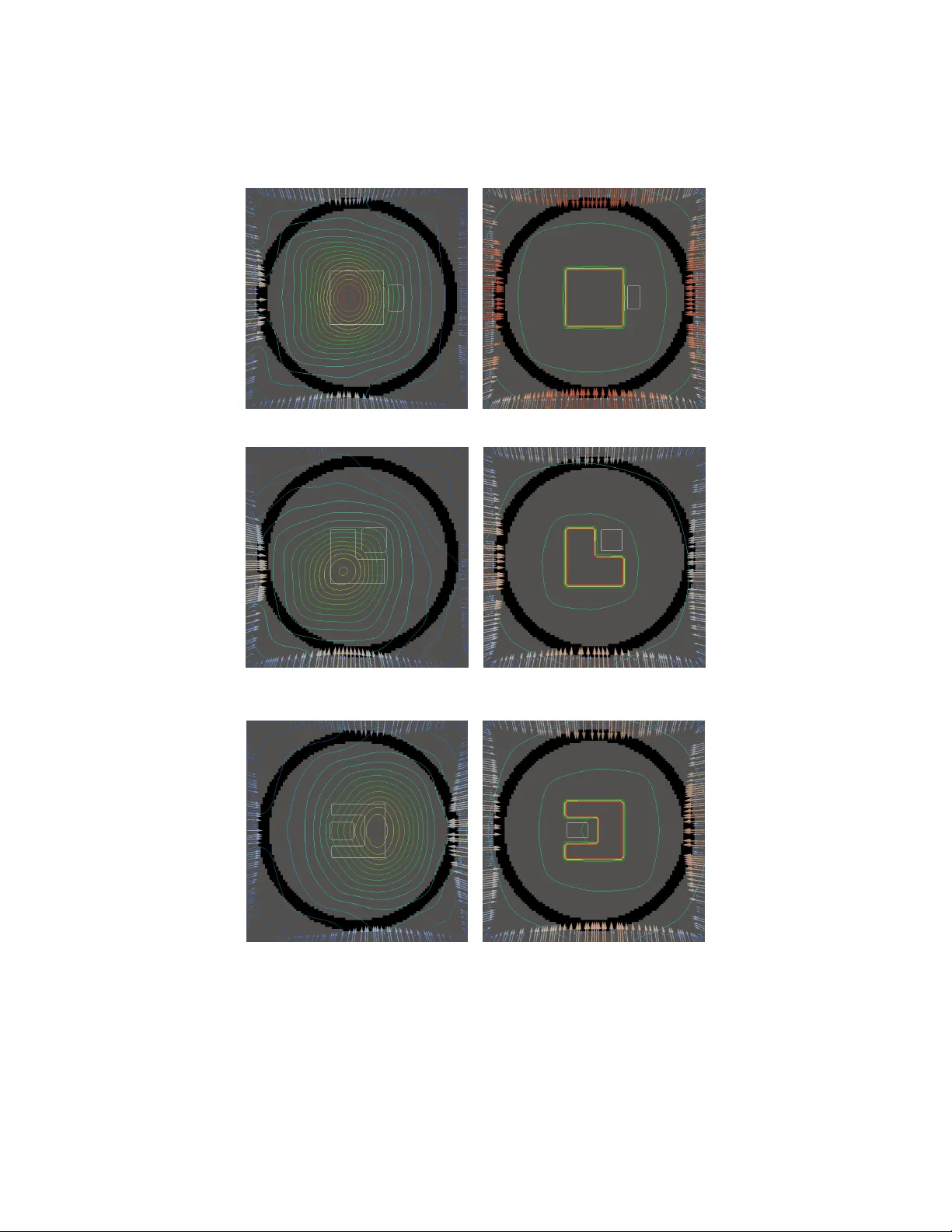
OPTIMAL RADIOTHERAPY TREA TMENT PLANNING USING MINIMUM ENTR OPY MODELS RICHARD BARNARD ∗ , MAR TIN FRANK, MICHAEL HER TY R WTH AACHEN UNIVERSITY, AA CHEN GERMANY Abstract. W e study the problem of finding an optimal radiotherapy treat- ment plan. A time-dep endent Boltzmann particle transp ort mo del is used to model the interaction b et w een radiative particles with tissue. This mo del al- lows for the mo deling of inhomogeneities in the b ody and allo ws for anisotropic sources modeling distributed radiation—as in brach ytherapy—and external beam sources—as in teletherapy . W e study t wo optimization problems: mini- mizing the deviation from a spatially-dep enden t prescribed dose through a qua- dratic trac king functional; and minimizing the surviv al of tumor cells through the use of the linear-quadratic model of radiobiological cell response. F or each problem, we derive the optimalit y systems. In order to solv e the state and ad- joint equations, we use the minimum entrop y approximation; the adv antages of this method are discussed. Numerical results are then presented. 1. Introduction Radiotherap y is one of the main to ols currently in use for the treatment of can- cer. Radiation is dep osited in the tissue with the aim of damaging tumor cells and disrupting their abilit y to repro duce. In this pap er, we are interested in the treat- men t planning problem. W e wish to determine a metho d of delivering a sufficient lev el of radiativ e energy to the tumor cells to ensure cell death. This is balanced b y our our desire to minimize damage to healthy tissue, especially sp ecific critit- cal structures—which we call regions at risk—that should b e damaged as little as p ossible. This problem can b e divided into t w o phases. First, one m ust deter- mine an appropriate external source of radiation that optimally balances these tw o comp eting goals. Secondly , one must devise a means to administer this external source through (in the case of teletherapy) the selection of b eam angles and sim- ilar parameters. W e fo cus on the first of these steps. Once the optimal source is determined, the means of creating such a source would still need to be obtained. Often, the optimal dose will b e determined manually and iterativ ely by an exp e- rienced dosimetrist; this dose consists of selecting several fixed b eam angles and strengths. How ev er, newer metho ds such as Intensit y Mo dulated Radiation Ther- ap y allow for dynamic sources; such a metho d requires more automated algorithms for determining the treatment sc heme [13]. Quan tifying what the “b est” treatment plan is difficult and still unsettled (see [13],[12] for instance). Often a heuristic approach is used b y tec hnicians. Here, w e will study tw o different means of measuring the effectiv eness of a given source. First, we use a general measure: we lo ok to minimize the deviation from a desired ∗ Corresponding author. Email: barnard@mathcces.rwth-aachen.de. 1 2 RICHARD BARNARD ∗ , MAR TIN FRANK, MICHAEL HER TY R WTH AACHEN UNIVERSITY, AACHEN GERMANY distribution of radiation, similar to the ob jective functional used in [13], [2],[10], and [9]. The other metho d we fo cus on in v olv es using radiobiological parameters describing cells’ susceptibilit y to damage from radiation. The cells’ resp onse to the delivered dose is mo deled by the frequently-used linear-quadratic mo del for cell death. A significan t difficulty in using this mo del is that the parameters for cell damage are dep endent on several factors leading to significan t levels of interpatien t heterogeneit y [16],[18],[8],[14]. F urthermore, the parameters can c hange ov er the course of treatment plans as patients exhibit changing levels of radiosensitivity . In particular, [8] studied the optimal treatment planning problem and the dep endence of the optimal dose on different parameters, esp ecially in the face of changing radiosensitivit y . In [14], a method for treatmen t planning that accounts for the uncertain ty in an individual’s sp ecific linear-quadratic parameters was developed. As describ ed in [10], the F ermi-Eyges theory of radiation is used for most dose calculation algorithms; this theory fails to incorp orate prop erly physical in teractions in areas where inhomogeneities such as void-lik e regions o ccur. Here, we will mak e use of a Boltzmann transport model whic h describ es the scattering and absorb- ing effects of the tissue while also allowing for inhomogeneities. Our optimization metho d here differs in tw o significant w ays from that in [10]. First, our mo del is time-dep enden t; we will allow for time-dependent, anisotropic sources which are external (teletherap y) as well as sources distributed in the tissue (brach ytherap y). Second, as opp osed to the spherical harmonics approximation used there, we will mak e use of a minimum entrop y approximation to the Boltzmann transp ort mo del whic h has the b enefit of maintaining sev eral desirable physical prop erties from the original mo del. In Section 2, we will introduce the Boltzmann transp ort model describing the in teractions of the radiation with the tissue and the t wo ob jectiv e functionals whic h w e use to measure the effectiveness of a given dose. In Section 3 we establish optimalit y conditions for b oth ob jectiv e functionals through the adjoint equations of the Boltzmann equation. F rom there, we in tro duce the minim um entrop y ( M 1 ) appro ximation and briefly discuss the adv antages of thi s appro ximation. Numerical results in tw o dimensions are presented for several test cases in Section 5. 2. Ma thema tical Model 2.1. T ransp ort Equation. Let Z ⊂ R 3 b e an open, con v ex, bounded domain with smo oth b oundary and out ward normal n ( x ) , and T > 0 be giv en. The direction of a particle’s mo v ement is Ω ∈ S 2 where S 2 is the 3-dimensional unit sphere. Then we mo del particle transp ort with sources q , q 1 : [0 , T ] × R 3 × S 2 → R by the following equation ψ t ( t, x, Ω) + Ω · ∇ x ψ ( t, x, Ω) + σ t ( x ) ψ ( t, x, Ω) = σ s ( x ) Z S 2 s ( x, Ω · Ω 0 ) ψ ( t, x, Ω 0 ) d Ω 0 (1) + q ( t, x, Ω) with b oundary condition (2) ψ ( t, x, Ω) = q 1 ( t, x, Ω) , ∀ ( t, x, Ω) ∈ Γ − := { ( t, x, Ω) : t ∈ [0 , T ] , x ∈ ∂ Z, n ( x ) · Ω < 0 } and initial condition (3) ψ (0 , x, Ω) = 0 , ∀ ( x, Ω) ∈ Z × S 2 . OPTIMAL RADIOTHERAPY TREA TMENT PLANNING USING MINIMUM ENTROPY MODELS 3 It should b e noted that, (1) do es not explicitly include the energy dep endence of the transp ort of particles. Ho w ev er, as detailed in [9], the Boltzmann Contin uous Slo wing Down mo del, whic h do es include energy dependence, can b e transformed in to a problem suc h as (1) where the initial-v alue condition in tuitiv ely describes the ph ysically reasonable condition that no particles are of “infinite” energy . In general, the term q denotes a distributed radiative source which w ould b e appropriate for applications in brach ytherap y; m ean while, q 1 seems a natural means of mo deling the effects of external b eams in teletherapy applications. How ev er, as describ ed in Section 4, the role of the con trol on the incoming b oundary is difficult to mo del in the context of the M 1 appro ximation (along with similar moment approximations) to (1). With this in mind, throughout this pap er we will assume q 1 ≡ 0; that is, we will replace (2) with the incoming b oundary condition (4) ψ ( t, x, Ω) = 0 , ∀ ( t, x, Ω) ∈ Γ − . W e will address in Section4 a means of mo deling the case of teletherapy using the distributed control. The quantit y ψ ( t, x, Ω) cos θdAd Ω is in terpreted as the n umber of particles at time t passing through dA at x in the direction d Ω near Ω where θ is the angle b etw een Ω and dA. The total cross-section σ t ( x ) is the sum of the absorption cross-section σ a ( x ) and scattering cross-section σ s ( x ) . Finally , the scattering kernel—in tuitiv ely describing the probability of a particle changing direction from Ω 0 to Ω at x ∈ Z after a scattering ev ent—is normalized; that is, it satisfies for all x, Z 1 − 1 s ( x, η ) dη = 1 2 π . In this paper, w e will usethe simplified Hen yey-Greenstein kernel (see [1] for more) s H G ( x, η ) := 1 − g ( x ) 2 4 π (1 + g ( x ) 2 − 2 g ( x ) η ) 3 / 2 where g is the av erage cosine of the scattering angle. F ollowing [10], we define the op erators ( A ψ )( t, x, Ω) = − ψ t ( t, x, Ω) − Ω · ∇ x ψ ( t, x, Ω) ( K ψ )( t, x, Ω) = σ s ( x ) Z S 2 s ( x, Ω 0 · Ω) ψ ( t.x, Ω 0 ) d Ω 0 (Σ ψ )( t, x, Ω) = σ t ( x ) ψ ( t, x, Ω) and make the following general assumptions: (H-1) σ t , σ s , s ≥ 0 , (H-2) σ t , σ s ∈ L ∞ ( Z ) , (H-3) σ t ( x ) − σ s ( x ) ≥ α > 0 , ∀ x ∈ Z . W e note that (H-1) and (H-2) are reasonable physically and that as long as the medium under consideration is absorbing, the co ercivit y h yp othesis (H-3) is satisfied. These assumptions imply that the op erators K , Σ : L 2 ([0 , T ] × Z × S 2 ) → L 2 ([0 , T ] × Z × S 2 ) are b ounded and linear op erators. Finally , we note that if we define D ( A ) = { ψ ∈ L 2 ([0 , T ] × Z × S 2 ) : ψ t , Ω · ∇ x ψ ∈ L 2 ([0 , T ] × Z × S 2 ) } , 4 RICHARD BARNARD ∗ , MAR TIN FRANK, MICHAEL HER TY R WTH AACHEN UNIVERSITY, AACHEN GERMANY then A : D ( A ) → L 2 ([0 , T ] × Z × S 2 ) is a well-defined linear op erator. W e also let ^ D ( A ) denote the set of functions of D ( A ) which also satisfy (4) and (3), for q 1 ≡ 0 . Then w e can conclude—for instance, b y Ch. XXI, 2, Theorem 3 of [5] the following holds. Theorem 2.1. Supp ose that (H-1)-(H-3) hold and that q 1 ∈ L 2 ([0 , T ] × Z × S 2 ) is nonne gative. Then (1) has a unique solution ψ ⊂ ˜ D ( A ) . W e define the control-to-state mapping E : L 2 ([0 , T ] × Z × S 2 ) → D ( A ) as the map which maps a source q to the corresp onding solution ψ to − A ψ + Σ ψ = K ψ + q sub ject to (4) and (3). By the ab o v e, this is a well-defined, linear op erator. As in [10], it is also b ounded. Prop osition 2.1. L et h· , ·i 2 denote the standar d inner pr o duct on L 2 ([0 , T ] × Z × S 2 ) . Then it holds that, for ψ satisfying (4) and (3), h− A ψ + Σ ψ − K ψ , ψ i 2 ≥ α || ψ || 2 2 and thus E is a b ounde d op er ator. Pr o of. W e note that, by an argumen t analogous to the pro of of Lemma 3.1 of [10], h Σ ψ − K ψ , ψ i 2 ≥ α || ψ || 2 2 . Additionally , by in tegration by parts and the initial and b oundary conditions, h− A ψ , ψ i 2 = Z [0 ,T ] × Z × S 2 ( ψ t ψ ) dtdxd Ω + Z [0 ,T ] × Z × S 2 (Ω · ∇ x ψ ) ψ dtdxd Ω = Z Z × S 2 1 2 ψ 2 ( T , x, Ω) dxd Ω + Z [0 ,T ] Z Z div  Z S 2 1 2 Ω ψ 2 d Ω  dxdt = Z Z × S 2 1 2 ψ 2 ( T , x, Ω) dxd Ω + Z [0 ,T ] Z ∂ Z × S 2 1 2 (Ω · n ( x )) + ψ 2 dxd Ω dt ≥ 0 . Com bining the tw o inequalities gives the desired result.  2.2. Ob jective F unctionals. W e consider tw o ob jective functionals. In eac h case, w e neglect the incoming b oundary source term by fixing q 1 ≡ 0 for reasons which are discussed in 4. Also, we are primarily interested only in the total dose dep osited as a function of x , which w e denote b y the operator D : L 2 ([0 , T ] × Z × S 2 ) → L 2 ( Z ) whic h is defined as D ψ ( x ) := Z [0 ,T ] × S 2 ψ ( t, x, Ω) dtd Ω . The first functional is a quadratic tracking which measures the deviation from a prescrib ed dose D ( x ) (5) J T ( ψ , q ) := Z Z c 1 ( D ψ − D ) 2 dx + Z Z c 2 D ( q ) 2 dx. OPTIMAL RADIOTHERAPY TREA TMENT PLANNING USING MINIMUM ENTROPY MODELS 5 Here c 1 , c 2 > 0 are spatially dep enden t weigh ting functions. One such weigh ting function, used in [10], for c 1 is c 1 = c T χ Z T + c R χ Z R + c N χ Z N , where c T , c R , c N are constants and Z T , Z R , Z N are, resp ectively , the p ortions of Z corresp onding to the tumor, a region at risk, and normal tissue with Z = Z T ∪ Z R ∪ Z N . This functional differs sligh tly from that studied in [10] in that w e are concerned with the dose dep osited but the source is allow ed to b e angle-dep enden t. In that w ork, the ob jective functional studied for anisotropic con trols also assumed a desired anisotropic distribution was to b e track ed, as opp osed to simply a total dose. Though this ob jectiv e functional does not attempt to mo del cell resp onse to the dose, it do es hav e the b enefits of not requiring as inputs the radiobiological parameters needed for such a mo del. The second ob jectiv e functional inv olv es mo deling cell death as a function of D ( ψ ). W e will use the linear-quadratic model ([14]), neglecting cell gro wth and repair rates. In a reference volume for a giv en dose D , the fraction of surviving cells of a single t yp e is given b y (6) S F = exp( − αD − β D 2 ) where α, β are parameters dep enden t the type of cell b eing irradiated. This mo del has b een used extensively for determining dose strategies (for instance, [4, 16, 15, 18, 11] and, in a mo dified form, [8]). The surviving fraction is often used to determine the tumor control probability for a given region: T C P = exp Z  − ρ exp( − α i D i − β i D 2 i )  where ρ is the densit y of tumor cells as a function of space. W e consider a contin uous measure of the num ber of surviving cells of the v arious cell types in Z. W e consider a single type of tumor cell and assign this cell t yp e the index 0. The remaining cell types are giv en index i = 1 , . . . , N . Then, for cell densities ρ i ( x ) ≥ 0 with P N i =0 ρ i ( x ) = 1 , we define J S F ( ψ , q ) := a 0 Z Z ρ 0 exp  − α 0 D ψ − β 0 ( D ψ ) 2  (7) + N X i =1 a i Z Z ρ i  1 − exp  − α i D ψ − β i ( D ψ ) 2   + c 2 2 Z Z ( D q ) 2 where we assign constant w eigh ts for each cell type a i > 0 and the con trol c 2 > 0 . F or either cost functional, w e set U ( x ) ≥ 0 to be the maxim um allo wed source at x ∈ Z. Let L 2 ad ([0 , T ] × Z × S 2 ) denote the set of admissible con trols–that is, those controls satisfying q ≥ 0 and Z S 2 q ( t, x, Ω) d Ω ≤ U ( x ) almost ev erywhere. Note that this subset of L 2 ([0 , T ] × Z × S 2 ) is nonempt y , closed, and conv ex. 6 RICHARD BARNARD ∗ , MAR TIN FRANK, MICHAEL HER TY R WTH AACHEN UNIVERSITY, AACHEN GERMANY 3. Optimality conditions W e are, then, in terested in tw o separate optimal control problems: the mini- mization of tracking error ( P T ) min ψ ∈ ^ D ( A ) ,q ∈ L 2 ad [0 ,T ] × Z × S 2 ) J T ( ψ , q ) , s.t. E ( q ) = ψ . and the minimization of tumor cell surviving fraction balanced against normal cell death ( P S F ) min ψ ∈ ^ D ( A ) ,q ∈ L 2 ad ([0 ,T ] × Z × S 2 ) J S F ( ψ , q ) , s.t. E ( q ) = ψ . In order to obtain optimality conditions for P T and P S F , w e follow the example of [17]. One of the adv antages of using J T as the ob jective functional is the following: Theorem 3.1. Given (H-1)-(H-3), and ψ ∈ ^ D ( A ) with D = D ( ψ ) and c 1 , c 2 > 0 , then P T has a unique solution q ∗ ∈ L 2 ad ([0 , T ] × Z × S 2 ) . Pr o of. W e note that the reduced ob jective functional j T ( q ) = J T ( E ( q ) , q ) is a con- v ex functional ov er the closed,conv ex set L 2 ad ([0 , T ] × Z × S 2 ) of the Hilb ert space L 2 ([0 , T ] × Z × S 2 ) and that E is linear and b ounded. By Theorem 2.16 of [17], there exists a unique minimizer for problem P T .  W e no w turn to the existence of an optimal control for P S F . Because the asso- ciated reduced ob jective functional is nonconv ex, we can not assume existence of a unique optimal control. Theorem 3.2. Given (H-1)-(H-3) and c i , a > 0 ther e exists at le ast one optimal c ontr ol q ∗ ∈ L 2 ad ([0 , T ] × Z × S 2 ) for P S F . Pr o of. W e note that J S F is conv ex with resp ect to q and that the set of admissible con trols is closed, conv ex, and b ounded. This, coupled with the b oundedness of the op erator E allo ws us to conclude that the infimum of J S F o ver L 2 ad ([0 , T ] × Z × S 2 ) is finite and that any weakly conv ergen t minimizing sequence of controls q n will con verge to an admissible control q ∗ . By the linearity of A , Σ , K , w e conclude that the corresp onding solutions conv erge strongly to a solution corresp onding to the q ∗ . (see Theorem 5.7 of [17]). The con vexit y of J S F as a functional of q allows us to conclude this control is optimal, as in Theorem 4.15 of [17].  W e next note the following from [5]: Prop osition 3.1. Under (H-1)-(H-3), for any r ∈ L 2 ([0 , T ] × Z × S 2 ) , A λ + Σ λ − K λ = r λ = 0 on Γ + λ ( T , x, Ω) = 0 , ∀ ( x, Ω) ∈ Z × S 2 . has a unique solution λ ∈ L 2 ([0 , T ] × Z × S 2 ) , and the solution op er ator E ∗ is line ar, b ounde d, and the adjoint to E . No w, we are ready to turn to the optimality conditions for P T , which is similar to that found in [10]. OPTIMAL RADIOTHERAPY TREA TMENT PLANNING USING MINIMUM ENTROPY MODELS 7 Theorem 3.3. F or a desir e d distribution D ∈ L 2 ( Z ) and under the assumptions (H-1)-(H-3), q ∗ ∈ L 2 ad ([0 , T ] × Z × S 2 ) is the unique optimal solution to P T if and only if (8) q ∗ ( t, x, Ω) = pro j [0 ,U ( x )]  − 1 c 2 ( x ) λ ∗ ( t, x, Ω)  wher e λ ∗ = E ∗ ( c 1 ( D ( ψ ∗ ) − D )) , ψ ∗ = E ( q ∗ ) , and pro j S ( · ) denotes pr oje ction onto the close d set S. Pr o of. The gradient of j T is c 1 E ∗ ( D E ( q ∗ ) − D )) + c 2 D q and so we conclude, using the same arguments of Theorem 2.25, Lemma 2.26, and Theorem 2.27 of [17].  This means that the optimalit y system for P T is (9)      − A ψ ∗ + Σ ψ ∗ = K ψ ∗ + q ∗ , A λ ∗ + Σ λ ∗ = K λ ∗ + c 1 D ( E ( q ∗ ) − D ) , q ∗ = pro j [0 ,U ( x )] ( − 1 c 2 λ ∗ ) with ψ ∗ satisfying (4) and (3), λ ∗ = 0 on Γ + , and λ ( T , x, Ω) = 0 on Z × S 2 . The necessary condition for the optimality of a source for P S F is of a similar form. Theorem 3.4. F or a given distribution of c el ls ρ i , i = 0 , 1 , . . . N and the asso ciate d line ar-quadr atic c el l de ath p ar ameters α i , β i > 0 , a lo c al ly optimal q ∗ ∈ L 2 ad ([0 , T ] × Z × S 2 ) for J S F must b e such that (10) q ∗ ( t, x, Ω) = pro j [0 ,U ( x )]  − 1 c 2 ( x ) λ ∗ ( t, x, Ω)  wher e λ ∗ = E ∗ ( r ∗ ) for r ∗ = h  − α 0 − 2 β 0 D ψ ∗  c 0 ρ 0 exp[ − α 0 D ψ ∗ − β 0 ( D ψ ∗ ) 2 ]  i − N X i =1 h  − α i − 2 β i D ψ ∗  c i ρ i exp[ − α i D ψ ∗ − β i ( D ψ ∗ ) 2 ]  i and ψ ∗ = E ( q ∗ ) . Pr o of. The reduced cost functional j S F ( q ) = J S F ( E ( q ) , q ) is F r ´ ec het differentiable due to the differen tiabilit y of the in tegrands in J S F and the linearit y and con tin uit y of E . F or simplicity , we assume ρ 0 ≡ 1 (and thus ρ i ≡ 0 for i ≥ 1) first. W e then get that for a lo cally optimal q ∗ and any other admissible control q , j 0 S F ( q ∗ )( q − q ∗ ) ≥ 0 where, by the linearity of the adjoint solution op erator E ∗ and the chain rule, j 0 S F ( q ∗ )( q − q ∗ ) = c 0 Z Z  − α 0 − 2 β 0 D E ( q ∗ )  c 0 ρ 0 exp[ − α 0 D E ( q ∗ ) − β 0 ( D E ( q ∗ )) 2 ]  E ( q − q ∗ ) + c 2 Z Z q ∗ ( q − q ∗ ) = Z Z E ∗ (( − α 0 − 2 β 0 D E ( q ∗ )  c 0 ρ 0 exp[ − α 0 D E ( q ∗ ) − β 0 ( D E ( q ∗ )) 2 ]  ( q − q ∗ ) + c 2 Z Z q ∗ ( q − q ∗ ) . 8 RICHARD BARNARD ∗ , MAR TIN FRANK, MICHAEL HER TY R WTH AACHEN UNIVERSITY, AACHEN GERMANY This leads to the minimum principle (by an argumen t analogous to that found on pages 68-70 of [17]), whic h states that min q ∈ L 2 ad ([0 ,T ] × Z × S 2 ) [( λ ∗ + c 2 q ∗ ) q ] is attained almost everywhere at q ∗ whic h leads us to conclude that q ∗ satisfies (10). Now if we drop the assumption that ρ i ≡ 1 , and allow for the presence of other sp ecies, the argument follows through in a nearly iden tical fashion.  This gives the necessary optimality system (11)      − A ψ ∗ + Σ ψ ∗ = K ψ ∗ + q ∗ , A λ ∗ + Σ λ ∗ = K λ ∗ + r ∗ , q ∗ = pro j [0 ,U ( x )] ( − 1 c 2 λ ∗ ) where r ∗ is as in Theorem 3.4. 4. Minimum entropy closure F or our purp oses, solving (1) in full is unnecessary . W e note that b oth J T and J S F do not need the exact photon densities as functions of the angular v ariable; it w ould b e enough to determine the zeroth moment, which is the total energy at a giv en ( t, x ): ψ (0) ( t, x ) = Z S 2 ψ ( t, x, Ω) d Ω . In light of this, we av erage (1) ov er the angular v ariable and obtain (12) ∂ t ψ (0) ( t, x ) + ∇ x · ψ (1) ( t, x ) + σ t ( x ) ψ (0) ( t, x ) = σ s ( x ) ψ (0) ( t, x ) + q (0) ( t, x ) where ψ (1) ( t, x ) = Z S 2 Ω ψ ( t, x, Ω) d Ω is the first momen t, or the flux v ector and q (0) is the a v erage of q ov er all directions. By multiplying (1) by Ω and taking the av erage ov er all directions, w e get (13) ∂ t ψ (1) ( t, x ) + ∇ x · ψ (2) ( t, x ) + σ t ( x ) ψ (1) ( t, x ) = σ s ( x ) g ψ (1) ( t, x ) + q (1) ( t, x ) where ψ (2) ( t, x ) = Z S 2 (Ω ⊗ Ω) ψ ( t, x, Ω) d Ω is the second momen t, or the pressure tensor of the radiation field, and q (1) is the first momen t of the control. W e note that if we contin ued this process of multiplying (1) by monomials of Ω and integrating ov er S 2 , we would alwa ys ha ve an equation relating the n th momen t to the ( n + 1) th momen t. If w e w ant a closed system, then, w e must select an approximation to the ( n + 1) th momen t ψ ( n +1) = D ( ψ (0) , . . . , ψ ( n ) ) . Here, we consider the minimum entrop y closure ( M 1 ) to approximate ψ (2) . This in volv es searching for I which minimizes H ∗ R ( I ) = Z S 2 h ∗ R ( I ) d Ω where h ∗ R ( I ) = 2 k ν 2 ( n log n − ( n + 1) log( n + 1)) , with n = I 2 hν 3 , OPTIMAL RADIOTHERAPY TREA TMENT PLANNING USING MINIMUM ENTROPY MODELS 9 and k is the Boltzmann constant, h is the Planck constant, and ν is the frequency of the radiation. W e constrain the entrop y minimization by requiring, naturally , that Z S 2 I d Ω = ψ (0) , and Z S 2 Ω I d Ω = ψ (1) . in [6], the entrop y minimizer was obtained explicitly by setting ψ (2) = D ( f ) E where the relative flux is f = ψ (1) /ψ (0) , the Eddington tensor D , is D ( f ) = 1 − χ ( f ) 2 I + 3 χ ( f ) − 1 2 f ⊗ f | f | 2 and the Eddington factor χ is χ ( f ) = 1 3 (5 − 2 p 4 − 3 | f | 2 ) . This c hoice of the Eddington factor preserv es sev eral reasonable ph ysical properties. Imp ortan tly , the flux is limited; that is, | f | < 1 . This preserv es the finite b ound the sp eed that information trav els through the system. Also, the distribution is nonnegativ e, which we would like to ensure. W e note that neither prop ert y is sat- isfied for sev eral common closure choices which use a diffusion approximation, such as the spherical harmonics metho d(also known as P N metho ds) [3]. In [7], the M 1 appro ximation w as seen via numerical tests to provide a high quality approximation when compared with Monte Carlo-based metho ds. Despite these adv antages, the M 1 do es hav e several drawbac ks. Due to the non- linearit y of the M 1 appro ximation (as opp osed to the P N appro ximation [10]), we can not exp ect that the systems obtained by applying the M 1 appro ximation to the optimality systems will match the optimality systems obtained by optimizing the M 1 appro ximation to (1). Also, as mentioned briefly ab o v e, the use of moment mo dels complicates the incorp oration of b oundary conditions. The b oundary con- dition (4) describ es only the incoming particles, whereas boundary conditions for (12) and (13) require us to prescrib e v alues for the full moments. In light of this, w e use U ( x ) to approximate b oundary control by setting it as U ( x ) = ( q max , if d ∂ Z ( x ) ≤  δ otherwise , where q max > 0 is a total maximum source level, , δ > 0 are sufficien tly small parameters, and d ∂ Z denotes the usual distance from the b oundary of Z . W e note that the first tw o equations in b oth (9) and (11) are v ery similar and w e thus use the M 1 closure to solve the state and adjoint equations. That is, w e take an optimize- then-discretize approach to P T and P S F as opp osed to a discretize-then-optimize approac h. 5. 2-D Numerical Tests In this section, w e study the 2-dimensional region Z := [ − 1 , 1] × [ − 1 , 1] . W e define a void-lik e region Z V := { 0 . 8 ≤ | x | ≤ 0 . 9 } On Z V , the scattering and absorbtion cross-sections σ s , σ a ha ve v alues that differ from those elsewhere; these are summarized in T able 1 for the sp ecific v alues. 10 RICHARD BARNARD ∗ , MAR TIN FRANK, MICHAEL HER TY R WTH AACHEN UNIVERSITY, AACHEN GERMANY Z V Z \ Z V σ a 0.001 0.05 σ s 0.01 0.5 T able 1. Material parameters for P S F Z T Z R Z N α 0.52 0.170 0.170 β 0.171 0.0078 0.0078 T able 2. Cell-resp onse parameters for P S F Z T Z R Basic T arget [ − 0 . 25 , 0 . 25] × [ − 0 . 25 , 0 . 25] [ . 254 , 0 . 379] × [ − 0 . 125 , 0 . 125] In termediate T arget ([ − 0 . 25 , 0 . 25] × [ − 0 . 25 , 0]) [0 . 04 , 0 . 25] × [0 . 04 , 0 . 25] ∪ ([ − 0 . 25 , 0] × [0 , 0 . 25]) Complex T arget ([ − 0 . 25 , 0 . 25] × [ − 0 . 25 , − 0 . 125]) [ − 0 . 25 , − 0 . 04] × [ − 0 . 121 , 0 . 121] ∪ ([ − 0 . 25 , 0 . 25] × [0 . 125 , 0 . 25]) ∪ ([0 . 04 , 0 . 25] × [ − 0 . 125 , 0 . 125]) T able 3. Lo cations of T umor and Risk Region The final parameter of the ph ysical medium to be defined is the scattering phase function. F or simplicity in our test problem, we define g ≡ 0 . 85 . Other, more in volv ed, kernels might b e used in this range for g to agree with Mie scattering theory as in [1]. F or testing, w e use three tumor/risk region regions similar to those in [13]. Specif- ically , w e define the regions in T able 3 and are shown in Figure 1; the void region is shown in black and the tumor and risk regions are traced in white. In the basic target case, seen in Figure 1(a), the tumor region is a box, as is the risk region. The second, intermediate target case, seen in Figure 1(b), inv olv es an L-shap ed tumor around a b ox-shaped risk region. Finally , the complex target case in Figure 1(c) in volv es a C-shap ed tumor around a risk region. W e will solve b oth P T and P S F for eac h geometry seen in Figure 1. F or P T for eac h example, we set D ≡ T on Z T and 0 elsewhere, corresp onding to an av erage (ov er time) dose of 1 , and c 1 = c T χ Z T + c R χ Z R + c N χ Z N with c T = 25 , c R = 150 , c N = 1 . F or P S F , we set ρ 0 ≡ χ Z T , ρ 1 ≡ χ Z R , ρ 2 ≡ χ Z N , with w eigh ts a 0 = 500 , a 1 = 2000 , a 2 = 1 . The LQ parameters are shown b elo w; the tumor region uses parameters for Lewis Lung tumor cells and the risk region and normal region use parameters for V79 (normal Chinese hamster lung tissue); b oth sets of parameters are taken from [16]. W e use a simple gradien t descen t algorithm to determine an optimal control for each of the three targets and for each ob jective functional. The M 1 appro ximations to b oth the state and adjoin t equations are solv ed with a finite volume solv er using approximately 10,000 cells with final time T = 5 . The parameters δ and  in the definition of U ( x ) are chosen as min { ∆ x, ∆ y } (10 − 4 ) t and min { ∆ x, ∆ y } , resp ectiv ely , where ∆ x, ∆ y OPTIMAL RADIOTHERAPY TREA TMENT PLANNING USING MINIMUM ENTROPY MODELS 11 (a) Basic T arget (b) Intermediate T arget (c) Complex T arget Figure 1. Example cases are the mesh sizes. W e consider the algorithm as conv erged if b oth the difference b et w een consecutive iterates and || j 0 ( q ) || ∞ are smaller than 10 − 4 . Figure 2 shows the optimal b oundary source term for b oth P T and P S F . The v ectors shown on the b oundary are the time-integrated v alues of q (1) normalized and then scaled by q (0) . In Figures 2(a), 2(c), and 2(e) (corresp onding to P T ), the isolines are spaced at 5% in terv als of the maximum of the desired dose (here, 5). In the intermediate and trac king cases, w e see that relatively lo w dose levels are attained, primarily due to the high penalty to an y dose deposited in the risk region. In Figures 2(b), 2(d), and 2(f )(corresp onding to P S F ), the isolines are spaced at in terv als of 10% of cells killed. Here a high prop ortion of the tumor cells are killed (in each case 80% − 90%) while in the Intermediate and Basic cases, the tumor has at least 60% surviv al; in the Complex case, the risk region has 50% − 60% surviv al. The dose deposited in P T c hanges significan tly when w e alter the relativ e weigh ts c T and c R . In Figure ?? , we see the results for solving P T , and P S F where w e set c R = 50 and a 1 = 1000 (all other parameters are unchanged). In b oth the basic and intermediate cases, the dose delivered to the tumor is significantly higher while also remaining largely concentrated on the tumor. This is slightly less true in the 12 RICHARD BARNARD ∗ , MAR TIN FRANK, MICHAEL HER TY R WTH AACHEN UNIVERSITY, AACHEN GERMANY (a) T racking, Basic T arget (b) Surviving F raction, Basic T arget (c) T racking, In termediate T arget (d) Surviving F raction, Intermediate T arget (e) T racking, Complex T arget (f ) Surviving F raction, Complex T arget Figure 2. Optimal b oundary source for P T , in (a),(c),(e) and P S F in (b),(d),(f ) OPTIMAL RADIOTHERAPY TREA TMENT PLANNING USING MINIMUM ENTROPY MODELS 13 complex case. In the figures for P S F , there is no general change in the pattern of cell death, ho wev er the risk region in the first tw o cases has 50% cell surviv al whereas the complex case has approximately 40% − 50% cell surviv al. How ev er, this lack of c hange in pattern can partially b e attributed to the tumor cells b eing more susceptible to the radiation dose. W e conclude with a final set of n umerical examples whic h restrict the lo cation of the source b y altering the definition of U ( x ) . Here we require that q ≤ δ on one side of the b oundary . F or the basic and intermediate case, we require that the external source not come from the left side of Z. F or the complex case, w e disallo w sources on the right side (as the optimal source is nearly zero on the right side in the complex case for P T ). Figure 4 shows the optimal solution for b oth problems, using the same p enalization parameters used in Figure 2. The optimal dose for P T is significan tly w orse, with the tumor in the in termediate and complex cases getting a dose b elo w 3 . Ho wev er, the tumor cells hav e a surviv al of 10% or less for eac h case and the risk region has a surviv al rate of 60% or higher in each case. Clearly , the choice of relative weigh ts c T , c R and a i affects the optimal solution. Ho wev er, w e hav e curren tly no systematic a priori metho d of selecting the relative w eights in either problem. Suc h a metho d should take into account the relativ e imp ortance of the different tissues and the susceptibilities of the v arious cell types, leading to a p ossibly nonin tuitiv e scheme. Without such a metho d, sev eral opti- mization runs may b e required to find an appropriate treatment strategy . W e also note that the optimization do es not consider the feasibility of the optimal source. In fact, the optimal b oundary con trol in all of the numerical results are spread out along the b oundary , as opp osed to b eing fo cused in a b eam configuration. F urther mo deling w ould b e required in order for the cost function to penalize non-b eam like configurations. A cknowledgments This work has b een supp orted by HE5386/8-1, FR 2841/1-1 and the Seedfunds of R WTH Aachen. References [1] E. D. A ydin, C. R. E. de Oliveira, and A. J. H. Goddard , A c omp arison b etwe en tr ans- p ort and diffusion calculations using a finite element-spheric al harmonics r adiation tr ansport metho d , Medical Ph ysics, 29 (2002), pp. 2013–2023. [2] C. B ¨ orgers , The r adiation ther apy planning pr oblem , in Computational radiology and imag- ing (Minneap olis, MN, 1997), v ol. 110 of IMA V ol. Math. Appl., Springer, New Y ork, 1999, pp. 1–16. [3] T. Brunner , F orms of appr oximate r adiation tr ansp ort , Sandia Report, (2002). [4] R. G. Dale , The applic ation of the line ar-quadr atic dose-effe ct e quation to fractionate d and pr otracte d r adiotherapy , Br J Radiol, 58 (1985), pp. 515–528. [5] R. D autra y and J.-L. Lions , Mathematic al analysis and numeric al metho ds for science and te chnology. , vol. 6, Springer-V erlag, Berlin, 1993. [6] B. Dubroca and J.-L. Feugeas , ´ Etude th´ eorique et num´ erique d’une hi´ er archie de mo d` eles aux moments p out le transfert r adiatif , Analyse n um´ erique, 329 (1999), pp. 915–920. [7] R. Duclous, B. Dubroca, and M. Frank , A deterministic p artial differential e quation mo del for dose c alculation in ele ctr on r adiotherapy , Physics in Medicine and Biology , 55 (2010), p. 3843. [8] B. C. Ferreira, P. Ma vroidis, M. Adamus-G ´ orka, R. Svensson, and B. K. Lind , The imp act of differ ent dose-r esp onse par ameters on biologic al ly optimize d imrt in bre ast c anc er , Physics in Medicine and Biology , 53 (2008), p. 2733. 14 RICHARD BARNARD ∗ , MAR TIN FRANK, MICHAEL HER TY R WTH AACHEN UNIVERSITY, AACHEN GERMANY (a) T racking, Basic T arget (b) Surviving F raction, Basic T arget (c) T racking, In termediate T arget (d) Surviving F raction, Intermediate T arget (e) T racking, Complex T arget (f ) Surviving F raction, Complex T arget Figure 3. Optimal results with low er p enalty to dose in Z R OPTIMAL RADIOTHERAPY TREA TMENT PLANNING USING MINIMUM ENTROPY MODELS 15 (a) T racking, Basic T arget (b) Surviving F raction, Basic T arget (c) T racking, In termediate T arget (d) Surviving F raction, Intermediate T arget (e) T racking, Complex T arget (f ) Surviving F raction, Complex T arget Figure 4. Optimal results with one edge blo c k ed 16 RICHARD BARNARD ∗ , MAR TIN FRANK, MICHAEL HER TY R WTH AACHEN UNIVERSITY, AACHEN GERMANY [9] M. Frank, M. Her ty, and A. N. Sandjo , Optimal r adiother apy tr e atment planning governe d by kinetic e quations , Math. Mo dels Metho ds Appl. Sci., 20 (2010), pp. 661–678. [10] M. Frank, M. Her ty, and M. Sch ¨ afer , Optimal tr e atment planning in radiother apy b ase d on Boltzmann tr ansport c alculations , Math. Models Metho ds Appl. Sci., 18 (2008), pp. 573– 592. [11] C. R. King, T. A. DiPetrillo, and D. E. W azer , Optimal r adiother apy for pr ostate c an- c er: pr e dictions for c onventional external b eam, imrt, and br achyther apy fr om r adiobiolo gic mo dels , International Journal of Radiation Oncology*Biology*Ph ysics, 46 (2000), pp. 165 – 172. [12] K.-H. K ¨ ufer, M. Monz, A. Scherrer, P. S ¨ uss, F. Alonso, A. S. A. Sul t an, T. Bor tfeld, and C. Thieke , Multicriteria optimizaton in intensity mo dulate d r adiother apy planning , in Handbo ok of optimization in medicine, vol. 26 of Springer Optim. Appl., Springer, New Y ork, 2009, pp. 123–167. [13] D. M. Shep ard, M. C. Ferris, G. H. Olivera, and T. R. Mackie , Optimizing the delivery of radiation ther apy to c anc er p atients , SIAM Review, 41 (1999), pp. 721–744. [14] C. P. South, M. P ar tridge, and P. M. Ev ans , A theor etic al fr amework for pr escribing r adiotherapy dose distributions using patient-sp e cific biolo gical information , Medical Physics, 35 (2008), pp. 4599–4611. [15] G. G. Steel, J. M. Deacon, G. M. Duchesne, A. Hor wich, L. R. Kelland, and J. H. Peacock , The dose-rate effe ct in human tumour c el ls , Radiotherapy and Oncology , 9 (1987), pp. 299 – 310. [16] G. G. Steel, J. D. Down, J. H. Peacock, and T. C. Stephens , Dose-rate effe cts and the r epair of r adiation damage , Radiotherapy and Oncology , 5 (1986), pp. 321 – 331. [17] F. Tr ¨ ol tzsch , Optimal contr ol of p artial differ ential equations: the ory, metho ds, and ap- plic ations , vol. v. 112 of Graduate studies in mathematics, American Mathematical Society , Providence, R.I., 2010. [18] S. Webb , Optimum p arameters in a mo del for tumour c ontrol pr obability including interpa- tient hetero geneity , Physics in Medicine and Biology , 39 (1994), pp. 1895–1914.