Reduced models of networks of coupled enzymatic reactions

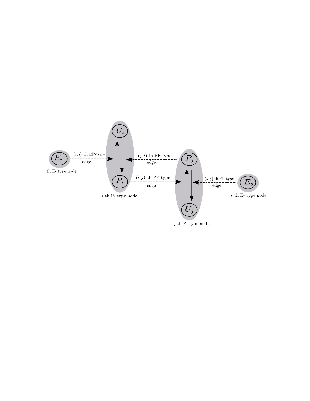
Reduced mo dels of net w orks of coupled enzymatic reactions Ajit Kumar a , Kre ˇ simir Josi ´ c a,b, ∗ a Dep artment of Mathematics, University of Houston, Houston TX 77204-3008, USA b Dep artment of Biolo gy and Bio chemistry, University of Houston, Houston TX 77204-5001, USA Abstract The Mic haelis-Menten equation has pla y ed a cen tral role in our understanding of bio c hemical pro cesses. It has long b een understo o d how this equation approximates the dynamics of irrev ersible enzymatic reactions. Ho wev er, a similar appro ximation in the case of net w orks, where the pro duct of one reaction can act as an enzyme in another, has not b een fully dev elop ed. Here we rigorously deriv e such an approximation in a class of coupled enzymatic net works where the individual in teractions are of Michaelis-Men ten t yp e. W e show that the sufficien t conditions for the v alidit y of the total quasi ste ady state assumption (tQSSA) , obtained in a single protein case b y Borghans, de Boer and Segel can b e extended to sufficien t conditions for the v alidit y of the tQSSA in a large class of enzymatic net works. Secondly , we deriv e reduced equations that approximate the netw ork’s dynamics and in volv e only protein concen trations. This significantly reduces the n umber of equations necessary to mo del such systems. W e pro v e the v alidit y of this appro ximation using geometric singular p erturbation theory and results ab out matrix differen tiation. The ideas used in deriving the appro ximating equations are quite general, and can b e used to systematize other model reductions. Keywor ds: Mic haelis Menten, quasi steady state, total quasi steady state, protein in teraction netw orks, coupled enzymatic net works, geometric singular p erturbation 1. In tro duction The Michaelis-Men ten (MM) scheme [3, 20] is a fundamen tal building blo c k of many mo dels of protein interactions: An enzyme, E , reacts with a protein, X , resulting in an in termediate complex, C . In turn, this complex can break do wn into a pro duct, X p , and the enzyme E . It is frequently assumed that formation of C is reversible while its breakup is not. The pro cess is represen ted b y the following sequence of reactions [3, 20, 21] X + E k 1  k − 1 C k 2 → X p + E . (1.1) F requen tly catalytic activity in protein interaction net work is mo deled b y MM equa- tions [14, 24, 33, 32, 6, 4, 25, 9]. This gives rise to c ouple d enzymatic networks , where the ∗ Corresp onding author Email addr esses: ajitkmar@math.uh.edu (Ajit Kumar), josic@math.uh.edu (Kre ˇ simir Josi ´ c) Pr eprint submitte d to Journal of The or etic al Biolo gy January 22, 2018 Coupled enzymatic net works - tQSSA 2 substrate of one reaction acts as enzyme in another reaction. A direct application of the la w of mass action to suc h mo dels typically leads to high dimensional differential equations whic h are often stiff, and difficult to study directly . A n umber of metho ds ha v e been in tro duced to address these problems. Most of these metho ds are based on quasi ste ady state assumptions which tak e adv antage of the differences in c haracteristic timescales of the quantities b eing mo deled. It is t ypically ass umed that the c hemical sp ecies, or some com binations of c hemical sp ecies, can b e divided into tw o classes: One which equilibrates rapidly , and a second whic h evolv es more slowly [12, 15]. Assuming that the mem b ers of the first class equilibrate instan taneously leads to a reduced mo del in volving only elements of the second class. Reduction metho ds differ in their assumption on which chemical sp ecies, or combi- nations thereof, are assigned to the tw o differen t classes. F or instance, the standar d quasi ste ady state assumption (sQSSA) p osits that the concentrations of the in termediate com- plexes change quickly compared to the protein concen tration [10, 30, 31, 8, 23]. An alterna- tiv e is the r everse quasi ste ady state assumption (rQSSA) where the protein concentration is assumed to change rapidly compared to intermediate complexes [29]. Rigorous justifica- tions of these metho ds are largely a v ailable only for isolated reactions of the type sho wn in sc heme (1.1), and the Goldb eter-Koshland switc h 1 [10]. The total quasi steady state assumption (tQSSA) w as introduced to broaden the range of parameters ov er whic h a quasi ste ady state assumption is v alid. Under this assumption the concentration of the in termediate complex, C , evolv es quic kly compared to the sum of the intermediate complex and the protein concentration [2, 34, 18, 26, 35]. Numerical exp erimen ts and heuristic argumen ts suggest that tQSSA ma y be v alid in coupled enzymatic net works ov er a v ery broad set of parameters [5]. Here w e aim to provide a theoretical foundation for the reductions used in n umerical studies of enzymatic netw orks. A standard mo del reduction tec hnique for systems inv olv- ing quantities that change on different timescales is geometric singular perturbation theory (GSPT) [7, 17, 12]. F or instance, this theory has b een used b y Kho o and Hegland to pro ve sev eral results obtained earlier by Borghans, et al. using self consistency arguments [18, 2]. GSPT has also b een used to reduce other mo dels of bio c hemical reactions [37, 11, 15]. W e deriv e a sufficien t condition for the v alidit y of tQSSA in arbitrary netw orks of proteins and enzymes pro vided the interactions are of MM t yp e and can b e mo deled by mass action ki- netics. This directly extends previous work, lik e that of Pedersen, et al. [27] who prop osed a sufficien t condition for the v alidit y of tQSSA in the Goldb eter-Koshland switc h. The direct application of the tQSSA to coupled enzymatic net w orks generally leads to a differential-algebraic system. The algebraic part of this system consists of coupled quadratic equations that are t ypically imp ossible to solv e. Our second aim is to sho w that, under certain assumptions on the structure of the netw ork, it is p ossible to circumv en t this problem using ideas introduced by Bennett, et al. [1]. This allo ws us to obtain reduced 1 A Goldb eter-Koshland switch consist of tw o coupled reactions. One of these reactions frequently repre- sen ts protein phosphorylation, and the second dephosphorylation. Coupled enzymatic net works - tQSSA 3 set of differential equations for a class of protein interaction netw orks in terms of protein concen trations only . W e pro ceed as follows: In section 2 w e review the original Michaelis–Men ten sc heme. W e in tro duce terminology , and illustrate our approac h in a simple setting. In this section w e also give a brief ov erview of the theory of geometric singular p erturbation theory , whic h is fundamen tal in pro ving the v alidit y of the reduced equations. In section 3 w e extend our approac h to a w ell studied tw o protein net work that pla ys part in the G2-to-mitosis phase (G2/M) transition in the euk ary otic cell cycle. W e presen t the ideas in the most general setting in section 4, where we deriv e the general form of the reduced equations. Each section b egins by the discussion of the tQSSA in the context of the net work under consideration, and closes with a deriv ation of the reduced equations under the tQSSA, as w ell as sufficien t conditions under which the tQSSA holds. A n umber of tec hnical details used in the pro ofs of the main results are giv en in the app endices. W e note that throughout the presen tation the la w of mass action is assumed to hold. 2. Isolated Michaelis-Men ten reaction The MM scheme is frequently used to mo del enzymatic pro cesses in solution whic h are ubiquitous in biology . As discussed in the introduction, a num b er of different approac hes ha ve b een prop osed to justify the reduced equations mathematically . W e start by giving a detailed o verview of the tQSSA approach based on geometric singular p erturbation theory (GSPT)[7]. The setting of a single MM t yp e reaction will b e used to in tro duce the main ideas and difficulties of reducing equations that describ e larger reaction net w orks. F or notational con v enience w e will use v ariable names to denote b oth a c hemical species and its concen tration. F or instance, E denotes b oth an enzyme and its concentration. Re- action (1.1) reaction ob eys tw o natural constrains: The total amount of protein and enzyme remain constan t. Therefore, X + C + X p = X T , and E + C = E T , (2.1) for p ositiv e constants X T and E T . In conjunction with the constraints (2.1), the follo wing system of ordinary differen tial equations can b e used to mo del reaction (1.1) dX dt = − k 1 X ( E T − C ) + k − 1 C, X (0) = X T , dC dt = k 1 X ( E T − C ) − ( k − 1 + k 2 ) C, C (0) = 0 . (2.2) 2.1. The total quasi ste ady state assumption (tQSSA) Under the standard quasi steady state assumption (sQSSA), the concentration of the substrate–b ound enzyme, C , equilibrates quickly , which allows system (2.2) to b e reduced b y one dimension. Sufficien t conditions under which the sQSSA is v alid ha ve b een studied extensiv ely [10, 30, 8]. Ho wev er, it has also b een observ ed that the sQSSA is to o restrictive [2, 34]. Coupled enzymatic net works - tQSSA 4 T o obtain a reduction that is v alid for a wider range of parameters, define ¯ X := X + C . Eq. (2.2) can then b e rewritten as d ¯ X dt = − k 2 C, ¯ X (0) = X T , (2.3a) dC dt = k 1 [ ¯ X E T − ( ¯ X + E T + k m ) C + C 2 ] , C (0) = 0 , (2.3b) where k m = ( k − 1 + k 2 ) /k 1 is the Michaelis–Menten c onstant . The tQSSA p osits that C equilibrates quickly compared to ¯ X [2, 34]. Under this assumption w e obtain the following differential–algebraic system d ¯ X dt = − k 2 C, ¯ X (0) = X T , (2.4a) 0 = k 1 [ ¯ X E T − ( ¯ X + E T + k m ) C + C 2 ] . (2.4b) Solving Eq. (2.4b) and noting that only the negative branc h of solutions is stable, we can express C in terms of ¯ X to obtain a closed, first order differen tial equation for ¯ X , d ¯ X dt = − k 2 ( ¯ X + E T + k m ) − p ( ¯ X + E T + k m ) 2 − 4 ¯ X E T 2 , ¯ X (0) = X T . (2.5) Although the reduced equation is given in the ¯ X , C co ordinates, it is easy to rev ert to the original v ariables X, C . Therefore, from Eq. (2.5) one can recov er an appro ximation to the solution of Eq. (2.2). 2.2. Extension of the tQSSA An essential step in the tQSSA reduction is the solution of the quadratic equation (2.4b). A direct extension of this approach to netw orks of chemical reaction t ypically leads to cou- pled system of quadratic equations [5, 27, 26]. The solution of this system may not b e unique, and generally needs to b e obtained n umerically . Ho w ever, an approach introduced b y Bennett, et al. [1], can b e used to obtain the desired solution from a system of linear equations. In particular, we keep the tQSSA, but lo ok for a reduced equation in the original co ordinates, X, C . Using ¯ X = X + C to eliminate ¯ X from Eq. (2.4b), w e obtain 0 = k 1 ( X ( E T − C ) − k m C ) . (2.6) Eq. (2.6) and Eq. (2.4b) are equiv alen t, but Eq. (2.6) is linear in C , and leads to C = X E T k m + X , and ¯ X = X + X E T k m + X . Using these expressions form ulas in Eq. (2.4a), and applying the chain rule gives ∂ ∂ X  X + X E T k m + X  dX dt = − k 2 X E T k m + X = ⇒ dX dt = − k 2  1 + k m E T ( k m + X ) 2  − 1 X E T k m + X . (2.7a) Coupled enzymatic net works - tQSSA 5 The reduced Eq. (2.7a) w as obtained under the assumption that there is no significan t c hange in ¯ X = X + C during the rapid equilibration . After equilibration, C = X E T / ( k m + X ) (See Fig. 1). Therefore, the initial v alue for Eq. (2.7a), denote b y ˆ X (0), can b e obtained from the initial v alues X (0) , C (0) using ˆ X (0) + E T ˆ X (0) ˆ X (0) + k m = X (0) + C (0) = X T . (2.7b) Fig. 1c) sho ws that the solutions of the full system (2.2) and the reduced system (2.7a) are close when initial conditions are mapp ed correctly . Coupled enzymatic net works - tQSSA 6 0 0.05 0.1 0.15 0.2 0 0.2 0.4 0.6 0.8 1 (a ) (b) 0 0.05 0.1 0.15 0.2 0 0.2 0.4 0.6 0.8 1 (c) O r ig in a l s y s te m R e d uc e d sy st e m 0.2 0.4 0.6 0.8 1 0 5 10 1 5 20 Figure 1: Proper choice of the initial v alues of the reduced system. The empty circle at ¯ X = 1 , C = 0 , represen ts the initial v alue for the full system. The solid dot is the initial v alue of the reduced system. The dash-dotted (red) line represents the attracting slow manifold . (a) The solid curve represents the numerical solution of Eq. (2.3). The solution rapidly conv erges to the manifold, and evolv es slowly along the manifold after this transient. The dashed line satisfies ¯ X = X T . The solid dot at the intersection of the dashed line and the slow manifold represents the pro jection of the initial condition onto the slow manifold given by Eq. (2.4b). Thus ¯ X (0) = X T is the prop er initial condition for the reduced system (2.5). (b) The solid line represen ts the n umerical solution of Eq. (2.2). After a quick transient, the solution again conv erges to the slo w manifold. How ev er, since the initial transien t is not orthogonal to the X axis, the initial conditions do not pro ject v ertically on to the slow manifold. Instead, the initial transien t follo ws the line X + C = X T (dashed), and the intersection of this line and the slo w manifold represen ts the prop er choice of the initial v alue for Eq. (2.7a). (c) Comparison of solutions of Eq. (2.2) and the reduced system (2.7a). The graph in the inset offers a magnified view of the b o xed region, showing the quick transient to the slow manifold. W e used: X T = E T = k 1 = k 2 = 1 , k − 1 = 3, which, using Eq. (2.7b), gives the initial condition for the reduced system, ˆ X (0) = 0 . 83. Coupled enzymatic net works - tQSSA 7 The tQSSA implies that Eq. (2.3) can b e approximated b y Eq. (2.4). Therefore, to explore the conditions under whic h Eq. (2.7a) is a v alid reduction of Eq. (2.2) we need to pro vide the asymptotic limits under whic h the transition from Eq. (2.3) to Eq. (2.4) is justified. Differen t sufficien t conditions for the tQSSA ha ve b een obtained using self- consistency argumen ts [2, 34]. W e follo w the ideas of p airwise b alanc e to lo ok for a prop er non-dimensionalisation of v ariables [31, 8]. Although this metho d giv es a w eaker result than the one obtained in [34], it is easier to extend to net works of reactions. 2.3. R eview of Ge ometric singular p erturb ation (GSPT) Since geometric singular p erturbation theory (GSPT) is essen tial in our reduction of the equations describing coupled enzymatic reactions, we here provide a v ery brief ov erview of the theory . F urther details can be found in [7, 36, 16, 17, 12]. Readers familiar with GSPT can skip to section 2.4. Consider a system of ordinary differen tial equation of the form  du dt = f ( u, v ,  ) , u (0) = u 0 , dv dt = g ( u, v ,  ) , v (0) = v 0 , (2.8a) where u ∈ R k and v ∈ R l with k , l ≥ 1, and u 0 ∈ R k , v 0 ∈ R l are initial v alues. The parameter  is assumed to b e small and p ositive (0 <   1), the functions f and g smo oth, f ( u, v , 0) 6≡ 0 , g ( u, v , 0) 6≡ 0 , and lim  → 0 g ( u, v ,  ) ≡ 0 . (2.8b) The v ariable u is termed the fast v ariable, and v the slow v ariable. Assume that M 0 := { ( u, v ) ∈ R k + l | f ( u, v , 0) = 0 } is a compact, smooth manifold with inflo wing b oundary . Supp ose further that the eigenv alues λ i of the Jacobian ∂ f ∂ u ( u, v , 0) | M 0 all satisfy Re ( λ i ) < 0, so that M 0 is normal ly hyp erb olic . Then, for  sufficiently small, the solutions of Eq. (2.8a) follo w an initial transient, which can be approximated b y du ds = f ( u, v , 0) , u (0) = u 0 , dv ds = 0 , v (0) = v 0 , (2.9) where t = s . After this transien t, the solutions are O (  ) close to the solutions of the reduced system 0 = f ( u, v , 0) , dv dt = g ( u, v , 0) , v (0) = v 0 . (2.10) More precisely there is an in v ariant, slow manifold M  , O (  ) close to M 0 . Solutions of Eq. (2.8a) are attracted to M 0 exp onen tially fast, and can be approximated b y concatenating the fast transien t describ ed b y Eq. (2.9), and the solution of the reduced Eq. (2.10). The slow manifold, M 0 , consists of the fixed p oin ts of Eq. (2.9). The condition that the eigenv alues, λ i , of the Jacobian ∂ f ∂ u ( u, v , 0) | M 0 all satisfy Re ( λ i ) < 0 implies that these fixed p oin ts are stable. Coupled enzymatic net works - tQSSA 8 2.4. V alidity of the tQSSA W e next sho w that GSPT can b e applied to Eq. (2.3), after a suitable rescaling of v ariables [31, 8]. Let τ = t T ¯ X , ¯ x ( τ ) = ¯ X ( t ) X T , c ( τ ) = C ( t ) β . (2.11) W e hav e some freedom in defining β and T ¯ X . Using the metho d of p airwise b alanc e [8, 31], w e let β = X T E T X T + E T + k m , and T ¯ X = X T k 2 β . (2.12) In the rescaled v ariables, Eq. (2.3) takes the form d ¯ x dτ = − c, ¯ x (0) = 1 , (2.13a) k 2 k 1 E T ( E T + X T + k m ) 2 dc dτ = ¯ x − X T ¯ x + E T + k m X T + E T + k m c + X T E T ( E T + X T + k m ) 2 c 2 , c (0) = 0 . (2.13b) Define the parameter  := β k 1 T ¯ X X T E T = k 2 k 1 E T ( E T + X T + k m ) 2 . (2.14) F or small  , Eq. (2.13) is singularly p erturbed and has the form given in Eq. (2.8a). I ndeed, w e can apply GSPT to Eq. (2.13) directly since in the limit  → 0 the right hand side of Eq. (2.13) remains O (1). Indeed, the requiremen t 0 <   1, is equiv alen t to the sufficient condition for the v alidit y of the tQSSA derived in [2]. GSPT implies that for small  , solutions of Eq. (2.13) are close to those of the reduced system d ¯ x dτ = − c, ¯ x (0) = 1 , (2.15a) 0 = ¯ x − X T ¯ x + E T + k m X T + E T + k m c + X T E T ( E T + X T + k m ) 2 c 2 . (2.15b) The normal hyperb olicit y and stabilit y of the manifold defined by Eq. (2.15b) can b e v erified directly , and also follow from the results of section 4. It follows that GSPT can b e applied to conclude that GSPT implies that Eq. (2.15) is a reduction of Eq. (2.13). The v alidit y of the reduction in these rescaled equations implies its v alidit y in the original co ordinates: Eq. (2.13) is equiv alen t to Eq. (2.3) via the scaling giv en in Eq. (2.11). Hence, Eq. (2.4) and Eq. (2.15) are related by the same scaling relationship. W e note that c ho osing the initial v alues of the intermediate complexes to b e zero, implies that solutions of (2.13) remain O (1) for small  (see section 4.6 for a detailed discussion). It follo ws that Eq. (2.4) is a v alid reduction of Eq. (2.3) when  is sufficien tly small. Hence, for  in the same range, Eq. (2.7a), with initial v alues satisfying Eq. (2.7b), is a v alid reduction of Eq. (2.2). Lemma 7 in the App endix sho ws that  is alw ays smaller than 1 / 4. Although this is suggestiv e, GSPT only guarantees the v alidit y of the reduced equations in some unsp ecified range of  v alues. Coupled enzymatic net works - tQSSA 9 3. Analysis of a t wo protein netw ork W e next sho w ho w the reduction describ ed in the previous section extends to a net work of MM reactions. Here the substrate of one reaction acts as an enzyme in another reaction. T o illustrate the main ideas used in reducing the corresp onding equations, w e start with a concrete example of t wo interacting proteins. Coupled enzymatic net works - tQSSA 10 (a ) (b) 0 0.2 0.4 0.6 0.8 1 1.2 1.4 1.6 0 2 4 6 8 10 12 14 O r ig in a l s y s te m R e d uc e d sy st e m Figure 2: A simplified description of interactions betw een tw o regulators of the G2-to-mitosis phase (G2/M) transition in the euk aryotic cell cycle [25] (See text). (a) X and Y phosphorylate and deactiv ate each other. F or instance, the protein X exists in a phosphorylate d X p and unphosphorylate d X state, and the con version X to X p is catalyzed b y Y p . The conv ersion of X p to X is catalyzed b y the phosphatase E 1 . (b) Comparison of the numerical solution of Eq. (3.1) and Eq. (3.8). Here k 1 = 5 , k − 1 = 1 , k 2 = 1 , E T 1 = 10 , E T 2 = 2 , X T = 10 , Y T = 10 . 1 as in [5]. The initial v alues for Eq. (3.1) are X (0) = 10 , Y (0) = 1 . 1 , X p (0) = 0 , Y p (0) = 9 , C x (0) = 0 , C y (0) = 0 , C e x (0) = 0 , C e y (0) = 0 , E 1 (0) = 10 , E 2 (0) = 2. The initial v alues of the reduced system, ˆ X p (0) = 0 . 12 , ˆ Y p (0) = 0 . 83 are obtained b y the pro jection onto the slo w manifold defined b y Eq. (3.7). Coupled enzymatic net works - tQSSA 11 Fig. 2a) is a simplified depiction of the in teractions b et w een tw o regulators of the G2- to-mitosis phase (G2/M) transition in the euk ary otic cell cycle [25]. Here, Y represents MPF (M-phase promoting factor, a dimer of Cdc2 and cyclin B) and X represents We e1 (a kinase that phosphorylates and deactiv ates Cdc2 ). The proteins exist in a phosphorylate d state, X p , Y p , and an unphosphorylate d state, X , Y , with the phosphorylated state being less active. The proteins X and Y deactiv ate each other, and hence act as an tagonists. In this net w ork E 1 and E 2 represen t phosphatases that catalyze the con version of X p and Y p to X and Y , resp ectiv ely . Eac h dotted arrow in Fig. 2a) is asso ciated with exactly one MM type reaction in the list of reactions given b elo w. The sources of the arro ws act as enzymes. Therefore, Fig. 2a) represents the follo wing net work of reactions Y p + X k 1  k − 1 C x k 2 − → X p + Y p , E 1 + X p k 1  k − 1 C e x k 2 − → X + E 1 , X p + Y k 1  k − 1 C y k 2 − → Y p + X p , E 2 + Y p k 1  k − 1 C e y k 2 − → Y + E 2 . T o simplify the exp osition, w e hav e assumed some homogeneit y in the rates. Since the total concen tration of proteins and enzymes is assumed fixed, the system ob eys the follo wing set of constrain ts X T = X ( t ) + X p ( t ) + C x ( t ) + C y ( t ) + C e x ( t ) , E T 1 = C e x ( t ) + E 1 ( t ) , Y T = Y ( t ) + Y p ( t ) + C x ( t ) + C y ( t ) + C e y ( t ) , E T 2 = C e y ( t ) + E 2 ( t ) , where X T , Y T , E T 1 , E T 2 are constan t and represen t the total concentrations of the resp ectiv e proteins and enzymes. Along with these constraints the concen trations of the ten sp ecies in the reaction ev olve according to dX p dt = − k 1 ( Y T − Y p − C x − C y − C e y ) | {z } = Y X p − k 1 X p ( E T 1 − C e x ) | {z } = E 1 + k − 1 C e x + ( k − 1 + k 2 ) C y + k 2 C x , d Y p dt = − k 1 ( X T − X p − C x − C y − C e x ) | {z } = X Y p − k 1 Y p ( E T 2 − C e y ) | {z } = E 2 + k − 1 C e y + ( k − 1 + k 2 ) C x + k 2 C y , dC x dt = k 1 ( X T − X p − C x − C y − C e x ) | {z } = X Y p − ( k − 1 + k 2 ) C x , (3.1) dC y dt = k 1 ( Y T − Y p − C x − C y − C e y ) | {z } = Y X p − ( k − 1 + k 2 ) C y , dC e x dt = k 1 X p ( E T 1 − C e x ) | {z } = E 1 − ( k − 1 + k 2 ) C e x , dC e y dt = k 1 Y p ( E T 2 − C e y ) | {z } = E 2 − ( k − 1 + k 2 ) C e y , with initial v alues C x (0) = 0 , C y (0) = 0 , C e x (0) = 0 , C e y (0) = 0 . (3.2) Coupled enzymatic net works - tQSSA 12 The initial v alues of X p and Y p are arbitrary . F ollo wing the approac h in the previous section, we reduce Eq. (3.1) to a t wo dimen- sional system. Assuming the v alidit y of the tQSSA, we obtain an appro ximating differen tial– algebraic system. Solving the algebraic equations, which are linear in the original co ordi- nates, leads to a closed, reduced system of ODEs. W e end by discussing the v alidity of the tQSSA. 3.1. New c o or dinates and r e duction under the tQSSA T o extend the tQSSA w e define a new set of v ariables b y adding the concentration of the free state of a sp ecies to the concentrations of all intermediate complexes formed b y that particular sp ecies as reactan t [5], ¯ X p := X p + C y + C e x , ¯ Y p := Y p + C x + C e y . (3.3) Under the tQSSA, the in termediate complexes equilibrate quickly compared to the v ariables ¯ X p and ¯ Y p . In the co ordinates defined b y Eq. (3.3), Eq. (3.1) tak es the form d ¯ X p dt = k 2 C x − k 2 C e x , (3.4a) d ¯ Y p dt = k 2 C y − k 2 C e y , (3.4b) 0 = k 1 ( X T − ¯ X p − C x )( ¯ Y p − C x − C e y ) − ( k − 1 + k 2 ) C x , (3.4c) 0 = k 1 ( Y T − ¯ Y p − C y )( ¯ X p − C y − C e x ) − ( k − 1 + k 2 ) C y , (3.4d) 0 = k 1 ( ¯ X p − C y − C e x )( E T 1 − C e x ) − ( k − 1 + k 2 ) C e x , (3.4e) 0 = k 1 ( ¯ Y p − C x − C e y )( E T 2 − C e y ) − ( k − 1 + k 2 ) C e y . (3.4f ) Solving the coupled system of quadratic equations (3.4c-3.4f) in terms of ¯ X p , ¯ Y p app ears to be p ossible only n umerically , as it is equiv alent to finding the ro ots of a degree 16 p olynomial [5]. Ho wev er, since we are in terested in the dynamics of X p and Y p , w e can pro ceed as in the previous section: Using Eq. (3.3) in (3.4c-3.4f) giv es a linear system in C x , C y , C e x , C e y . Defining k m := ( k − 1 + k 2 ) /k 1 , this system can b e written in matrix form as     Y p + k m Y p Y p 0 X p X p + k m 0 X p 0 0 X p + k m 0 0 0 0 Y p + k m         C x C y C e x C e y     =     Y p ( X T − X p ) X p ( Y T − t p ) X p E T 1 Y p E T 2     . (3.5) The coefficient matrix ab o ve is inv ertible and Eq. (3.5) can b e solv ed to obtain C x , C y , C e x , C e y as functions of X p , Y p . Denoting the resulting solutions as C x ( X p , Y p ) , C y ( X p , Y p ) , C e x ( X p , Y p ) , C e y ( X p , Y p ) and using them in Eqs.(3.4a-3.4b) w e obtain the closed system of equations d dt  ¯ X p ¯ Y p  = k 2  C x ( X p , Y p ) − C e x ( X p , Y p ) C y ( X p , Y p ) − C e y ( X p , Y p )  . Coupled enzymatic net works - tQSSA 13 Rev erting to the original co ordinates, X p and Y p , and using the c hain rule gives d dt  X p + C y ( X p , Y p ) + C e x ( X p , Y p ) Y p + C x ( X p , Y p ) + C e y ( X p , Y p )  = k 2  C x ( X p , Y p ) − C e x ( X p , Y p ) C y ( X p , Y p ) − C e y ( X p , Y p )  = ⇒ " 1 + ∂ C y ∂ X p + ∂ C e x ∂ X p ∂ C y ∂ Y p + ∂ C e x ∂ Y p ∂ C x ∂ X p + ∂ C e y ∂ X p 1 + ∂ C x ∂ Y p + ∂ C e y ∂ Y p # d dt  X p Y p  = k 2  C x ( X p , Y p ) − C e x ( X p , Y p ) C y ( X p , Y p ) − C e y ( X p , Y p )  . (3.6) The initial v alues of Eq. (3.6) are determined b y pro jecting the initial v alues, given b y Eq. (3.2), onto the slow manifold. Unfortunately , they can b e expressed only implicitly . The reduction from Eq. (3.1) to Eq. (3.6) was obtained under the assumption that ¯ X p = X p + C y + C e x and ¯ Y p = Y p + C x + C e y are slow v ariables, and hence constan t during the transien t to the slo w manifold. Therefore the pro jections of the initial conditions onto the slo w manifold, ˆ X p (0) and ˆ Y p (0), are related to the original initial conditions as ˆ X p (0) + C y ( ˆ X p (0) , ˆ Y p (0)) + C e x ( ˆ X p (0) , ˆ Y p (0)) = X p (0) + C y (0) + C e x (0) = X T , ˆ Y p (0) + C x ( ˆ X p (0) , ˆ Y p (0)) + C e y ( ˆ X p (0) , ˆ Y p (0)) = Y p (0) + C x (0) + C e y (0) = Y T . (3.7) W e hav e therefore shown that, if the tQSSA holds, and if the co efficien t matrix on the left hand side of Eq. (3.6) is in vertible, then d dt  X p Y p  = k 2 " 1 + ∂ C y ∂ X p + ∂ C e x ∂ X p ∂ C y ∂ Y p + ∂ C e x ∂ Y p ∂ C x ∂ X p + ∂ C e y ∂ X p 1 + ∂ C x ∂ Y p + ∂ C e y ∂ Y p # − 1  C x ( X p , Y p ) − C e x ( X p , Y p ) C y ( X p , Y p ) − C e y ( X p , Y p )  , (3.8) with initial v alue obtained by solving Eq. (3.7), is a v alid appro ximation of Eq. (3.1). Fig. 2b) sho ws that the solutions of the tw o systems are indeed close, after an initial transien t. 3.2. V alidity of the tQSSA for two inter acting pr oteins T o reveal the asymptotic limits for which the tQSSA holds, w e again rescale the original equations. In particular, ¯ X p and ¯ Y p are scaled by the total concen tration of the resp ectiv e proteins. T o scale the intermediate complexes, eac h MM reaction in this netw ork is treated as isolated. The scaling factors are then obtained analogously to β in Eq. (2.12). Let α x := X T Y T X T + Y T + k m , α y := X T Y T X T + Y T + k m , β e x := X T E T 1 X T + E T 1 + k m , β e y := Y T E T 2 Y T + E T 2 + k m , and T s := max  X T k 2 α x , X T k 2 β e x , Y T k 2 α y , Y T k 2 β e y  . Therefore, T s is obtained analogously to T ¯ X in Eq. (2.12). The reason for choosing the maxim um will b ecome eviden t shortly . The rescaled v ariables are no w defined as τ := t T s , ¯ x p ( τ ) := ¯ X p ( t ) X T , ¯ y p ( τ ) := ¯ Y p ( t ) Y T , c x ( τ ) := C x ( t ) α x , c y ( τ ) := C y ( t ) α y , c e x ( τ ) := C e x ( t ) β e x , c e y ( τ ) := C e y ( t ) β e y . (3.9) Coupled enzymatic net works - tQSSA 14 Using Eq. (3.3) in the Eq. (3.1) to eliminate X p , Y p , and then applying the rescaling, defined b y Eq. (3.9), to the new ODE w e obtain d ¯ x p dτ = k 2 α x T s X T c x − k 2 β e x T s X T c e x , (3.10a) d ¯ y p dτ = k 2 α y T s Y T c y − k 2 β e y T s Y T c e y , (3.10b) α x k 1 X T Y T T s | {z } ≤  x dc x dτ =  ¯ y p − ¯ x p ¯ y p − α x X T c x ¯ y p − α x Y T c x − β e y Y T c e y + α x Y T c x ¯ x p + β e y Y T c e y ¯ x p + α 2 x X T Y T c 2 x + α x β e y X T Y T c x c e y − α x k m X T Y T c x  , (3.10c) α y k 1 X T Y T T s | {z } ≤  y dc y dτ =  ¯ x p − β e x X T c e x − α y X T c y − ¯ x p ¯ y p + β e x X T c e x ¯ y p + α y X T c y ¯ y p − α y Y T c y ¯ x p + α y β e x X T Y T c e x c y + α 2 y X T Y T c 2 y − α y k m X T Y T c y  , (3.10d) β e x k 1 X T E T 1 T s | {z } ≤  e x dc e x dτ = ¯ x p − β e x E T 1 c e x ¯ x p − β e x X T c e x − α y X T c y + ( β e x ) 2 E T 1 X T ( c e x ) 2 + α y β e x E T 1 X T c e x c y − β e x k m E T 1 X T c e x , (3.10e) β e x k 1 E T 2 Y T T s | {z } ≤  e y dc e y dτ = ¯ y p − β e y E T 2 c e y ¯ y p − α x Y T c x − β e y Y T c e y + α x β e y E T 2 Y T c x c e y + ( β e y ) 2 E T 2 Y T ( c e y ) 2 − β e y k m E T 2 Y T c e y , (3.10f ) where  x := k 2 k 1 Y T ( X T + Y T + k m ) 2 ,  y := k 2 k 1 X T ( Y T + X T + k m ) 2 ,  e x := k 2 k 1 E T 1 ( X T + E T 1 + k m ) 2 ,  e y := k 2 k 1 E T 2 ( Y T + E T 2 + k m ) 2 . The b ounds on these co efficients follo w from the definition of T s . Since (1 /T s ) ≤ ( k 2 α x /X T ) , α x k 1 X T Y T T s ≤ k 2 k 1 α 2 x X 2 T Y T = k 2 k 1 1 X 2 T Y T  X T Y T X T + Y T + k m  2 =  x . Similarly , α y k 1 X T Y T T s ≤  y , β e x k 1 X T E T 1 T s ≤  e x , and β e x k 1 E T 2 Y T T s ≤  e y . Finally , w e define  := max   x ,  y ,  e x ,  e y  . (3.11) The definitions of scaling factors in (3.9) imply that all the co efficien ts on the right hand side of (3.10c – 3.10f) are O (1). Therefore, in the asymptotic limit  → 0, Eq. (3.10) defines Coupled enzymatic net works - tQSSA 15 a singularly p erturb ed system. Since the tw o equations are related by the scaling giv en in Eq. (3.9), we can conclude that in the limit  → 0, the tQSSA is v alid. If additionally the slo w manifold is normally hyperb olic, then Eq. (3.4) is a v alid reduced mo del of the netw ork’s dynamics. The normal h yp erb olicit y and stabilit y of the slow manifold will b e pro ved in a general setting in section 4 . 4. The general problem W e next describe ho w to obtain reduced equations describing the dynamics of a large class of protein in teraction net works [14, 24, 33, 32, 6, 4, 25, 9]. W e again assume that the proteins in teract via MM t yp e reactions, and that a generalization of the tQSSA holds [5]. W e will follow the steps that lead to the reduced systems in the previous tw o sections: After describing the mo del and the conserv ed quantities, w e recast the equations in terms of the “total” protein concen trations ( cf. sections 2.1 and 3.1). Under a generalized tQSSA, these equations can b e reduced to an algebraic-differential system. W e show that the algebraic part of the system is linear in the original co ordinates ( cf. sections 2.2 and 3.1), so that the reduced system can b e describ ed b y a differential equation with dimension equal to the n umber of interacting proteins. W e next show that this reduction is justified by pro ving that the singularly p erturb ed system we examine satisfies the conditions of GSPT ( cf. sec- tion 2.3). Finally , w e describe the asymptotic conditions under whic h the system is singularly p erturbed, following the argumen ts in sections 2.4 and 3.2. 4.1. Description of the network W e start by defining the no des and edges of a general protein interaction net w ork. The no des in this netw ork represen t enzymes as well as proteins, while the edges represen t the catalytic effect one sp ecies has on another. Proteins are assumed to come in tw o states, phosphorylated and unphosphorylated. Both states are represented by a single no de in this net work. Fig. 3 and the following description mak e these definitions precise. Coupled enzymatic net works - tQSSA 16 Figure 3: A simple example illustrating the terminology used in describing protein interaction netw orks. The shaded regions represent no des and encompass either an enzyme or a single protein that is part of an MM t yp e reaction. Eac h dotted arrow represen ts an edge in the netw ork. The solid arro ws represen t transitions within the no des, and do not define an edge in the netw ork. Coupled enzymatic net works - tQSSA 17 In a net work of n interacting proteins, and n asso ciated enzymes, we define the follo w- ing: No des: The tw o types of no des in this net work represent proteins (P-type no des) and enzymes (E-type no des). Eac h protein can exist in either an active or inactive form. The inactive form of the i th protein is denoted b y U i , and the active form by P i . The i th P-t yp e no de is formed b y grouping together U i and P i . In addition there are n sp ecies of enzymes, E i , whic h exist in only one state. Edges: All edges in the netw ork are dir e cte d , and represent the catalytic effect of a sp ecies in a MM t yp e reaction. There are t wo t yp es of edges: PP-typ e edges connect tw o P-t yp e no des, while EP-typ e edges connect E-t yp e nodes to P-type no des. In particular, a PP-t yp e edge from no de i to no de j represents the follo wing MM t yp e reaction in whic h P i catalyzes the con version of U j to the active form P j , P i + U j k 1 ij  k − 1 ij C U ij k 2 ij − → P j + P i . (4.1a) Note that auto catalysis is p ossible. The rate constants k 1 i,j , k − 1 i,j , k 2 i,j , asso ciated to each edge, can b e grouped into w eigh ted“connectivity matrices” K 1 =  k 1 ij  n × n , K − 1 =  k − 1 ij  n × n , K 2 =  k 2 ij  n × n . In the absence of an edge, that is, when P i do es not catalyze the phosphorylation of U j , the corresp onding ( i, j )-th en try in K 1 , K − 1 , and K 2 is set to zero. EP-t yp e edges are similar to PP-t yp e edges, with enzymes acting as catalysts. T o eac h pair of enzyme, E i , and protein, P j , we asso ciate three rate constan ts l 1 i,j , l − 1 i,j , l 2 i,j of the corresp onding reaction in whic h E i is a catalyst in the con version of P j in to U j , E i + P j l 1 ij  l − 1 ij C E ij l 2 ij − → U j + E i . (4.1b) The rate constan ts can again b e arranged in to matrices L 1 =  l 1 ij  n × n , L − 1 =  l − 1 ij  n × n , L 2 =  l 2 ij  n × n , with zero en tries again denoting the absence of interactions. These definitions imply that the active form of one protein alwa ys catalyzes the pro- duction of the activ e form of another protein. This assumption excludes certain interactions (see section 5 for an example). Ho wev er, the reduction is easiest to describ e under these assumptions, and w e discuss generalizations in the Discussion. F or notational con venience w e define U = [ U 1 , U 2 , . . . , U n ] t , P = [ P 1 , P 2 , . . . , P n ] t , and E = [ E 1 , E 2 , . . . , E n ] t , and arrange in termediate complexes into matrices, C U =      C U 11 C U 21 . . . C U n 1 C U 12 C U 22 . . . C U n 2 . . . C U 1 n C U 2 n . . . C U nn      , C E =      C E 11 C E 21 . . . C E n 1 C E 12 C E 22 . . . C E n 2 . . . C E 1 n C E 2 n . . . C E nn      . Coupled enzymatic net works - tQSSA 18 Initially all intermediate complexes are assumed to start at zero concentration. Therefore, an y intermediate complex corresp onding to a reaction that has zero rates, will remain at zero concen tration for all time. F or instance, in the t wo protein example analyzed in section 3, we ha v e C U =  0 C y C y 0  , C E =  C e x 0 0 C e y  , U =  X Y  , P =  X p Y p  , etc. Assuming that the system is isolated from the environmen t implies that the total concen tration of each enzyme, E T i , remains constan t. Therefore, E i + n X s =1 C E is = E T i , i ∈ { 1 , 2 , ..., n } . (4.2a) Similarly , for each protein the total concentration, U T i , of its inactive and active form, and the in termediate complexes is constant, U i + P i + n X s =1 C U is + n X r =1 C U ri − C U ii ! + n X r =1 C E ri = U T i , i ∈ { 1 , 2 , ..., n } . (4.2b) Let V n = [ 1 1 . . . 1 ] t | {z } n times , E T = [ E T 1 E T 2 . . . E T n ] t , and U T = [ U T 1 U T 2 . . . U T n ] t , and denote the n × n identit y matrix by I n . In addition, we use the Hadamar d pr o duct of matrices, denoted b y ∗ , to simplify notation 2 . Constraints (4.2) can no w b e written concisely in matrix form E T = E + C E V n , U T = U + P + C U V n + C t U V n − ( I n ∗ C U ) V n + C t E V n . Applying the la w of mass action to the system of reactions describ ed b y (4.1a-4.1b) yields a (2 n 2 + n ) dimensional dynamical system, dP i dt = n X s =1  − k 1 is P i U s + ( k − 1 is + k 2 is ) C U is  + n X r =1  k 2 ri C U ri − l 1 ri E r P i + l − 1 ri C E ri  , P i (0) = p 0 i , dC U ij dt = k 1 ij P i U j − ( k − 1 ij + k 2 ij ) C U ij , C U ij (0) = 0 . (4.3) dC E ij dt = l 1 ij E i P j − ( l − 1 ij + l 2 ij ) C E ij , C E ij (0) = 0 , 2 F or instance, the Hadamard pro duct of matrices A =  a b c d  , and B =  e f g h  , is A ∗ B =  ae bf cg dh  . Coupled enzymatic net works - tQSSA 19 Due to the constraints (4.2a,4.2b), U i , E i , are affine line ar function of P i , C U ij , C E ij and can b e used to close Eq. (4.3). Our aim is to reduce this 2 n 2 + n dimensional system to an n dimensional system in volving only P i . 4.2. The total substr ate c o or dinates In this section we generalize the c hange of v ariables to the “total“ protein concentra- tions, in tro duced in Eq. (3.3). Let ¯ P i := P i + n X s =1 C U is + n X r =1 C E ri , i ∈ { 1 , 2 , ..., n } , (4.4) so that Eq. (4.3) tak es the form d ¯ P i dt = n X r =1 k 2 ri C U ri − n X r =1 l 2 ri C E ri , (4.5a) dC U ij dt = k 1 ij P i U j − ( k − 1 ij + k 2 ij ) C U ij , (4.5b) dC E ij dt = l 1 ij E i P j − ( l − 1 ij + l 2 ij ) C E ij . (4.5c) T o close this system w e use Eqs. (4.2a,4.2b) with Eq. (4.4), to obtain U i = U T i − P i − n X s =1 C U is − n X r =1  C U ri + C E ri  + C U ii = U T i − ¯ P i − n X r =1 C U ri + C U ii , E i = E T i − n X s =1 C E is , (4.6) P i = ¯ P i − n X s =1 C U is − n X r =1 C E ri . Defining ¯ P := ( ¯ P 1 , ¯ P 2 , ..., ¯ P n ) t , Eq. (4.4) can b e written in vector form as ¯ P = P + C U V n + C t E V n , and Eqs. (4.5) and (4.6) can b e written in matrix form as d ¯ P dt =( K 2 ∗ C U ) t V n − ( L 2 ∗ C E ) t V n , (4.7a) dC U dt = K 1 ∗ ( P U t ) − ( K − 1 + K 2 ) ∗ C U , (4.7b) dC E dt = L 1 ∗ ( E P t ) − ( L − 1 + L 2 ) ∗ C E , (4.7c) Coupled enzymatic net works - tQSSA 20 where U = U T − P − C U V n − C t U V n − C t E V n + ( I n ∗ C U ) V n = U T − ¯ P − C t U V n + ( I n ∗ C U ) V n , (4.8a) E = E T − C E V n , (4.8b) P = ¯ P − C U V n − C t E V n . (4.8c) 4.3. The tQSSA and the r esulting r e duc e d e quations The general form of the tQSSA states that the intermediate complexes, C U and C E , equilibrate faster than ¯ P . This assumption implies that, after a fast transient, Eq. (4.7) can b e appro ximated b y the differential-algebraic system d ¯ P dt =( K 2 ∗ C U ) t V n − ( L 2 ∗ C E ) t V n , (4.9a) 0 = K 1 ∗ ( P U t ) − ( K − 1 + K 2 ) ∗ C U , (4.9b) 0 = L 1 ∗ ( E P t ) − ( L − 1 + L 2 ) ∗ C E . (4.9c) In particular, according to GSPT (see section 2.3), if the slow manifold M 0 =   ¯ P , C U , C E      0 = K 1 ∗ ( P U t ) − ( K − 1 + K 2 ) ∗ C U ; 0 = L 1 ∗ ( E P t ) − ( L − 1 + L 2 ) ∗ C E  (4.10) is normally hy p erb olic and stable , then the solutions of Eq. (4.7) are attracted to and shado w solutions on M 0 . If w e consider the system (4.9b,c) en try-wise then it consists of 2 n 2 coupled quadratic equations in 2 n 2 + n v ariables, namely the en tries of ¯ P , C U , C E (note that U, E are functions of ¯ P , C U , C E ). As describ ed in section 3.1, w e can av oid solving coupled quadratic equations b y seeking a solution in terms of P instead of ¯ P . Using Eq. (4.8a,b) we eliminate E , U from Eqs. (4.9b,c) to obtain K 1 ∗  P  V t n C t U + V t n C U − V t n ( I n ∗ C U )  + P V t n C E  + ( K − 1 + K 2 ) ∗ C U = K 1 ∗  P  U t T − P t  , (4.11a) L 1 ∗  C E  V n P t  + ( L − 1 + L 2 ) ∗ C E = L 1 ∗  E T P t  . (4.11b) Although complicated, Eq. (4.11) is linear in C U and C E . The follo wing Lemma, prov ed in App endix C, shows that the equations are also solv able. Lemma 1. Supp ose K 1 = [ k 1 ij ] , K − 1 = [ k − 1 ij ] , K 2 = [ k 2 ij ] , L 1 = [ l 1 ij ] , L − 1 = [ l − 1 ij ] , L 2 = [ l 2 ij ] ∈ R n × n ar e r e al matric es with non-ne gative entries. F urthermor e, assume that for any p air i, j ∈ { 1 , 2 , ..., n } either k 1 ij = k − 1 ij = k 2 ij = 0 , or al l these c o efficients ar e p ositive, and similarly for the c o efficients l 1 ij , l − 1 ij , and l 2 ij . If U T , E T , P ∈ R n × 1 + ar e r e al ve ctors with p ositive entries, and V n = [1 1 · · · 1] t is a ve ctor of size n , then Eq. (4.11) has a unique solution for C U , C E ∈ R n × n in terms of P . Coupled enzymatic net works - tQSSA 21 W e denote the solution of Eq. (4.11) describ ed in Lemma 1 by ˜ C U ( P ) , ˜ C E ( P ). This solution can b e used to close Eq. (4.9a), b y using Eq. (4.8c) to obtain d ¯ P dt = dP dt + d dt  ˜ C U ( P ) V n  + d dt  ˜ C E ( P ) t V n  =  I + ∂ ∂ P  ˜ C U ( P ) V n  + ∂ ∂ P  ˜ C E ( P ) t V n   dP dt (4.12) With Eq. (4.9a), this leads to a closed system in P ,  I + ∂ ∂ P  ˜ C U ( P ) V n  + ∂ ∂ P  ˜ C E ( P ) t V n   dP dt = ( K 2 ∗ ˜ C U ( P )) t V n − ( L 2 ∗ ˜ C E ( P )) t V n . (4.13) The initial v alue of Eq. (4.13), denoted by ˆ P (0), m ust b e chosen as the pro jection of the initial v alue P (0) of Eq. (4.3), on to the manifold M 0 . The reduction is obtained under the assumption that during the initial transien t there has not b een any significant change in ¯ P = P + C U V n + C t E V n . Therefore the pro jection, ˆ P (0), of the initial conditions onto the slo w manifold is related to the original initial conditions, U (0) , P (0) , C U (0) , C E (0) , b y ˆ P (0) + ˜ C U ( ˆ P (0)) V n + ˜ C t E ( ˆ P (0)) V n = P (0) + C U (0) V n + C E (0) V n = P (0) . In summary , if tQSSA is v alid, then Eq. (4.13) is a reduction of Eq. (4.3). W e next study the stability of the slo w manifold M 0 defined by Eq. (4.10). This is a necessary step in showing that GSPT can b e used to justify the v alidit y of the reduction obtained under the generalized tQSSA. 4.4. Stability of the slow manifold W e start b y in tro ducing several definitions and some notation to simplify the compu- tations inv olved in showing that the slow manifold M 0 , defined b y Eq. (4.10), is normally h yp erb olic and stable. The results also apply to the slow manifolds discussed in sections 2 and 3, as those are particular examples of M 0 . Supp ose that A and B are matrices of dimensions n × k and n × l , resp ectiv ely . W e denote b y [ A : B ] the n × ( k + l ) matrix obtained by adjoining B to A . W e use this definition to com bine the different co efficient matrices, and let C := [ C U : C t E ] , Q 1 := [ K 1 : L t 1 ] , Q 2 := [ K − 1 + K 2 : L t − 1 + L t 2 ] . W e also define Z :=  U E  , ¯ Z :=  U T − ¯ P E T  , I n 2 n :=  I n 0  , and V 2 n =  1 1 . . . 1  t | {z } 2 n times . Using this notation the righ t hand side of Eqs. (4.8a-4.8b) can b e written as Z =  U E  =  U T − ¯ P E T  −  C t U V n C E V n  +  ( I n ∗ C t U ) V n 0  = ¯ Z − C t V n +  I n 0  ∗ C t  V n = ¯ Z − ( C t − I n 2 n ∗ C t ) V n , Coupled enzymatic net works - tQSSA 22 and Eq. (4.8c) can be written as P = ¯ P − C V 2 n . Therefore, Eqs. (4.7b-4.7c) can b e merged to obtain dC dt = Q 1 ∗ ( P Z t ) − Q 2 ∗ C | {z } := F ( C ) . (4.14) The manifold M 0 is defined b y M 0 =  C ∈ R n × 2 n   Q 1 ∗ ( P Z t ) − Q 2 ∗ C = F ( C ) = 0  . T o sho w that M 0 is stable and normally hyperb olic w e need to sho w that the Jacobian, ∂ F ∂ C , ev aluated at M 0 has eigen v alues with only negativ e real parts. W e will sho w that ∂ F ∂ C has eigen v alues with negative real parts everywhere, and hence at all p oin ts of M 0 , a fortiori . The mapping F : R n × 2 n → R n × 2 n is a matrix v alued function of the matrix v ariables C . Therefore ∂ F ∂ C represen ts differentiation with resp ect to a matrix. This op eration is defined b y “flattening” a m × n matrix to a mn × 1 v ector and taking the gradien t. More precisely , supp ose M = [ M . 1 : M . 2 : . . . : M .n ] is a m × n matrix, where M .j is the j th column of M . Then define v ec ( M ) :=      M . 1 M . 2 . . . M .n      ∈ C mn × 1 , and c M := diag( vec ( M )) ∈ C mn × mn . (4.15) Therefore, v ec ( M ) is obtained by stac king the columns of M on top of eac h other, and c M is the mn × mn diagonal matrix whose diagonal entries are given b y vec ( M ). Supp ose G : C p × q → C m × n is a matrix v alued function with X ∈ C p × q 7→ G ( X ) ∈ C m × n . Then the deriv ativ e of G with resp ect to X is defined as ∂ G ∂ X := ∂ vec ( G ) ∂ vec ( X ) , (4.16) where the righ t hand side is the Jacobian [19]. In the app endix we list some imp ortan t prop erties of these operators which will be used subsequen tly (see App endix B). A direct application of Theorem 11 stated in App endix B yields ∂ F ∂ C = ∂ vec ( F ) ∂ vec ( C ) = b Q 1 ∂ vec ( P Z t ) ∂ vec ( C ) − b Q 2 ∂ vec ( C ) ∂ vec ( C ) . W e first assume that all the entries in the connectivit y matrices are p ositiv e, so that all entries in the matrix C are actual variables . At the end of App endix D we sho w how to remo ve this assumption. Coupled enzymatic net works - tQSSA 23 Replacing ∂ vec ( C ) /∂ vec ( C ) with the iden tity matrix, I 2 n 2 , adding b Q 2 to b oth side, using Theorems 8, 9,10, 11, and treating ¯ P and ¯ Z as indep enden t of C we obtain b Q 2 + ∂ vec ( F ) ∂ vec ( C ) = b Q 1  ( Z ⊗ I n ) ∂ vec ( P ) ∂ vec ( C ) + ( I 2 n ⊗ P ) ∂ vec ( Z t ) ∂ vec ( C )  = b Q 1   − ( Z ⊗ I n ) ∂ vec ( C V 2 n ) ∂ vec ( C ) − ( I 2 n ⊗ P ) ∂ vec  (( C t − I n 2 n ∗ C t ) V n ) t  ∂ vec ( C )   = b Q 1 " − ( Z ⊗ I n ) ∂ vec ( C V 2 n ) ∂ vec ( C ) − ( I 2 n ⊗ P ) ∂ vec  V t n C − V t n (( I n 2 n ) t ∗ C )  ∂ vec ( C ) # = b Q 1 " − ( Z ⊗ I n ) ( V t 2 n ⊗ I n ) ∂ vec ( C ) ∂ vec ( C ) − ( I 2 n ⊗ P )  ∂ vec ( V t n C ) ∂ vec ( C ) − ∂ vec ( V t n (( I n 2 n ) t ∗ C )) ∂ vec ( C )  # = b Q 1 h −  Z V t 2 n ⊗ I n  − ( I 2 n ⊗ P ) n  I 2 n ⊗ V t n  −  I 2 n ⊗ V t n  [ ( I n 2 n ) t oi = b Q 1 h −  Z V t 2 n ⊗ I n  −  I 2 n ⊗ P V t n  +  I 2 n ⊗ P V t n  [ ( I n 2 n ) t i = − b Q 1 h  Z V t 2 n ⊗ I n  +  I 2 n ⊗ P V t n   I 2 n 2 − [ ( I n 2 n ) t i . Here [ ( I n 2 n ) t is the matrix obtained b y applying the op erator defined in Eq. (4.15) to the transp ose of I n 2 n . This computation sho ws that the Jacobian matrix of interest has the form J := ∂ F ∂ C = − b Q 1   Z V t 2 n ⊗ I n  +  I 2 n ⊗ P V t n   I 2 n 2 − [ ( I n 2 n ) t  − b Q 2 . (4.17) The following Lemma, pro ved in the App endix D, shows that this Jacobian matrix alw ays has eigen v alues with negative real part. Lemma 2. Supp ose Z ∈ R 2 n × 1 + is a 2 n dimensional ve ctor with p ositive entries, Y ∈ R n × 1 + is an n dimensional ve ctor with p ositive entries, Λ , Γ ∈ R 2 n 2 × 2 n 2 ar e diagonal matric es with p ositive entries on the diagonal. F urther assume that R n and R 2 n ar e r ow ve ctors of size n and 2 n r esp e ctively with al l entries e qual to 1 . Then the 2 n 2 × 2 n 2 matrix J = Λ  ( Z R 2 n ⊗ I n ) + ( I 2 n ⊗ Y R n )  I 2 n 2 − [ ( I n 2 n ) t  + Γ (4.18) has eigenvalues with strictly p ositive r e al p arts. This Lemma applies to connectivit y matrices with strictly p ositiv e en tries. In App endix D.2 we sho w ho w to generalize the Lemma to the case when the connectivity matrices con tain zero entries. In this case only the principal submatrix of the Jacobian, J , corresp onding to the positive entries of the connectivit y matrices needs to b e examined. Since any principal submatrix of J inherits the stability prop erties of J , the result follo ws. W e therefore obtain the follo wing corollary . Coupled enzymatic net works - tQSSA 24 Corollary 3. The manifold M 0 define d in Eq. (4.10) is normal ly hyp erb olic and stable. 4.5. V alidity of tQSSA in the gener al setup W e next in vestigate the asymptotic limits under whic h the tQSSA is v alid in the general setting describ ed at the b eginning of this section. W e follow the approac h given in the previous sections to obtain a suitable rescaling of the v ariables. While this rescaling do es not change the stability of the slow manifold, M 0 , it allo ws us to more easily describ e the asymptotic limits in which the timescales are separated, and the system is singularly p erturbed. Recall that Eq. (4.7) and Eq. (4.5) are equiv alent. The concise form giv en in Eq. (4.7) w as useful in obtaining a reduction and c hecking the stabilit y of the slo w manifold. How ever, to obtain sufficient conditions for the v alidit y of the tQSSA, w e will work with Eqs. (4.5) and (4.6). Let l m ij := ( l − 1 ij + l 2 ij ) /l 1 ij , k m ij := ( k − 1 ij + k 2 ij ) /k 1 ij denote the MM constan ts. Then the follo wing scaling factors are natural generalizations of those introduced in section 3, β ij := E T i U T j E T i + U T j + l m ij , α ij := U T i U T j U T i + U T j + k m ij , i, j ∈ { 1 , 2 , ..., n } . Note that for eac h pair ( i, j ) either all of k 1 ij , k − 1 ij , k 2 ij are all zero or all nonzero. In the case that k 1 ij = k − 1 ij = k 2 ij = 0 we define k m ij := 0. Similarly , if l 1 ij = l − 1 ij = l 2 ij = 0 then l m ij := 0. Let T ¯ U := max ( max i,j ( U T j l 2 ij β ij ) , max i,j ( U T j k 2 ij α ij )) = U T j 0 l 2 i 0 j 0 β i 0 j 0 , for some i 0 , j 0 ∈ { 1 , 2 , ..., n } . W e next define the follo wing dimensionless rescaling of the v ariables in Eq. (4.5) τ = t T ¯ U , and ¯ p i ( τ ) = ¯ P i ( t ) U T i , c u ij ( τ ) = C U ij ( t ) α ij , c e ij ( τ ) = C E ij ( t ) β ij , i, j ∈ { 1 , 2 , ..., n } . (4.19) After rescaling, Eqs. (4.5) tak e the form d ¯ p i dτ = n X r =1  k 2 ri α ri U T j 0 l 2 i 0 j 0 β i 0 j 0 U T i c u rj − l 2 ri β ri U T j 0 l 2 i 0 j 0 β i 0 j 0 U T i c e rj  , (4.20a) Coupled enzymatic net works - tQSSA 25  β ij l 1 ij E T i U T j T ¯ U  dc e ij dτ = 1 − c e ij −    n X s =1 s 6 = j β is E T i c e is       1 − ¯ x j − 1 U T j n X r =1 r 6 = i    β rj c e rj + n X s =1 s 6 = j α j s c u j s       − 1 U T j    U T j ¯ x j + n X r =1 r 6 = i β rj c e rj + n X s =1 s 6 = j α j s c u j s    − 1 U T j    U T j ¯ x j + X r =1 r 6 = i β rj c e rj + n X s =1 s 6 = j α j s c u j s + n X s =1 s 6 = i β is c e is    β ij c e ij E T i + ( β ij c e ij ) 2 E T i U T j . (4.20c) The rescaled form of Eq. (4.5b) is similar to the rescaled form of Eq. (4.5c), and we therefore omit it. If w e define  ij := k 2 ij k 1 ij U T i ( U T i + U T j + k m ij ) 2 ,  e ij := l 2 ij l 1 ij E T i ( E T i + U T j + l m ij ) 2 , and let  := max  max i,j {  ij } , max i,j   e ij   , (4.21) then the follo wing theorem defines the conditions under whic h Eq. (4.20) defines a singularly p erturbed system and, hence, conditions under which GSPT is applicable. Theorem 4. If for al l non-zer o k 1 ij , k 2 ij , k − 1 ij and for al l non zer o l 1 ij , l 2 ij , l − 1 ij and for al l U T i , E T i O  k 1 ij k 1 rs  = O  l 1 ij k 1 rs  = O  l 1 ij l 1 rs  = O (1) , O  k 2 ij k 2 rs  = O  l 2 ij k 2 rs  = O  l 2 ij l 2 rs  = O (1) , O  k − 1 ij k − 1 rs  = O  l − 1 ij k − 1 rs  = O  l − 1 ij l − 1 rs  = O (1) , O  X T i X T j  = O  X T i E T j  = O  E T i E T j  = O (1) , 1 ≤ i, j, r, s ≤ n, in the limit  → 0 , then Eq. (4.20) is a singularly p erturb e d system with the structur e of Eq. (2.8). In p articular, the ¯ p i ar e the slow variables, and the c ij and c e ij ar e the fast variables. Pr o of. F or each i there alwa ys exist indices r, s such that k 2 ri 6 = 0 6 = k 2 si . Hence, the the righ t hand side of Eq. (4.20a) is not iden tically zero for any i ∈ { 1 , 2 , ..., n } . F urthermore, b y assumption all co efficien ts on the righ t hand side of Eq. (4.20a) are O (1) as  → 0. This implies that  times the right hand side of Eq. (4.20a) is identically zero, in the limit  → 0. Secondly , the definition of β ij implies that all co efficien ts on the righ t hand side of Eq. (4.20c) are less than or equal to 1. Also, b y definition, at least one co efficien t has v alue Coupled enzymatic net works - tQSSA 26 exactly equal to 1. Hence, the right hand side of Eq. (4.20c) is not iden tically zero in the limit  → 0. The definitions of , α ij , β ij , T ¯ U imply that co efficients of dc e ij dτ in Eq. (4.20c) are less than or equal to  . F or example β ij l 1 ij E T i U T j 1 T ¯ U ≤ β ij l 1 ij E T i U T j l 2 ij β ij U T j =  e ij ≤ . Hence, in the limit  → 0, the left hand side of Eq. (4.20c) v anishes while the right hand side do es not. T o conclude the pro of w e only need to show the stability of the slo w manifold in rescaled co ordinates. But w e hav e already sho wn that for unscaled co ordinates in section 4.4 and a non-singular scaling of v ariable, as in Eq. (4.19), will not affect the eigen v alues of the Jacobian. Hence, under the assumptions of the ab o ve theorem, Eq. (4.20) has the form of Eq. 2.8a. Hence, switc hing bac k to unscaled v ariables we conclude that in the limit  → 0, tQSSA is v alid, i.e. the reduction from Eq. (4.7) to Eq. (4.9) is v alid. 4.6. The assumption of zer o initial c onc entr ations of interme diate c omplexes and the choic e of sc aling Before concluding, w e discuss the significance of zero initial concentrations of interme- diate complexes and the b enefit of the choice of scaling we used to verify the asymptotic limits in which the system is singularly p erturb ed. Prop osition 5 b elo w pro ves that if the reaction starts with zero initial concen tration of in termediate complexes then the solution of b oth Eqs. (4.7) and (4.20) are trapp ed in an O (1) neigh b orho o d of the origin. Hence, separation of time scale in Eq.(4.20), implied by Theorem 4 can b e used to obtain the reduc- tion of Eq. (4.7) giv en by Eq. (4.9). This is imp ortan t, since GSPT would not b e applicable if the rescaling w ere to send O (1) solutions of Eq. (4.7) to solutions of Eq. (4.20) that are un b ounded as  → 0. Prop osition 5. The 2 n 2 + n dimensional hyp er cub e Ω define d by Ω :=  { ¯ p i } , { c u ij } , { c e ij } | 0 ≤ ¯ p i ≤ 1 , 0 ≤ c u ij ≤ 2 , 0 ≤ c e ij ≤ 2 , ∀ i, j ∈ { 1 , 2 , ..., n }  , is invariant under the flow of Eq. (4.20). Pr o of. By the construction of the differential equations from the la w of mass action, all the sp ecies concen tration v ariables can take only non negative v alues. This together with the conserv ation constrain ts (4.2b) force the ¯ P i to take v alues b et ween 0 and U T i . Therefore 0 ≤ ¯ p i ( τ ) ≤ 1 , ∀ τ > 0, pro vided the initial conditions are chosen in Ω. P ositivity of v ariables also implies that c u ij ( τ ) ≥ 0 , c e ij ( τ ) ≥ 0 if the flow starts inside Ω. So we only need to show that c u ij ( τ ) ≤ 2 and c e ij ( τ ) ≤ 2. It is sufficient to sho w that Coupled enzymatic net works - tQSSA 27 dc u ij dτ     c u ij =2 ≤ 0 , and dc e ij dτ     c e ij =2 ≤ 0 , or equiv alently that dC U ij dt     C U ij =2 α ij ≤ 0 , and dC E ij dt     C E ij =2 β ij ≤ 0 . But dC U ij dt     C U ij =2 α ij = k 1 ij  P i U j − ( k − 1 ij + k 2 ij ) C U ij    C U ij =2 α ij = k 1 ij " ¯ P i − n X s =1 C U is − n X r =1 C E ri ! U T i − ¯ P i − n X r =1 C U ri ! − ( k − 1 ij + k 2 ij ) C U ij #      C U ij =2 α ij ≤ k 1 ij  P T i − 2 α ij  ( U j − 2 α ij ) − ( k − 1 ij + k 2 ij )2 α ij = k 1 ij  P T i − 2 α ij   U T j − 2 α ij  − k m ij 2 α ij  ≤ 0 . Similarly w e can show that C E ij is decreasing when C E ij = β ij . This concludes the pro of. F rom this we conclude that the assumptions of Theorem 4 and the zero initial v alues of in termediate complexes together imply the tQSSA. Finally , w e combine the results of section 4.4 with Theorem 4 and Prop osition 5 to obtain the main result of this study . Theorem 6. If the p ar ameters of Eq. (4.3) ar e such that assumptions of The or em 4 ar e satisfie d and the initial values of interme diate c omplexes ar e zer o, then the tQSSA holds. F or  define d by Eq. (4.21), ther e exists an  0 such that for al l 0 <  <  0 , the solutions of Eq. (4.7) ar e O (  ) close to the solutions of Eq. (4.9) after an exp onential ly fast tr ansient. Eq. (4.3) c an ther efor e b e r e duc e d to the n dimensional Eq. (4.13) involving only the pr otein c onc entr ations, P i . 5. Discussion W e obtained sufficien t condition for the v alidity of tQSSA in non-isolated Michaelis- Men ten t yp e reactions. W e therefore significan tly generalized previous approaches that extended the MM sc heme to small netw orks of reactions [27], and provided a theoretical justification of the n umerical results obtained in [5]. W e noted that the direct application of the tQSSA to equations mo deling netw orks of reactions pro duces a reduction that con tains coupled quadratic equations. How ever, for the class of net works discussed here w e were able to circumv ent this problem b y solving and equiv alent linear system. Moreo ver, w e obtained a closed form equation in terms of protein concen trations only . A direct application of the tQSSA leads to a reduced system that in volv es the concentration of proteins and intermediate complexes. It w as also sho wn that the slo w manifold used in the system reduction is alwa ys attracting. Coupled enzymatic net works - tQSSA 28 MM type reactions are often used in mo dels of signaling net works. In suc h mo dels it is frequen tly assumed that the reduced equation describing the dynamics of a single, isolated protein can b e used to study interactions in netw orks. It has b een noted that this use of MM differential equations is not necessarily justified [5]. The presen t approach pro vide an alternativ e approximation that was prov ed to b e v alid. Recen tly , a general reduction pro cedure for multiple timescale chemical reaction net- w orks has b een prop osed [15]. That study considered a general c hemical in teraction net w ork, with a pre–determined set of fast and slow reactions. W e deal with a more restrictiv e class of equations, whic h makes it unnecessary to start with a prior kno wledge of fast and slo w reactions. Moreo ver, w e are able to sho w the normal hyperb olicity of the slow manifold in our reduction, something that was not p ossible in the more general setting describ ed in [15]. W e end b y p oin ting out a couple of limitations of this w ork. Firstly , not all enzymatic net works b elong to the class we hav e considered here. F or example, our full reduction scheme do es not w ork for the net work depicted in Fig. 4. Coupled enzymatic net works - tQSSA 29 Figure 4: A h yp othetical net work for whic h the reduction describ ed in sections 4.2 – 4.3 leads to a differen tial– algebraic system of equations. The concentrations of the in termediate complexes app ear in a nonlinear w ay in the resulting algebraic equations. A further reduction to a form inv olving only the protein concen trations is therefore not apparent. Coupled enzymatic net works - tQSSA 30 This net work is a sligh t mo dification of the net work in Fig. 2a). Although the tQSSA can b e justified, the algebraic part of the reduced equations cannot b e solv ed using our approac h. These equations hav e the form 0 = ( X T − X p − C e x − C x − C y ) | {z } = X ( Y T − Y − C y − C x − C e y ) | {z } = Y p − k m C x , 0 = X p ( Y T − Y − C y − C x − C e y ) | {z } = Y p − k m C y , 0 = ( E T 1 − C e x ) X p − k m C e x , 0 = ( E T 2 − C e y ) Y − k m C e y , whic h has to b e solved for C x , C y , C e x , C e y in terms of X p , Y . Immediately w e run in to prob- lems b ecause the first equation in the ab o v e algebraic system is quadratic in the unkno wn v ariables. W e also note that no approximation theory is truly complete unless error b ounds are in vestigated. Although GSPT guarantees that the derived approximations are O (  ) close to the true solutions, a more precise description of the error terms ma y b e desired. Ac kno wledgements: W e thank Patric k de Leenheer, Paul Smolen and Antonios Zagaris for helpful discussions and comments on earlier version of the manuscript. This w ork was supp orted b y NSF Gran ts DMS-0604429 and DMS-0817649 and a T exas ARP/A TP a ward. App endix A. Bound on the expression for  as obtained in Eq. (2.14) Lemma 7. (Bound on  ): If k 1 , k 2 , k − 1 , e, x ∈ R + , then  := k 2 k 1 e ( e + x + k − 1 + k 2 k 1 ) 2 ≤ k 1 e k 2 ( k 1 e + k 2 ) 2 ≤ 1 4 . Pr o of. Since k 1 , k 2 , k − 1 , e, x are all p ositiv e, k 2 k 1 e ( e + x + k − 1 + k 2 k 1 ) 2 ≤ k 2 k 1 e ( e + k 2 k 1 ) 2 = k 1 e k 2 ( k 1 e + k 2 ) 2 . Since for an y p ositiv e num b er s , s + 1 /s ≥ 2, we obtain k 1 e k 2 ( k 1 e + k 2 ) 2 ≤ 1  q k 1 e k 2 + q k 2 k 1 e  2 ≤ 1 4 . This b ound is sharp b ecause for k 1 = 1, k 2 = 1, k − 1 → 0, e = 1 , x → 0 we obtain  → 1 / 4. Coupled enzymatic net works - tQSSA 31 App endix B. Differen tiation with resp ect to a matrix The theory of differen tiation with resp ect to a matrix is describ ed in [19]. W e already in tro duced the vec and hat op erators and the definitions of differentiation with resp ect to a matrix v ariable in Eqs. (4.15) and (4.16). Belo w we list some imp ortan t prop erties of these op erators as they relate to differentiation with resp ect to a matrix. Proofs can b e found in [19]. Theorem 8 ([28, 22]) . F or any thr e e matric es A, B and C such that the matrix pr o duct AB C is define d, v ec ( AB C ) = ( C t ⊗ A ) vec ( B ) . Theorem 9 ([19]) . F or any two matric es A and B of e qual size v ec ( A ∗ B ) = b A v ec ( B ) = b B vec ( A ) . Theorem 10 ( Pro duct rule [19]) . L et G : C p × q → C m × r and H : C p × q → C r × n b e two differ entiable function then ∂ vec ( GH ) ∂ vec ( X ) = ( H t ⊗ I m ) ∂ vec ( G ) ∂ vec ( X ) + ( I n ⊗ G ) ∂ vec ( H ) ∂ vec ( X ) . Theorem 11 ( Hadamard pro duct rule [19]) . L et G : C p × q → C m × n and H : C p × q → C m × n b e two differ entiable functions then ∂ vec ( G ∗ H ) ∂ vec ( X ) = b H ∂ vec ( G ) ∂ vec ( X ) + b G ∂ vec ( H ) ∂ vec ( X ) . App endix C. Pro of of Lemma 1 Note that the unknowns in Eq. (4.11) are matrices and the structure of the equation is somewhat similar to a Lyapuno v equation, AX + X B = C . A standard approach to solving Ly apunov equations is to vectorize the matrices (see [13]), resulting in an equation of the t yp e [( I m ⊗ A ) + ( B t ⊗ I n )] vec ( X ) = vec ( C ). Proving solv ability then essen tially reduces to pro ving the non-singularity of the co efficient matrix [( I m ⊗ A ) + ( B t ⊗ I n )]. W e will use this approac h to show the solv abilit y of Eq. (4.11). In the pro of of this Lemma we first assume that all p ossible reactions o ccur at nonzero rates so that all entries in the matrices K 1 , K 2 , K − 1 , L 1 , L 2 and L − 1 are strictly p ositive. The result is then generalized to the case when some reaction rates are zero, so that no all reactions o ccur. Note that Eq. (4.11b) is uncoupled from Eq. (4.11a). Using Theorems 8 and 9 from section App endix B, we vectorize Eq. (4.11b) to obtain v ec  L 1 ∗  C E  V n P t  + ( L − 1 + L 2 ) ∗ C E  = vec  L 1 ∗  C E  V n P t  + vec [( L − 1 + L 2 ) ∗ C E ] = b L 1 v ec  C E  V n P t  + ( b L − 1 + b L 2 ) v ec ( C E ) = b L 1  P V t n ⊗ I n  v ec ( C E ) + ( b L − 1 + b L 2 ) v ec ( C E ) = h b L 1  P V t n ⊗ I n  + ( b L − 1 + b L 2 ) i v ec ( C E ) (C.1) Coupled enzymatic net works - tQSSA 32 The follo wing lemma sho ws that the matrix m ultiplying vec ( C E ) in this equation is in vert- ible. Lemma 12. If A, B ∈ R n 2 × n 2 + ar e diagonal matric es with p ositive entries on the diagonal, Y ∈ R n × 1 + is a c olumn ve ctor with p ositive entries , V n = [1 1 · · · 1] t is a c olumn ve ctor of size n , and I n is the n × n identity matrix, then the n 2 × n 2 matrix D = A  Y V t n ⊗ I n  + B is invertible. Pr o of. In vertibilit y of D is equiv alent to inv ertibilit y of B − 1 D . Therefore it is sufficien t to pro ve the result with B = I n 2 × n 2 =: I , so that D = A ( Y V t n ⊗ I n ) + I . If A ( Y V t n ⊗ I n ) do es not ha ve − 1 as an eigen v alue, then D cannot ha ve 0 as an eigenv alue. Demonstrating this will complete the pro of. Let A =      A 1 A 2 . . . A n      , Y =      y 1 y 2 . . . y n      , where A i ∈ R n × n + , i ∈ { 1 , 2 , ..., n } are diagonal matrices, and y i ∈ R + . No w Y V t n ⊗ I n =      y 1 y 2 . . . y n y 1 y 2 . . . y n ... y 1 y 2 . . . y n      ⊗ I n =      y 1 I n y 2 I n . . . y n I n y 1 I n y 2 I n . . . y n I n ... y 1 I n y 2 I n . . . y n I n      . This implies that A  Y V t n ⊗ I n  =      y 1 A 1 y 2 A 2 . . . y n A n y 1 A 1 y 2 A 2 . . . y n A n ... y 1 A 1 y 2 A 2 . . . y n A n      . (C.2) Supp ose λ is an eigen v alue of A ( Y V t n ⊗ I n ), and ¯ X =      X 1 X 2 . . . X n      , X i ∈ C n × 1 , i ∈ { 1 , 2 , ..., n } the corresp onding eigenv ector. Using Eq. (C.2) we hav e      y 1 A 1 y 2 A 2 . . . y n A n y 1 A 1 y 2 A 2 . . . y n A n ... y 1 A 1 y 2 A 2 . . . y n A n           X 1 X 2 . . . X n      = λ      X 1 X 2 . . . X n      . Coupled enzymatic net works - tQSSA 33 This implies that for all k ∈ { 1 , 2 , ..., n } ,      y 1 A 1 k y 2 A 2 k . . . y n A n k y 1 A 1 k y 2 A 2 k . . . y n A n k ... y 1 A 1 k y 2 A 2 k . . . y n A n k           X 1 k X 2 k . . . X n k      = λ      X 1 k X 2 k . . . X n k      , (C.3) where A i k is ( k , k )-th en try in the matrix A i , and X i k is the k th en try in the vector X i . Therefore, if λ is an eigenv alue of A ( Y V t n ⊗ I n ) then it m ust b e an eigenv alue of one of its n × n principal submatrices whic h ha v e the form of the co efficien t matrix in Eq. (C.3) and whose eigenv alues w e know are either zero or P n i =1 y i A i k (see reason in the fo otnote 3 ). Hence λ can not b e − 1, and hence D cannot hav e a zero eigen v alue. This settles the problem of solv ablity of C E in Eq. (4.11b). W e can use this solution to eliminate C E from Eq. (4.11a). Rewriting Eq. (4.11a) with all the kno wn terms on the right hand side w e obtain K 1 ∗  P  V t n C t U + V t n C U − V t n ( I n ∗ C U )  + ( K − 1 + K 2 ) ∗ C U = K 1 ∗  P  U t T − P t  − K 1 ∗  P V t n C E  . (C.4) W e can write v ec  P  V t n C t U + V t n C U − V t n ( I n ∗ C U )  = ( I n ⊗ P ) vec  V t n C t U + V t n C U − V t n ( I n ∗ C U )  . (C.5) Since ( C U V n ) t is a row vector, w e hav e v ec [( C U V n ) t ] = v ec ( C U V n ). Therefore, using Theo- rems 8 and 9 v ec ( V t n C t U ) = v ec ( C U V n ) = ( V t n ⊗ I n ) v ec ( C U ) , v ec ( V t n C U ) = ( I n ⊗ V t n ) v ec ( C U ) , v ec  V t n ( I n ∗ C U )  = ( I n ⊗ V t n ) v ec ( I n ∗ C U ) = ( I n ⊗ V t n ) b I n v ec ( C U ) . Plugging these in Eq. (C.5) w e get v ec  P  V t n C t U + V t n C U − V t n ( I n ∗ C U )  = ( I n ⊗ P ) h ( V t n ⊗ I n ) + ( I n ⊗ V t n ) − ( I n ⊗ V t n ) b I n i v ec ( C U ) = h ( I n ⊗ P )( V t n ⊗ I n ) + ( I n ⊗ P V t n ) − ( I n ⊗ P V t n ) b I n i v ec ( C U ) . 3 W e hav e      y 1 A 1 k y 2 A 2 k . . . y n A n k y 1 A 1 k y 2 A 2 k . . . y n A n k ... y 1 A 1 k y 2 A 2 k . . . y n A n k      t      1 1 . . . 1      = n X i =1 y i A i k      1 1 . . . 1      . Since the co efficien t matrix in the ab o ve equation is rank one, P n i =1 y i A i k is the only non-zero eigenv alue. Coupled enzymatic net works - tQSSA 34 The v ectorized form of the left hand side of Eq. (C.4) is h b K 1 n ( I n ⊗ P )( V t n ⊗ I n ) + ( I n ⊗ P V t n ) − ( I n ⊗ P V t n ) b I n o + ( b K − 1 + b K − 1 ) i v ec ( C U ) . The following Lemma sho ws that the matrix m utliplying vec ( C U ) in this expression is in- v ertible. Lemma 13. If A, B ∈ R n 2 × n 2 + ar e diagonal matric es with p ositive entries on the diagonal, Y ∈ R n × 1 + is a c olumn ve ctor with p ositive entries, V n = [1 1 · · · 1] t is a c olumn ve ctor of size n , then the n 2 × n 2 matrix D = A  ( I n ⊗ Y )  V t n ⊗ I n  +  I n ⊗ Y V t n  −  I n ⊗ Y V t n  b I n  + B is invertible. Pr o of. The in vertibilit y of D is equiv alen t to inv ertibilit y of A − 1 D . W e can therefore assume that A = I n 2 . No w ( I n ⊗ Y )  V t n ⊗ I n  =                          y 1 . . . y n 0 . . . 0 . . . 0 . . . 0 y 1 . . . y n 0 . . . 0 . . . 0 . . . 0 . . . y 1 . . . y n 0 . . . 0 . . . 0 . . . 0 0 . . . 0 y 1 . . . y n . . . 0 . . . 0 0 . . . 0 y 1 . . . y n . . . 0 . . . 0 . . . 0 . . . 0 y 1 . . . y n . . . 0 . . . 0 . . . . . . 0 . . . 0 0 . . . 0 . . . y 1 . . . y n 0 . . . 0 0 . . . 0 . . . y 1 . . . y n . . . 0 . . . 0 0 . . . 0 . . . y 1 . . . y n                          , and  I n ⊗ Y V t n  =                    y 1 . . . y n y 1 . . . y n . . . y 1 . . . y n y 1 . . . y n y 1 . . . y n . . . y 1 . . . y n . . . y 1 . . . y n y 1 . . . y n . . . y 1 . . . y n                    . Coupled enzymatic net works - tQSSA 35 So,  I n ⊗ Y V t n  ( I n 2 − b I n ) =               0 . . . 0 y 1 . . . y n . . . y 1 . . . y n y 1 . . . y n 0 . . . 0 . . . y 1 . . . y n . . . y 1 . . . y n y 1 . . . y n . . . 0 . . . 0               , and ( I n ⊗ Y )  V t n ⊗ I n  +  I n ⊗ Y V t n  −  I n ⊗ Y V t n  b I n =                         y 1 . . . y n y 1 . . . y n . . . y 1 . . . y n y 1 . . . y n 0 . . . 0 . . . 0 . . . 0 . . . y 1 . . . y n 0 . . . 0 . . . 0 . . . 0 0 . . . 0 y 1 . . . y n . . . 0 . . . 0 y 1 . . . y n y 1 . . . y n . . . y 1 . . . y n . . . 0 . . . 0 y 1 . . . y n . . . 0 . . . 0 . . . 0 . . . 0 0 . . . 0 . . . y 1 . . . y n 0 . . . 0 0 . . . 0 . . . y 1 . . . y n . . . y 1 . . . y n y 1 . . . y n . . . y 1 . . . y n                         . Clearly , its sufficient to sho w the inv ertibilit y of D with y 1 = y 2 = ... = y n = 1. W e examine D − B =                         1 . . . 1 1 . . . 1 . . . 1 . . . 1 1 . . . 1 0 . . . 0 . . . 0 . . . 0 . . . 1 . . . 1 0 . . . 0 . . . 0 . . . 0 0 . . . 0 1 . . . 1 . . . 0 . . . 0 1 . . . 1 1 . . . 1 . . . 1 . . . 1 . . . 0 . . . 0 1 . . . 1 . . . 0 . . . 0 . . . 0 . . . 0 0 . . . 0 . . . 1 . . . 1 0 . . . 0 0 . . . 0 . . . 1 . . . 1 . . . 1 . . . 1 1 . . . 1 . . . 1 . . . 1                         . Coupled enzymatic net works - tQSSA 36 No w let V =  v 11 . . . v 1 n v 21 . . . v 2 n . . . v n 1 . . . v nn  t b e an eigenv ector of D corresp onding to a zero eigenv alue. W e aim to sho w that V = 0. Let B = diag  b 11 · · · b 1 n b 21 · · · b 2 n · · · b n 1 · · · b nn  . Then for eac h i, j ∈ { 1 , 2 , ..., n } , n X s =1 v is + n X r =1 r 6 = i v ri | {z } := − λ i = − b ij v ij . (C.6) Note that the left hand side of this equation, which w e denote b y − λ i , is indep enden t of j . Hence, for all i, j ∈ { 1 , 2 , ..., n } w e obtain v ij = λ i b ij . Using this observ ation in Eq. (C.6) w e get n X s =1 λ i b is + n X r =1 r 6 = i λ r b ri = − λ i , ∀ i ∈ { 1 , 2 , ..., n } . This equalit y can b e written in matrix form as      1 + P n s =1 1 b 1 s 1 b 21 . . . 1 b n 1 1 b 12 1 + P n s =1 1 b 2 s . . . 1 b n 2 . . . 1 b 1 n 1 b 2 n . . . 1 + P n s =1 1 b ns           λ 1 λ 2 . . . λ n      = 0 The co efficien t matrix is diagonally dominant along the columns, and hence in vertible. This implies that λ i = 0, and so v ij = 0. Lemmas 12 and 13 together complete the proof of Lemma 1 for the case when all the en tries in the connectivity matrices are strictly p ositiv e. This pro of can b e extended to general connectivit y matrices, as stated in the Lemma 1 in the following wa y . Supp ose that some of the en tries in the connectivit y matrix are zero. Let, I K = [ I K ( i, j )] n i,j =1 suc h that I K ( i, j ) = ( 1 if k 1 ij , k − 1 ij , k 2 ij are nonzero, 0 if k 1 ij = k − 1 ij = k 2 ij = 0 , (C.7a) I L = [ I L ( i, j )] n i,j =1 suc h that I L ( i, j ) = ( 1 if l 1 ij , l − 1 ij , l 2 ij are nonzero, 0 if l 1 ij = l − 1 ij = l 2 ij = 0 . (C.7b) Hence I K and I L are the un w eighted connectivit y matrices of the reaction netw ork. The matrices of intermediate v ariables, corresp onding to existing connections, now ha v e the form C I K U = I K ∗ C U C I L E = I L ∗ C L . (C.8) Coupled enzymatic net works - tQSSA 37 Replacing C U with C I K U and C E with C I E E in Eq. (4.11), one can easily chec k that the solution of the non-zero entries of C I K U and C I E E do es not dep end on the zero en tries of K 1 , K 2 , K − 1 , L 1 , L 2 , L − 1 . This observ ation completes the pro of of Lemma 1. App endix D. Stabilit y and normal hyperb olicit y of the slow manifold M 0 F ollo wing the approac h in the previous section, we first prov e the result under the assumption that K 1 , K 2 , K − 1 , L 1 , L 2 and L − 1 are strictly p ositiv e. A t the end of this section w e show how to generalize the proof to the case when some of the reactions do not occur. First w e start with a preliminary lemma. Lemma 14. Supp ose Z ∈ R 2 n × 1 + is a 2 n dimensional ve ctor with p ositive entries, Y ∈ R n × 1 + is an n dimensional ve ctor with p ositive entries, and b Ψ = [ b ψ ij ] , b Γ = [ b γ ij ] ∈ R n × 2 n + r e al matric es with p ositive entries. L et λ ∈ C b e a c omplex numb er with nonp ositiv e real part . If V = [ v ij ] ∈ C n × 2 n is a c omplex matrix that satisfies the fol lowing system of line ar homo gene ous e quations, 1 y i 2 n X s =1 v is + 1 z j n X r =1 r 6 = j v rj = b ψ ij y i z j ( λ − b γ ij ) v ij , 1 ≤ i ≤ n, 1 ≤ j ≤ n, (D.1a) 1 y i 2 n X s =1 v is + 1 z j n X r =1 v rj = b ψ ij y i z j ( λ − b γ ij ) v ij , 1 ≤ i ≤ n, n + 1 ≤ j ≤ 2 n, (D.1b) then V is the zer o matrix. Pr o of. Let V = [ v ij ] ∈ C n × 2 n satisfy Eq. (D.1). W e will sho w that v ij = 0 for all i, j . Let R i := 2 n X j =1 v ij , 1 ≤ i ≤ n, C j :=    P n i =1 i 6 = j v ij , 1 ≤ j ≤ n, P n i =1 v ij , n + 1 ≤ j ≤ 2 n. Then Eq. (D.1) can b e written as 1 y i R i + 1 z j C j = b ψ ij y i z j ( λ − b γ ij ) v ij , 1 ≤ i ≤ n, 1 ≤ j ≤ 2 n, Setting a ij = b ψ ij y i z j ( λ − b γ ij ), w e hav e 1 a ij y i R i + 1 a ij z j C j = v ij , 1 ≤ i ≤ n, 1 ≤ j ≤ 2 n. (D.2) By summing Eq. (D.2) ov er i and j separately w e obtain the follo wing system of linear equations in the unkno wns { R 1 , R 2 , ..., R n , C 1 , C 2 , ..., C 2 n } R i 1 y i 2 n X j =1 1 a ij + 2 n X j =1 1 z j a ij C j = R i , 1 ≤ i ≤ n, (D.3a) n X i =1 1 y i a ij R i + C j 1 z j n X i =1 1 a ij = C j , 1 ≤ j ≤ 2 n (D.3b) Coupled enzymatic net works - tQSSA 38 Eq. (D.3) can b e written in matrix form as             − 1 + 1 y 1 P 2 n j =1 1 a 1 j 1 z 1 a 11 . . . 1 z 2 n a 1 , 2 n . . . . . . . . . − 1 + 1 y n P 2 n j =1 1 a nj 1 z 1 a n 1 . . . 1 z 2 n a n, 2 n 1 y 1 a 11 . . . 1 y n a n 1 − 1 + 1 z 1 P n i =1 1 a i 1 . . . . . . . . . 1 y 1 a 1 , 2 n . . . 1 y n a n 2 n − 1 + 1 z 2 n P n i =1 1 a i, 2 n             | {z } := A              R 1 R 2 . . . R n C 1 C 2 . . . C 2 n              = 0 . (D.4) W e next sho w that the the co efficien t matrix, A , is inv ertible. This will imply that R i = C j = 0 , ∀ i, j . This, together with (D.2), will force v ij to b e zero and w e will b e done. T o sho w the non-singularit y of A it is sufficien t to show the non singularit y of the pro duct of A with a non-singular diagonal matrix A          y 1 . . . y n z 1 . . . z 2 n          =                − y 1 + P 2 n j =1 1 a 1 j 1 a 11 . . . 1 a 1 , 2 n . . . . . . . . . − y n + P 2 n j =1 1 a nj 1 a n 1 . . . 1 a n, 2 n 1 a 11 . . . 1 a n 1 − z 1 + P n i =1 1 a i 1 . . . . . . . . . 1 a 1 , 2 n . . . 1 a n 2 n − z 2 n + P n i =1 1 a i, 2 n                . | {z } = X Note that X is a complex symmetric matrix (i.e. X = X t ). T o show the non singularity of X , it is sufficient to sho w that X has no zero eigen v alue. Assume that α is an eigenv alue of X and u ∈ R 3 n a corresp onding eigen v ector. Break X into tw o Hermitian matrices, X = X + X ∗ 2 | {z } := S + i X − X ∗ 2 i | {z } := T = S + iT , where X ∗ is the conjugate transp ose of X ). Then, α h u, u i = h X u, u i = h S u, u i + i h T u, u i . Coupled enzymatic net works - tQSSA 39 T o show that α is not zero, it is sufficient to sho w that h S u, u i is not zero for an y 0 6 = u ∈ R 3 n . Note that, since S, and T are Hermitian, the terms h S u, u i and h T u, u i ) are alwa ys real. But since X is a complex symmetric matrix, S ij = X ij + ¯ X j i 2 = X ij + ¯ X ij 2 = Re ( X ij ), where S ij , and X ij are the ( i, j )-th en tries of the matrices S and X resp ectiv ely , and ¯ X ij is the complex conjugate of the complex num b er X ij , and Re ( X ij ) is the real part of X ij . Therefore, S =             − y 1 + P 2 n j =1 Re 1 a 1 j Re 1 a 11 . . . Re 1 a 1 , 2 n . . . . . . . . . − y n + P 2 n j =1 Re 1 a nj Re 1 a n 1 . . . Re 1 a n, 2 n Re 1 a 11 . . . Re 1 a n 1 − z 1 + P n i =1 Re 1 a i 1 . . . . . . . . . Re 1 a 1 , 2 n . . . Re 1 a n, 2 n − z 2 n + P n i =1 Re 1 a i, 2 n             . Recall that a ij = b ψ ij y i z j ( λ − b γ ij ). If the real part of λ is nonp ositive then the real parts of a ij are negative. This implies that R e 1 a ij < 0 for all i, j . In turn, this implies that S is diagonally dominan t, and all the eigenv alues of S are negativ e and real, since S is a real symmetric matrix. Therefore h S u, u i < 0 for all u ∈ R 3 n , and α cannot b e zero. This implies that X is in vertible, which further implies that A is in vertible. So, R i = C j = 0 for i, j . Eq. (D.2) therefore implies that V = 0. App endix D.1. Pr o of of L emma 2: Pr o of. W e will pro ve the lemma by contradiction. Let Z =      z 1 z 2 . . . z 2 n      , Y =      y 1 y 2 . . . y n      . Then Z R 2 n ⊗ I n =      z 1 z 2 . . . z 2 n z 1 z 2 . . . z 2 n . . . z 1 z 2 . . . z 2 n      ⊗ I n =      z 1 I n z 2 I n . . . z 2 n I n z 1 I n z 2 I n . . . z 2 n I n . . . z 1 I n z 2 I n . . . z 2 n I n      | {z } 2 n blo c k columns , Coupled enzymatic net works - tQSSA 40 I 2 n ⊗ Y R n = I 2 n ⊗      y 1 y 2 . . . y n y 1 y 2 . . . y n . . . y 1 y 2 . . . y n      | {z } = Y R n =      Y R n Y R n . . . Y R n      | {z } 2 n blo c k columns . Let R ( i ) n =  1 · · · 1 0 1 · · · 1  b e a row vector with a zero in the i -th place and 1s ev erywhere else. Then, ( I 2 n ⊗ Y R n )  I 2 n 2 − d I n 2 n t  =           Y R (1) n . . . Y R ( n ) n Y R n . . . Y R n           | {z } 2 n blo c k columns . Therefore, Z R 2 n ⊗ I n + ( I 2 n ⊗ Y R n )  I 2 n 2 − d I n 2 n t  =           z 1 I n + Y R (1) n . . . z 1 I n z 1 I n . . . z 1 I n . . . . . . . . . . . . . . . . . . z n I n . . . z n I n + Y R ( n ) n z n I n . . . z n I n z n +1 I n . . . z n +1 I n z n +1 I n + Y R n . . . z n +1 I n . . . . . . . . . . . . . . . . . . z 2 n I n . . . z 2 n I n z 2 n I n . . . z 2 n I n + Y R n           . Let Λ =      Λ (1) Λ (2) . . . Λ (2 n )      , Γ =      Γ (1) Γ (2) . . . Γ (2 n )      , where Λ ( k ) , Γ ( k ) , k ∈ { 1 , 2 , ..., 2 n } are n × n diagonal blo c ks of Λ , Γ resp ectively . Hence J =  A 11 A 12 A 21 A 22  , Coupled enzymatic net works - tQSSA 41 where A 11 =    z 1 Λ (1) + Λ (1) Y R (1) n + Γ (1) . . . z 1 Λ (1) . . . . . . . . . z n Λ ( n ) . . . z n Λ ( n ) + Λ ( n ) Y R ( n ) n + Γ ( n )    , A 12 =    z 1 Λ (1) . . . z 1 Λ (1) . . . . . . . . . z n Λ ( n ) . . . z n Λ ( n )    , A 21 =    z n +1 Λ ( n +1) . . . z n +1 Λ ( n +1) . . . . . . . . . z 2 n Λ (2 n ) . . . z 2 n Λ (2 n )    , A 22 =    z n +1 Λ ( n +1) + Λ ( n +1) Y R n + Γ ( n +1) . . . z n +1 Λ ( n +1) . . . . . . . . . z 2 n Λ (2 n ) . . . z 2 n Λ (2 n ) + Λ (2 n ) Y R n + Γ ( n +1)    . Let λ b e an eigen v alue of J , with a corresp onding eigen vector V =      V (1) V (2) . . . V (2 n )      ∈ C 2 n 2 , where V ( k ) =      v ( k ) 1 v ( k ) 2 . . . v ( k ) n      ∈ C n , k ∈ { 1 , 2 , ..., 2 n } . W e will show that v ( k ) l = 0 for all l , k . By definition of eigen v alues and using the blo ck structure of J we get           z 1 Λ (1) P 2 n j =1 V ( j ) + Λ (1) Y R (1) n V (1) + Γ (1) V (1) . . . z n Λ ( n ) P 2 n j =1 V ( j ) + Λ ( n ) Y R ( n ) n V ( n ) + Γ ( n ) V ( n ) z n +1 Λ ( n +1) P 2 n j =1 V ( j ) + Λ ( n +1) Y R n V ( n +1) + Γ ( n +1) V ( n +1) . . . z 2 n Λ (2 n ) P 2 n j =1 V ( j ) + Λ (2 n ) Y R n V (2 n ) + Γ (2 n ) V (2 n )           =          λV (1) . . . λV ( n ) λV ( n +1) . . . λV (2 n )          . Lo oking at the abov e equation ro w by ro w w e get z k Λ ( k ) 2 n X j =1 V ( j ) + Λ ( k ) Y R ( k ) n V ( k ) + Γ ( k ) V ( k ) = λV ( k ) , k ∈ { 1 , 2 , ..., n } (D.5a) z k Λ ( k ) 2 n X j =1 V ( j ) + Λ ( k ) Y R n V ( k ) + Γ ( k ) V ( k ) = λV ( k ) , k ∈ { n + 1 , ..., 2 n } (D.5b) Note that Eq. (D.5) is still in matrix multiplication form. W riting it further in terms of eac h of its ro ws, for eac h k ∈ { 1 , 2 , ..., 2 n } and l ∈ { 1 , 2 , ..., n } , w e ha v e (F or notational simplicity Coupled enzymatic net works - tQSSA 42 let  Λ ( k )  − 1 := Ψ ( k ) ) 1 y l 2 n X j =1 v ( j ) l + 1 z k n X h =1 h 6 = l v ( k ) h = ψ ( k ) l y l z k  λ − γ ( k ) l  v ( k ) l , k ∈ { 1 , ..., n } , (D.6a) 1 y l 2 n X j =1 v ( j ) l + 1 z k n X h =1 v ( k ) h = ψ ( k ) l y l z k  λ − γ ( k ) l  v ( k ) l , k ∈ { n + 1 , ..., 2 n } . (D.6b) No w, Lemma 14 applied to Eq. (D.6) immediately yields that v ( k ) l = 0 for all l , k . This implies that the real part of λ cannot b e nonp ositiv e. This completes the pro of of stability of J . App endix D.2. Stability of slow manifold in the absenc e of some c onne ctions Lemma 2 show that the slow manifold defined by Eq. (4.10) is normally h yp erb olic and stable when all en tries in the connectivity matrices are p ositiv e. W e next show ho w to extend the result to the case when some reactions are absen t. Recall the definitions of the unw eighted connectivity matrices, I K , I L , and the asso ci- ated matrices C I K U and C I L E giv en in Eqs. (C.7) and (C.8). Let I L t b e a n × n matrix with ones at the places where L t 1 , L t 2 , L t − 1 are non zero and zero where L t 1 , L t 2 , L t − 1 are zeros. No w, recall the definition of C in section 4.4 and define C 0 =  I U I L t  ∗ C Then, in the sense that we only need to differen tiate along the co ordinates corresp onding to p ositiv e connections, one can formally write I 0 := ∂ vec ( C 0 ) ∂ vec ( C 0 ) = " c I K 0 0 c I L t # . (D.7) Replacing C with C 0 in the definition of F and rep eating the whole pro cess of finding the Jacobian of F , no w with resp ect to C 0 , and using Eq. (D.7) w e obtain the new Jacobian J 0 := ∂ vec ( F ( C 0 )) ∂ vec ( C 0 ) = I 0 J I 0 , where the matrix J is the Jacobian matrix given in Eq. (4.17). If the connectivit y matrices ha ve zero en tries, then I 0 will hav e zero en tries in the diagonal. Therefore, some eigenv alues of J 0 will b e zero. But, this do es not affect the stability of slo w manifold b ecause w e only need to lo ok for the stabilit y along the directions of in termediate complexes that o ccur in the reactions. That is, w e only need to lo ok at the principal submatrix of J 0 corresp onding to the p ositiv e en tries in the diagonal of I 0 . Let this principal submatrix b e J + 0 . But, since I 0 J 0 I 0 = I 0 J I 0 , we see that J + 0 is also a principal submatrix of J . And J + 0 is indep enden t of zero entries in the connectivity matrices. Since Lemma 2 implies that, when all the entries in connectivit y matrices are p ositive, J has eigenv alues with only negative real parts, w e get that J + 0 will ha ve eigenv alues with only negative real parts. W e conclude that the results hold ev en if some entries in the connectivity matrices are zero. Coupled enzymatic net works - tQSSA 43 References 1. Bennett, M., V olfson, D., Tsimring, L., and Hasty , J. (2007) , Biophys. J. 92(10) , 3501 2. Borghans, J., de Bo er, R., and Segel, L. (1996) , B. Math. Biol. 58(1) , 43 3. Briggs, G. E. and Haldane, J. B. (1925) , Bio chem. J. 19(2) , 338 4. Cho c k, P . B. and Stadtman, E. R. (1977) , P. Natl. A c ad. Sci. USA 74(7) , 2766 5. Cilib erto, A., Capuani, F., and T yson, J. J. (2007) , PLOS Comput. Biol. 3(3)(3) , e45 6. Da vidich, M. and Bornholdt, S. (2008) , J. The or. Biol. 255(3) , 269 7. F enichel, N. (1979) , J. Differ. Equations. 31(1) , 53 8. F renzen, C. L. and Maini, P . K. (1988) , J. Math. Biol. 26 , 689 9. Goldb eter, A. (1991) , P. Natl. A c ad. Sci. USA 88(20) , 9107 10. Goldb eter, A. and Koshland, D. E. (1981) , P. Natl. A c ad. Sci. USA 78(11) , 6840 11. Hardin, H. M., Zagaris, A., Krab, K., and W esterhoff, H. V. (2009) , FEBS J. 276(19) , 5491 12. Hek, G. (2010) , J. Math. Biol. 60(3) , 347 13. Horn, R. A. and Johnson, C. R. (1991) , T opics in matrix analysis , Chapt. 4, pp. 268–269, Cam bridge Universit y Press 14. Huang, C. Y. and F errell, J. E. (1996) , P. Natl. A c ad. Sci. USA 93(19) , 10078 15. Hy eong, C. and Othmer, H. G. (2010) , J. Math. Biol. 60(3) , 387 16. Jones, C. (1995) , In Dynamic al Systems , V ol. 1609 of L e ctur e Notes in Mathematics , Chapt. 2, pp. 44–118, Springer Berlin Heidelb erg 17. Kap er, T. J. (1998) , In Analyzing Multisc ale Phenomena Using Singular Perturb ation Metho ds: Americ an Mathematic al So ciety Short Course, January 5-6, 1998, Baltimor e, Maryland (Pr o c. Sym. Ap.) , pp. 85–132 18. Kho o, C. F. and Hegland, M. (2008) , ANZIAM J. 50 , C429 19. Magn us, R. J. and Neudeck er, H. (1985) , J. Math. Psychol. 29(4)(4) , 474 20. Mic haelis, L. and Menten, M. (1913) , Bio chem. Z. 21. Murra y , J. D. (2003) , Mathematic al Biolo gy II , Springer, 3rd edition 22. Neudec ker, H. (1969) , J. Am. Stat. Asso c. 64(327) , 953 23. No ethen, L. and W alc her, S. (2007) , Nonline ar Anal.-R e al. 8(5) , 1512 Coupled enzymatic net works - tQSSA 44 24. No v ak, B., P ataki, Z., Cilib erto, A., and Tyson, J. J. (2001) , Chaos 11(1) , 277 25. No v ak, B. and T yson, J. J. (1993) , J. Cel l. Sci. 106(4)(4) , 1153 26. P edersen, M., Bersani, A., and Bersani, E. (2008a) , J. Math. Chem. 43(4) , 1318 27. P edersen, M., Bersani, A., Bersani, E., and Cortese, G. (2008b) , Math. Comput. Simulat. 79(4) , 1010 28. Roth, W. E. (1934) , Bul l. Amer. Math. So c. 40 , 461 29. Sc hnell, S. and Maini, P . K. (2000) , B. Math. Biol. 62(3) , 483 30. Segel, L. (1988) , B. Math. Biol. 50(6) , 579 31. Segel, L. A. and Slemro d, M. (1989) , SIAM R ev. 31(3) , 446 32. Shinar, G., Milo, R., Martinez, M. R., and Alon, U. (2007) , P. Natl. A c ad. Sci. USA 104(50) , 19931 33. T yson, J. J., Chen, K. C., and No v ak, B. (2003) , Curr. Opin. Cel l. Biol. 15(2) , 221 34. Tzafriri, A. R. (2003) , B. Math. Biol. 65(6) , 1111 35. Tzafriri, A. R. and Edelman, E. R. (2004) , J. The or. Biol. 226(3) , 303 36. Wiggins, S. (1994) , Normal ly hyp erb olic invariant manifolds in dynamic al systems , Springer-V erlag 37. Zagaris, A., Kap er, H. G., and Kap er, T. J. (2004) , J. Nonline ar. Sci. 14(1) , 59