Gaussian Process Optimization in the Bandit Setting: No Regret and Experimental Design

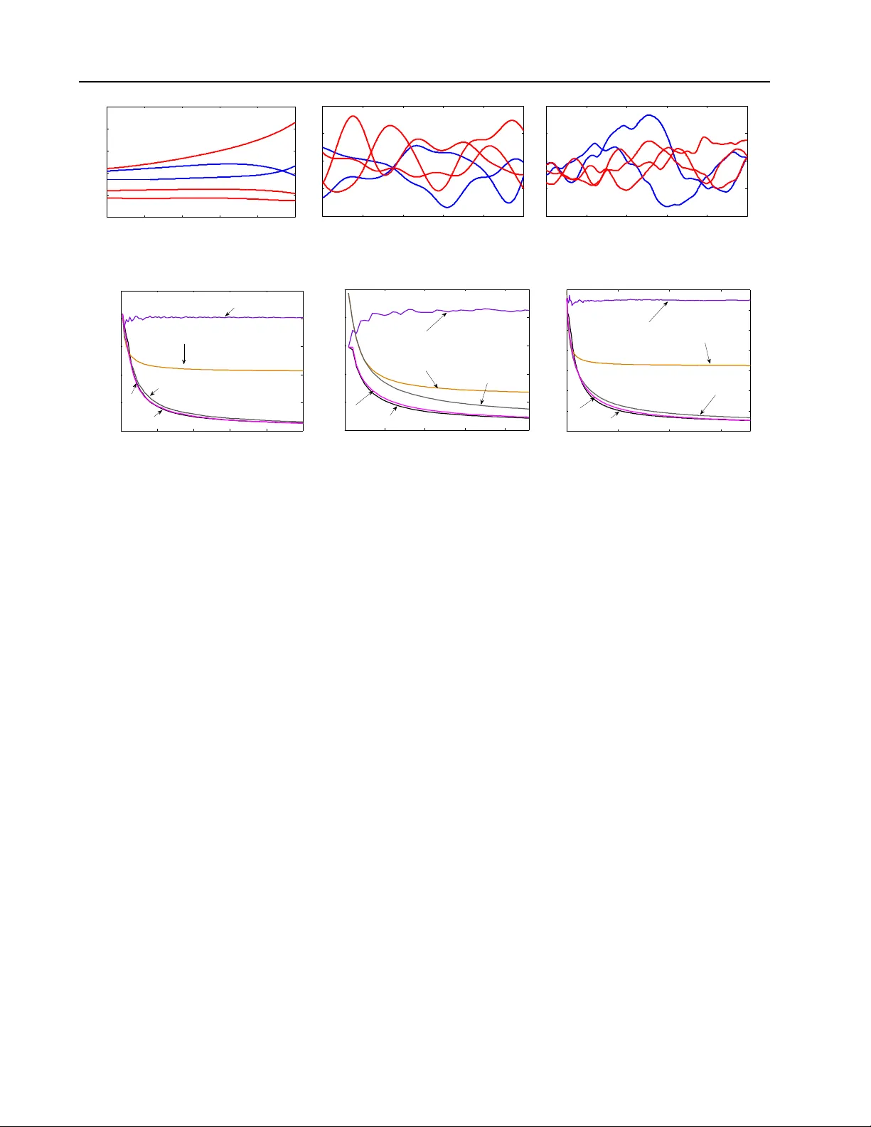
Gaussian Pro cess Optimization in the Bandit Setting: No Regret and Exp erimen tal Design Niranjan Sriniv as California Institute of T ec hnology niranjan@caltech.edu Andreas Krause California Institute of T ec hnology krausea@caltech.edu Sham M. Kak ade Univ ersity of P ennsylv ania skakade@wharton.upenn.edu Matthias Seeger Saarland Univ ersity mseeger@mmci.uni-saarland.de Abstract Man y applications require optimizing an un- kno wn, noisy function that is exp ensiv e to ev aluate. W e formalize this task as a multi- armed bandit problem, where the pa yoff function is either sampled from a Gaussian process (GP) or has lo w RKHS norm. W e resolve the imp or- tan t op en problem of deriving regret b ounds for this setting, which imply nov el conv ergence rates for GP optimization. W e analyze GP-UCB , an in tuitive upp er-confidence based algorithm, and b ound its cumulativ e regret in terms of maximal information gain, establishing a nov el connection b et w een GP optimization and exp erimen tal de- sign. Moreo ver, by b ounding the latter in terms of op erator sp ectra, we obtain explicit sublinear regret bounds for man y commonly used cov ari- ance functions. In some imp ortan t cases, our b ounds ha v e surprisingly weak dependence on the dimensionality . In our experiments on real sensor data, GP-UCB compares fav orably with other heuristical GP optimization approaches. 1. Introduction In most sto c hastic optimization settings, ev aluating the unkno wn function is exp ensiv e, and sampling is to be minimized. Examples include c ho osing adv ertisements in sponsored searc h to maximize profit in a click-through mo del ( Pandey & Olston , 2007 ) or learning optimal control strategies for rob ots ( Lizotte et al. , 2007 ). Predominan t approaches to this problem include the m ulti-armed bandit paradigm ( Robbins , 1952 ), where the goal is to maximize cumulativ e reward by optimally balancing exploration and exploitation, and exp erimen tal design ( Chaloner & V erdinelli , 1995 ), where the function is to b e explored globally with as few ev aluations as p ossible, for example by maximizing information 1 This is the longer version of our pap er in ICML 2010; see Sriniv as et al. ( 2010 ) gain. The challenge in b oth approaches is tw ofold: w e ha ve to estimate an unkno wn function f from noisy samples, and w e m ust optimize our estimate ov er some high-dimensional input space. F or the former, m uch progress has b een made in machine learning through k ernel metho ds and Gaussian pro cess (GP) models ( Rasm ussen & Williams , 2006 ), where smo othness assumptions about f are enco ded through the c hoice of kernel in a flexible nonparametric fashion. Beyond Euclidean spaces, kernels can b e defined on diverse domains such as spaces of graphs, sets, or lists. W e are concerned with GP optimization in the multi- armed bandit setting, where f is sampled from a GP distribution or has low “complexity” measured in terms of its RKHS norm under some kernel. W e pro- vide the first sublinear regret b ounds in this nonpara- metric setting, which imply con vergence rates for GP optimization. In particular, w e analyze the Gaussian Pro cess Upp er Confidence Bound ( GP-UCB ) algo- rithm, a simple and intuitiv e Bay esian metho d ( Auer et al. , 2002 ; Auer , 2002 ; Dani et al. , 2008 ). While ob jectives are different in the multi-armed bandit and exp erimen tal design paradigm, our results draw a close technical connection b et ween them: our regret b ounds come in terms of an information gain quantit y , measuring ho w fast f can b e learned in an information theoretic sense. The submodularity of this function allo ws us to pro ve sharp regret bounds for particular co v ariance functions, which w e demonstrate for com- monly used Squared Exp onen tial and Mat´ ern k ernels. Related W ork. Our work generalizes sto chastic line ar optimization in a bandit s etting, where the unkno wn function comes from a finite-dimensional linear space. GPs are nonlinear random functions, whic h can b e represented in an infinite-dimensional linear space. F or the standard linear setting, Dani et al. ( 2008 ) provide a near-c omplete characterization 1 (also see Auer 2002 ; Dani et al. 2007 ; Ab ernethy et al. 2008 ; Rusmevic hienton g & Tsitsiklis 2008 ), explicitly dep enden t on the dimensionality . In the GP setting, the challenge is to c haracterize complexity in a differ- en t manner, through prop erties of the kernel function. Our technical contributions are t wofold: first, we sho w how to analyze the nonlinear setting by fo cusing on the concept of information gain, and second, we explicitly b ound this information gain measure using the concept of submo dularit y ( Nemhauser et al. , 1978 ) and knowledge ab out kernel op erator sp ectra. Klein b erg et al. ( 2008 ) pro vide regret b ounds un- der w eaker and less configurable assumptions (only Lipsc hitz-contin uity w.r.t. a metric is assumed; Bub ec k et al. 2008 consider arbitrary top ological spaces), whic h ho wev er degrade rapidly with the di- mensionalit y of the problem (Ω( T d +1 d +2 )). In practice, linearit y w.r.t. a fixed basis is often to o stringent an assumption, while Lipsc hitz-contin uit y can b e to o coarse-grained, leading to p oor rate bounds. Adopting GP assumptions, w e can model levels of smoothness in a fine-grained w ay . F or example, our rates for the fre- quen tly used Squared Exponential kernel, enforcing a high degree of smoothness, ha ve weak dep endence on the dimensionality: O ( p T (log T ) d +1 ) (see Fig. 1 ). There is a large literature on GP (response surface) optimization. Several heuristics for trading off explo- ration and exploitation in GP optimization hav e b een prop osed (such as Exp ected Improv ement, Mo c kus et al. 1978 , and Most Probable Improv ement, Mo c kus 1989 ) and successfully applied in practice ( c.f. , Lizotte et al. 2007 ). Broch u et al. ( 2009 ) p rovide a comprehen- siv e review of and motiv ation for Bay esian optimiza- tion using GPs. The Efficien t Global Optimization (EGO) algorithm for optimizing exp ensiv e black-box functions is proposed by Jones et al. ( 1998 ) and ex- tended to GPs by Huang et al. ( 2006 ). Little is known ab out theoretical p erformance of GP optimization. While conv ergence of EGO is established b y V azquez & Bect ( 2007 ), conv ergence rates hav e remained elu- siv e. Gr ¨ unew¨ alder et al. ( 2010 ) consider the pure ex- ploration problem for GPs, where the goal is to find the optimal decision ov er T rounds, rather than maximize cum ulative rew ard (with no exploration/exploitation dilemma). They pro vide sharp b ounds for this explo- ration problem. Note that this metho dology w ould not lead to b ounds for minimizing the cumulativ e regret. Our cumulativ e regret b ounds translate to the first p erformance guarantees (rates) for GP optimization. Summary . Our main contributions are: • W e analyze GP-UCB , an intuitiv e algorithm for GP optimization, when the function is either sam- K ernel Linear k ernel RBF Matérn k ernel Regret R T � T (log T ) d +1 T ν + d ( d +1) 2 ν + d ( d +1) d √ T Figure 1. Our regret b ounds (up to polylog factors) for lin- ear, radial basis, and Mat´ ern k ernels — d is the dimension, T is the time horizon, and ν is a Mat´ ern parameter. pled from a known GP , or has lo w RKHS norm. • W e b ound the cumulativ e regret for GP-UCB in terms of the information gain due to sampling, establishing a no vel connection betw een exp eri- men tal design and GP optimization. • By b ounding the information gain for p opular classes of kernels, we establish sublinear regret b ounds for GP optimization for the first time. Our b ounds dep end on kernel choice and param- eters in a fine-grained fashion. • W e ev aluate GP-UCB on sensor netw ork data, demonstrating that it compares fa vorably to ex- isting algorithms for GP optimization. 2. Problem Statemen t and Background Consider the problem of sequen tially optimizing an un- kno wn rew ard function f : D → R : in eac h round t , we c ho ose a p oin t x t ∈ D and get to see the function v alue there, p erturb ed b y noise: y t = f ( x t ) +  t . Our goal is to maximize the sum of rewards P T t =1 f ( x t ), thus to p erform essentially as well as x ∗ = argmax x ∈ D f ( x ) (as rapidly as p ossible). F or example, w e might w ant to find lo cations of highest temp erature in a building b y sequentially activ ating sensors in a spatial netw ork and regressing on their measuremen ts. D consists of all sensor lo cations, f ( x ) is the temp erature at x , and sensor accuracy is quantified by the noise v ariance. Eac h activ ation draws battery p o wer, so we w an t to sample from as few sensors as p ossible. Regret. A natural p erformance metric in this con- text is cumulativ e regret, the loss in reward due to not kno wing f ’s maxim um p oints beforehand. Supp ose the unkno wn function is f , its maxim um p oin t 1 x ∗ = argmax x ∈ D f ( x ). F or our choice x t in round t , w e incur instantaneous regret r t = f ( x ∗ ) − f ( x t ). The cumulative r e gr et R T after T rounds is the sum of instan taneous regrets: R T = P T t =1 r t . A desirable asymptotic property of an algorithm is to be no-r e gr et : lim T →∞ R T /T = 0 . Note that neither r t nor R T are ev er revealed to the algorithm. Bounds on the av erage regret R T /T translate to con vergence rates for GP optimization: the maximum max t ≤ T f ( x t ) in the first T rounds is no further from f ( x ∗ ) than the av erage. 1 x ∗ need not b e unique; only f ( x ∗ ) o ccurs in the regret. 2.1. Gaussian Processes and RKHS’s Gaussian Pro cesses. Some assumptions on f are required to guarantee no-regret. While rigid paramet- ric assumptions such as linearit y ma y not hold in prac- tice, a certain degree of smo othness is often w arranted. In our sensor netw ork, temperature readings at closeb y lo cations are highly correlated (see Figure 2(a) ). W e can enforce implicit properties lik e smo othness with- out relying on any parametric assumptions, modeling f as a sample from a Gaussian pr o c ess (GP): a col- lection of dep enden t random v ariables, one for each x ∈ D , ev ery finite subset of which is m ultiv ariate Gaussian distributed in an ov erall consistent w ay ( Ras- m ussen & Williams , 2006 ). A GP ( µ ( x ) , k ( x , x 0 )) is sp ecified b y its mean function µ ( x ) = E [ f ( x )] and co v ariance (or k ernel) function k ( x , x 0 ) = E [( f ( x ) − µ ( x ))( f ( x 0 ) − µ ( x 0 ))]. F or GPs not conditioned on data, w e assume 2 that µ ≡ 0. Moreov er, we restrict k ( x , x ) ≤ 1, x ∈ D , i.e., w e assume b ounded v ariance. By fixing the correlation b eha vior, the co v ariance func- tion k enco des smo othness prop erties of sample func- tions f drawn from the GP . A range of commonly used k ernel functions is given in Section 5.2 . In this work, GPs play multiple roles. First, some of our results hold when the unkno wn target function is a sample from a known GP distribution GP(0 , k ( x , x 0 )). Second, the Bay esian algorithm we analyze generally uses GP(0 , k ( x , x 0 )) as prior distribution o ver f . A ma jor adv an tage of working with GPs is the exis- tence of simple analytic form ulae for mean and co- v ariance of the p osterior distribution, which allo ws easy implemen tation of algorithms. F or a noisy sam- ple y T = [ y 1 . . . y T ] T at points A T = { x 1 , . . . , x T } , y t = f ( x t ) +  t with  t ∼ N (0 , σ 2 ) i.i.d. Gaussian noise, the posterior ov er f is a GP distribution again, with mean µ T ( x ), cov ariance k T ( x , x 0 ) and v ariance σ 2 T ( x ): µ T ( x ) = k T ( x ) T ( K T + σ 2 I ) − 1 y T , (1) k T ( x , x 0 ) = k ( x , x 0 ) − k T ( x ) T ( K T + σ 2 I ) − 1 k T ( x 0 ) , σ 2 T ( x ) = k T ( x , x ) , (2) where k T ( x ) = [ k ( x 1 , x ) . . . k ( x T , x )] T and K T is the p ositiv e definite kernel matrix [ k ( x , x 0 )] x , x 0 ∈ A T . RKHS. Instead of the Ba yes case, where f is sam- pled from a GP prior, we also consider the more ag- nostic case where f has low “complexity” as measured under an RKHS norm (and distribution free assump- tions on the noise pro cess). The notion of r epr o duc- ing kernel Hilb ert sp ac es (RKHS, W ah ba 1990 ) is in- timately related to GPs and their cov ariance func- tions k ( x , x 0 ). The RKHS H k ( D ) is a complete sub- space of L 2 ( D ) of nicely b eha v ed functions, with an 2 This is w.l.o.g. ( Rasm ussen & Williams , 2006 ). inner product h· , ·i k ob eying the reproducing prop ert y: h f , k ( x , · ) i k = f ( x ) for all f ∈ H k ( D ). It is literally constructed by completing the set of mean functions µ T for all possible T , { x t } , and y T . The induced RKHS norm k f k k = p h f , f i k measures smoothness of f w.r.t. k : in muc h the same wa y as k 1 w ould generate smo other samples than k 2 as GP cov ariance functions, k · k k 1 assigns larger penalties than k · k k 2 . h· , ·i k can be extended to all of L 2 ( D ), in which case k f k k < ∞ iff f ∈ H k ( D ). F or most kernels discussed in Section 5.2 , mem b ers of H k ( D ) can uniformly appro ximate any con tinuous function on any compact subset of D . 2.2. Information Gain & Exp erimen tal Design One approach to maximizing f is to first choose p oin ts x t so as to estimate the function globally w ell, then pla y the maximum p oin t of our estimate. Ho w can we learn ab out f as rapidly as p ossible? This question comes do wn to Bay esian Exp erimen tal Design (henceforth “ED”; see Chaloner & V erdinelli 1995 ), where the informativ eness of a set of sampling p oin ts A ⊂ D ab out f is measured by the information gain (c.f., Cov er & Thomas 1991 ), whic h is the m utual information betw een f and observ ations y A = f A +  A at these p oints: I( y A ; f ) = H( y A ) − H( y A | f ) , (3) quan tifying the reduction in uncertaint y ab out f from rev ealing y A . Here, f A = [ f ( x )] x ∈ A and ε A ∼ N ( 0 , σ 2 I ). F or a Gaussian, H( N ( µ , Σ )) = 1 2 log | 2 π e Σ | , so that in our setting I( y A ; f ) = I( y A ; f A ) = 1 2 log | I + σ − 2 K A | , where K A = [ k ( x , x 0 )] x , x 0 ∈ A . While finding the information gain maximizer among A ⊂ D , | A | ≤ T is NP-hard ( Ko et al. , 1995 ), it can b e appro ximated by an efficien t greedy algorithm. If F ( A ) = I( y A ; f ), this algorithm pic ks x t = argmax x ∈ D F ( A t − 1 ∪{ x } ) in round t , whic h can b e shown to b e equiv alent to x t = argmax x ∈ D σ t − 1 ( x ) , (4) where A t − 1 = { x 1 , . . . , x t − 1 } . Importantly , this simple algorithm is guaran teed to find a near-optimal solution: for the set A T obtained after T rounds, we ha ve that F ( A T ) ≥ (1 − 1 /e ) max | A |≤ T F ( A ) , (5) at least a constant fraction of the optimal infor- mation gain v alue. This is b ecause F ( A ) satisfies a diminishing returns prop ert y called submo dularity ( Krause & Guestrin , 2005 ), and the greedy approxima- tion guaran tee ( 5 ) holds for any submo dular function ( Nemhauser et al. , 1978 ). While sequen tially optimizing Eq. 4 is a prov ably goo d w ay to explor e f globally , it is not well suited for func- tion optimization. F or the latter, we only need to iden- tify p oints x where f ( x ) is large, in order to concen- trate sampling there as rapidly as p ossible, th us exploit our knowledge about maxima. In fact, the ED rule ( 4 ) do es not ev en dep end on observ ations y t obtained along the w ay . Nev ertheless, the maximum informa- tion gain after T rounds will pla y a prominen t role in our regret b ounds, forging an imp ortan t connection b et w een GP optimization and exp erimen tal design. 3. GP-UCB Algorithm F or sequential optimization, the ED rule ( 4 ) can b e w asteful: it aims at decreasing uncertain t y globally , not just where maxima migh t be. Another idea is to pic k points as x t = argmax x ∈ D µ t − 1 ( x ), maximizing the exp ected reward based on the p osterior so far. Ho wev er, this rule is to o greedy to o so on and tends to get stuck in shallow lo cal optima. A combined strategy is to choose x t = argmax x ∈ D µ t − 1 ( x ) + β 1 / 2 t σ t − 1 ( x ) , (6) where β t are appropriate constants. This latter ob jec- tiv e prefers b oth p oints x where f is uncertain (large σ t − 1 ( · )) and such where we exp ect to ac hieve high rew ards (large µ t − 1 ( · )): it implicitly negotiates the exploration–exploitation tradeoff. A natural interpre- tation of this sampling rule is that it greedily selects p oin ts x such that f ( x ) should b e a reasonable upp er b ound on f ( x ∗ ), since the argument in ( 6 ) is an upp er quan tile of the marginal p osterior P ( f ( x ) | y t − 1 ). W e call this choice the Gaussian pr o c ess upp er c onfidenc e b ound rule ( GP-UCB ), where β t is sp ecified dep ending on the context (see Section 4 ). Pseudo code for the GP-UCB algorithm is pro vided in Algorithm 1 . Figure 2 illustrates tw o subsequen t iterations, where GP-UCB b oth explores (Figure 2(b) ) by sampling an input x with large σ 2 t − 1 ( x ) and exploits (Figure 2(c) ) b y sampling x with large µ t − 1 ( x ). The GP-UCB selection rule Eq. 6 is motiv ated by the UCB algorithm for the classical m ulti-armed bandit problem ( Auer et al. , 2002 ; Ko csis & Szep esv´ ari , 2006 ). Among comp eting criteria for GP optimization (see Section 1 ), a v ariant of the GP-UCB rule has b een demonstrated to b e effectiv e for this application ( Dorard et al. , 2009 ). T o our knowledge, strong theoretical results of the kind provided for GP-UCB in this pap er hav e not b een given for any of these search heuristics. In Section 6 , we sho w that in practice GP-UCB compares fav orably with these alternatives. If D is infinite, finding x t in ( 6 ) ma y be hard: the upp er confidence index is m ultimo dal in general. Ho wev er, global searc h heuristics are v ery effective in practice ( Bro ch u et al. , 2009 ). It is generally assumed Algorithm 1 The GP-UCB algorithm. Input: Input space D ; GP Prior µ 0 = 0 , σ 0 , k for t = 1 , 2 , . . . do Cho ose x t = argmax x ∈ D µ t − 1 ( x ) + p β t σ t − 1 ( x ) Sample y t = f ( x t ) +  t P erform Ba yesian up date to obtain µ t and σ t end for that ev aluating f is more costly than maximizing the UCB index. UCB algorithms (and GP optimization tec hniques in general) hav e b een applied to a large num b er of problems in practice ( Ko csis & Szep esv´ ari , 2006 ; P andey & Olston , 2007 ; Lizotte et al. , 2007 ). Their p erformance is well characterized in b oth the finite arm setting and the linear optimization setting, but no conv ergence rates for GP optimization are known. 4. Regret Bounds W e now establish cumulativ e regret b ounds for GP optimization, treating a n umber of differen t settings: f ∼ GP(0 , k ( x , x 0 )) for finite D , f ∼ GP(0 , k ( x , x 0 )) for general compact D , and the agnostic case of arbi- trary f with b ounded RKHS norm. GP optimization generalizes sto chastic linear opti- mization, where a function f from a finite-dimensional linear space is optimized ov er. F or the linear case, Dani et al. ( 2008 ) provide regret b ounds that explicitly de- p end on the dimensionality 3 d . GPs can b e seen as random functions in some infinite-dimensional linear space, so their results do not apply in this case. This problem is circum ven ted in our regret b ounds. The quan tity gov erning them is the maximum information gain γ T after T rounds, defined as: γ T := max A ⊂ D : | A | = T I( y A ; f A ) , (7) where I( y A ; f A ) = I( y A ; f ) is defined in ( 3 ). Recall that I( y A ; f A ) = 1 2 log | I + σ − 2 K A | , where K A = [ k ( x , x 0 )] x , x 0 ∈ A is the cov ariance matrix of f A = [ f ( x )] x ∈ A asso ciated with the samples A . Our regret b ounds are of the form O ∗ ( √ T β T γ T ), where β T is the confidence parameter in Algorithm 1 , while the b ounds of Dani et al. ( 2008 ) are of the form O ∗ ( √ T β T d ) ( d the dimensionality of the linear function space). Here and b elo w, the O ∗ notation is a v ariant of O , where log factors are suppressed. While our pro ofs – all pro- vided in the App endix – use techniques similar to those of Dani et al. ( 2008 ), w e face a num b er of additional 3 In general, d is the dimensionality of the input space D , which in the finite-dimensional linear case coincides with the feature space. 0 10 20 30 40 0 10 20 30 40 15 20 25 Temperature (C) (a) T emp er atur e data − 6 − 4 − 2 0 2 4 6 − 5 − 4 − 3 − 2 − 1 0 1 2 3 4 5 (b) Iter ation t − 6 − 4 − 2 0 2 4 6 − 5 − 4 − 3 − 2 − 1 0 1 2 3 4 5 (c) Iter ation t + 1 Figure 2. (a) Example of temp erature data collected b y a net work of 46 sensors at In tel Researc h Berkeley . (b,c) Two iterations of the GP-UCB algorithm. It samples p oin ts that are either uncertain (b) or hav e high p osterior mean (c). significan t tec hnical c hallenges. Besides a voiding the finite-dimensional analysis, we must handle confidence issues, which are more delicate for nonlinear random functions. Imp ortan tly , note that the information gain is a prob- lem dep enden t quantit y — prop erties of b oth the ker- nel and the input space will determine the gro wth of regret. In Section 5 , w e provide general metho ds for b ounding γ T , either b y efficien t auxiliary computa- tions or by direct expressions for specific kernels of in terest. Our results matc h known low er b ounds (up to log factors) in b oth the K -armed bandit and the d -dimensional linear optimization case. Bounds for a GP Prior. F or finite D , we obtain the following b ound. Theorem 1 L et δ ∈ (0 , 1) and β t = 2 log( | D | t 2 π 2 / 6 δ ) . Ru nning GP-UCB with β t for a sample f of a GP with me an function zer o and c ovarianc e function k ( x , x 0 ) , we obtain a r e gr et b ound of O ∗ ( p T γ T log | D | ) with high pr ob ability. Pr e cisely, Pr n R T ≤ p C 1 T β T γ T ∀ T ≥ 1 o ≥ 1 − δ. wher e C 1 = 8 / log(1 + σ − 2 ) . The pro of methodology follo ws Dani et al. ( 2007 ) in that we relate the regret to the gro wth of the log v olume of the confidence ellipsoid — a no velt y in our pro of is sho wing how this gro wth is c haracterized by the information gain. This theorem sho ws that, with high probabilit y ov er samples from the GP , the cumulativ e regret is b ounded in terms of the maxim um information gain, forging a no vel connection b et ween GP optimization and exp er- imen tal design. This link is of fundamental technical imp ortance, allo wing us to generalize Theorem 1 to infinite decision spaces. Moreo ver, the submo dularity of I( y A ; f A ) allows us to derive sharp a priori b ounds, dep ending on c hoice and parameterization of k (see Section 5 ). In the follo wing theorem, we generalize our result to any compact and conv ex D ⊂ R d under mild assumptions on the kernel function k . Theorem 2 L et D ⊂ [0 , r ] d b e c omp act and c onvex, d ∈ N , r > 0 . Supp ose that the kernel k ( x , x 0 ) satisfies the fol lowing high pr ob ability b ound on the derivatives of GP sample p aths f : for some c onstants a, b > 0 , Pr { sup x ∈ D | ∂ f /∂ x j | > L } ≤ ae − ( L/b ) 2 , j = 1 , . . . , d. Pick δ ∈ (0 , 1) , and define β t = 2 log( t 2 2 π 2 / (3 δ )) + 2 d log  t 2 dbr p log(4 da/δ )  . Ru nning the GP-UCB with β t for a sample f of a GP with me an function zer o and c ovarianc e function k ( x , x 0 ) , we obtain a r e gr et b ound of O ∗ ( √ dT γ T ) with high pr ob ability. Pr e cisely, with C 1 = 8 / log(1 + σ − 2 ) we have Pr n R T ≤ p C 1 T β T γ T + 2 ∀ T ≥ 1 o ≥ 1 − δ. The main c hallenge in our pro of (provided in the Ap- p endix) is to lift the regret bound in terms of the confidence ellipsoid to general D . The smoothness assumption on k ( x , x 0 ) disqualifies GPs with highly erratic sample paths. It holds for stationary kernels k ( x , x 0 ) = k ( x − x 0 ) whic h are four times differen- tiable (Theorem 5 of Ghosal & Roy ( 2006 )), such as the Squared Exp onen tial and Mat ´ ern k ernels with ν > 2 (see Section 5.2 ), while it is violated for the Ornstein- Uhlen b ec k kernel (Mat ´ ern with ν = 1 / 2; a stationary v ariant of the Wiener pro cess). F or the latter, sam- ple paths f are nondifferen tiable almost ev erywhere with probabilit y one and come with indep enden t in- cremen ts. W e conjecture that a result of the form of Theorem 2 do es not hold in this case. Bounds for Arbitrary f in the RKHS. Thus far, w e hav e assumed that the target function f is sampled from a GP prior and that the noise is N (0 , σ 2 ) with kno wn v ariance σ 2 . W e now analyze GP-UCB in an agnostic setting, where f is an arbitrary function from the RKHS corresp onding to kernel k ( x , x 0 ). Moreo ver, we allow the noise v ariables ε t to b e an ar- bitrary martingale difference sequence (meaning that E [ ε t | ε 1 : γ T = O  T d ( d +1) / (2 ν + d ( d +1)) (log T )  . A pro of of Theorem 5 is given in the App endix, , we only sketc h the idea here. γ T is b ounded by Theo- rem 4 in terms the eigendeca y of the kernel matrix K D . If D is infinite or v ery large, we can use the op erator sp ectrum of k ( x , x 0 ), which likewise deca ys rapidly . F or the kernels of interest here, asymptotic expressions for the op erator eigenv alues are given in Seeger et al. ( 2008 ), who deriv ed b ounds on the information gain for fixed and random designs (in con trast to the worst-case information gain considered here, which is substantially more challenging to b ound). The main challenge in the pro of is to ensure the existence of discretizations D T ⊂ D , dense in the limit, for which tail sums B ( T ∗ ) /n T in Theorem 4 are close to corresp onding op erator sp ectra tail sums. T ogether with Theorems 2 and 3 , this result guaran- tees sublinear regret of GP-UCB for any dimension (see Figure 1 ). F or the Squared Exponential kernel, the dimension d app ears as exp onen t of log T only , so that the regret gro ws at most as O ∗ ( √ T (log T ) d +1 2 ) – the high degree of smo othness of the sample paths effectiv ely com bats the curse of dimensionality . 6. Exp erimen ts W e compare GP-UCB with heuristics such as the Exp ected Improv ement (EI) and Most Probable Impro vemen t (MPI), and with naiv e metho ds which c ho ose p oin ts of maximum mean or v ariance only , b oth on syn thetic and real sensor netw ork data. F or synthetic data, we sample random functions from a squared exponential kernel with lengthscale parameter 0 . 2. The sampling noise v ariance σ 2 w as set to 0 . 025 or 5% of the signal v ariance. Our decision set D = [0 , 1] is uniformly discretized into 1000 p oin ts. W e run eac h algorithm for T = 1000 iterations with δ = 0 . 1, a veraging ov er 30 trials (samples from the k ernel). While the choice of β t as recommended by Theorem 1 leads to comp etitiv e performance of GP-UCB , we find (using cross-v alidation) that the algorithm is impro ved by scaling β t do wn b y a factor 5. Note that w e did not optimize constants in our regret b ounds. Next, we use temp erature data collected from 46 sen- sors deplo y ed at In tel Research Berkeley o ver 5 da ys at 1 min ute in terv als, p ertaining to the example in Sec- tion 2 . W e tak e the first tw o-thirds of the data set to compute the empirical cov ariance of the sensor read- ings, and use it as the kernel matrix. The functions f for optimization consist of one set of observ ations from all the sensors taken from the remaining third of the 0 0.2 0.4 0.6 0.8 1 −4 −2 0 2 4 6 (a) Bayesian Line ar R e gr ession 0 0.2 0.4 0.6 0.8 1 −2 −1 0 1 2 (b) Squar e d Exp onential 0 0.2 0.4 0.6 0.8 1 −2 −1 0 1 2 (c) Mat´ ern Figure 4. Sample functions drawn from a GP with linear, squared exp onen tial and Mat´ ern kernels ( ν = 2 . 5.) 0 20 40 60 80 100 0 0.2 0.4 0.6 0.8 1 Iterations Mean Average Regret Var only Mean only MPI EI UCB (a) Squar e d exp onential 0 10 20 30 40 0 1 2 3 4 5 Iterations Mean Average Regret Var only Mean only MPI EI UCB (b) T emp er atur e data 0 100 200 300 0 5 10 15 20 25 30 35 Iterations Mean Average Regret EI MPI Var only Mean only UCB (c) T r affic data Figure 5. Comparison of p erformance: GP-UCB and v arious heuristics on synthetic (a), and sensor netw ork data (b, c). data set, and the results (for T = 46 , σ 2 = 0 . 5 or 5% noise, δ = 0 . 1) w ere a veraged ov er 2000 p ossible c hoices of the ob jectiv e function. Lastly , w e take data from traffic sensors deploy ed along the highw a y I-880 South in California. The goal w as to find the point of minimum speed in order to iden tify the most congested p ortion of the highw ay; we used traffic speed data for all w orking da ys from 6 AM to 11 AM for one month, from 357 sensors. W e again use the cov ariance matrix from tw o-thirds of the data set as kernel matrix, and test on the other third. The results (for T = 357 , σ 2 = 4 . 78 or 5% noise, δ = 0 . 1) w ere a veraged ov er 900 runs. Figure 5 compares the mean av erage regret incurred b y the different heuristics and the GP-UCB algorithm on synthetic and real data. F or temperature data, the GP-UCB algorithm and EI heuristic clearly outp erform the others, and do not exhibit significant difference b etw een each other. On synthetic and traf- fic data MPI do es equally well. In summary , GP-UCB p erforms at least on par with the existing approaches whic h are not equipp ed with regret b ounds. 7. Conclusions W e pro ve the first sublinear regret b ounds for GP optimization with commonly used k ernels (see Fig- ure 1 ), b oth for f sampled from a known GP and f of lo w RKHS norm. W e analyze GP-UCB , an in tuitive, Ba yesian upp er confidence b ound based sampling rule. Our regret b ounds crucially depend on the information gain due to sampling, establishing a no vel connection b et w een bandit optimization and exp erimen tal design. W e b ound the information gain in terms of the kernel sp ectrum, providing a general metho dology for obtain- ing regret b ounds with kernels of interest. Our exp er- imen ts on real sensor net work data indicate that GP- UCB p erforms at least on par with comp eting criteria for GP optimization, for which no regret b ounds are kno wn at presen t. Our results provide an interesting step tow ards understanding exploration–exploitation tradeoffs with complex utility functions. Ac kno wledgements W e thank Marcus Hutter for insigh tful comments on an earlier version of this paper. This researc h was partially supp orted by ONR grant N00014-09-1-1044, NSF gran t CNS-0932392, a gift from Microsoft Cor- p oration and the Excellence Initiative of the German researc h foundation (DFG). References Ab erneth y , J., Hazan, E., and Rakhlin, A. An efficient algorithm for linear bandit optimization, 2008. COL T. Auer, P . Using confidence bounds for exploitation- exploration trade-offs. JMLR , 3:397–422, 2002. Auer, P ., Cesa-Bianc hi, N., and Fischer, P . Finite-time analysis of the multiarmed bandit problem. Mach. L earn. , 47(2-3):235–256, 2002. Bro c h u, E., Cora, M., and de F reitas, N. A tutorial on Ba yesian optimization of exp ensive cost functions, with application to active user mo deling and hierarchical re- inforcemen t learning. In TR-2009-23, UBC , 2009. Bub ec k, S., Munos, R., Stoltz, G., and Szep esv´ ari, C. On- line optimization in X-armed bandits. In NIPS , 2008. Chaloner, K. and V erdinelli, I. Ba yesian exp erimen tal de- sign: A review. Stat. Sci. , 10(3):273–304, 1995. Co ver, T. M. and Thomas, J. A. Elements of Information The ory . Wiley Interscience, 1991. Dani, V., Hay es, T. P ., and Kak ade, S. The price of bandit information for online optimization. In NIPS , 2007. Dani, V., Ha yes, T. P ., and Kak ade, S. M. Sto c hastic linear optimization under bandit feedback. In COL T , 2008. Dorard, L., Glow ack a, D., and Shaw e-T aylor, J. Gaussian pro cess mo delling of dependencies in multi-armed bandit problems. In Int. Symp. Op. R es. , 2009. F reedman, D. A. On tail probabilities for martingales. Ann. Pr ob. , 3(1):100–118, 1975. Ghosal, S. and Roy , A. Posterior consistency of Gaussian pro cess prior for nonparametric binary regression. Ann. Stat. , 34(5):2413–2429, 2006. Gr ¨ unew¨ alder, S., Audib ert, J-Y., Opp er, M., and Shaw e- T aylor, J. Regret bounds for gaussian pro cess bandit problems. In AIST A TS , 2010. Huang, D., Allen, T. T., Notz, W. I., and Zeng, N. Global optimization of sto chastic black-box systems via sequen- tial kriging meta-mo dels. J Glob. Opt. , 34:441–466, 2006. Jones, D. R., Sc honlau, M., and W elch, W. J. Efficient global optimization of exp ensiv e black-box functions. J Glob. Opti. , 13:455–492, 1998. Klein b erg, R., Slivkins, A., and Upfal, E. Multi-armed bandits in metric spaces. In STOC , pp. 681–690, 2008. Ko, C., Lee, J., and Queyranne, M. An exact algorithm for maxim um entrop y sampling. Ops R es , 43(4):684–691, 1995. Ko csis, L. and Szep esv´ ari, C. Bandit based monte-carlo planning. In ECML , 2006. Krause, A. and Guestrin, C. Near-optimal nonmy opic v alue of information in graphical mo dels. In UAI , 2005. Lizotte, D., W ang, T., Bowling, M., and Sc huurmans, D. Automatic gait optimization with Gaussian pro cess re- gression. In IJCAI , pp. 944–949, 2007. McDiarmid, C. Conc entration. In Pr ob abilistiic Metho ds for Algorithmic Discr ete Mathematics . Springer, 1998. Mo c kus, J. Bayesian Appr o ach to Glob al Optimization . Klu wer Academic Publishers, 1989. Mo c kus, J., Tiesis, V., and Zilinsk as, A. T owar d Glob al Optimization , v olume 2, chapter Bay esian Methods for Seeking the Extremum, pp. 117–128. 1978. Nemhauser, G., W olsey , L., and Fisher, M. An analysis of the appro ximations for maximizing submodular set functions. Math. Pr o g. , 14:265–294, 1978. P andey , S. and Olston, C. Handling advertisemen ts of un- kno wn quality in search advertising. In NIPS . 2007. Rasm ussen, C. E. and Williams, C. K. I. Gaussian Pr o- c esses for Machine L e arning . MIT Press, 2006. Robbins, H. Some asp ects of the sequen tial design of ex- p erimen ts. Bul. Am. Math. So c. , 58:527–535, 1952. Rusmevic hientong, P . and Tsitsiklis, J. N. Linearly param- eterized bandits. abs/0812.3465, 2008. Seeger, M. W., Kak ade, S. M., and F oster, D. P . Infor- mation consistency of nonparametric Gaussian process metho ds. IEEE T r. Inf. The o. , 54(5):2376–2382, 2008. Sha we-T aylor, J., Williams, C., Cristianini, N., and Kan- dola, J. On the eigensp ectrum of the Gram matrix and the generalization error of k ernel-PCA. IEEE T r ans. Inf. The o. , 51(7):2510–2522, 2005. Sriniv as, N., Krause, A., Kak ade, S., and Seeger, M. Gaus- sian pro cess optimization in the bandit setting: No re- gret and exp erimental design. In ICML , 2010. Stein, M. Interp olation of Sp atial Data: Some Theory for Kriging . Springer, 1999. V azquez, E. and Bect, J. Con vergence prop erties of the exp ected improv ement algorithm, 2007. W ahba, G. Spline Mo dels for Observational Data . SIAM, 1990. A. Regret Bounds for T arget F unction Sampled from GP In this section, we provide details for the pro ofs of Theorem 1 and Theorem 2 . In b oth cases, the strategy is to show that | f ( x ) − µ t − 1 ( x ) | ≤ β 1 / 2 t σ t − 1 ( x ) for all t ∈ N and all x ∈ D , or in the infinite case, all x in a discretization of D whic h b ecomes dense as t gets large. A.1. Finite Decision Set W e b egin with the finite case, | D | < ∞ . Lemma 5.1 Pick δ ∈ (0 , 1) and set β t = 2 log( | D | π t /δ ) , wher e P t ≥ 1 π − 1 t = 1 , π t > 0 . Then, | f ( x ) − µ t − 1 ( x ) | ≤ β 1 / 2 t σ t − 1 ( x ) ∀ x ∈ D ∀ t ≥ 1 holds with pr ob ability ≥ 1 − δ . Pro of Fix t ≥ 1 and x ∈ D . Conditioned on y t − 1 = ( y 1 , . . . , y t − 1 ), { x 1 , . . . , x t − 1 } are deterministic, and f ( x ) ∼ N ( µ t − 1 ( x ) , σ 2 t − 1 ( x )). Now, if r ∼ N (0 , 1), then Pr { r > c } = e − c 2 / 2 (2 π ) − 1 / 2 Z e − ( r − c ) 2 / 2 − c ( r − c ) dr ≤ e − c 2 / 2 Pr { r > 0 } = (1 / 2) e − c 2 / 2 for c > 0, since e − c ( r − c ) ≤ 1 for r ≥ c . Therefore, Pr {| f ( x ) − µ t − 1 ( x ) | > β 1 / 2 t σ t − 1 ( x ) } ≤ e − β t / 2 , using r = ( f ( x ) − µ t − 1 ( x )) /σ t − 1 ( x ) and c = β 1 / 2 t . Applying the union b ound, | f ( x ) − µ t − 1 ( x ) | ≤ β 1 / 2 t σ t − 1 ( x ) ∀ x ∈ D holds with probability ≥ 1 − | D | e − β t / 2 . Cho osing | D | e − β t / 2 = δ/π t and using the union bound for t ∈ N , the statement holds. F or example, w e can use π t = π 2 t 2 / 6. Lemma 5.2 Fix t ≥ 1 . If | f ( x ) − µ t − 1 ( x ) | ≤ β 1 / 2 t σ t − 1 ( x ) for al l x ∈ D , then the r e gr et r t is b ounde d by 2 β 1 / 2 t σ t − 1 ( x t ) . Pro of By definition of x t : µ t − 1 ( x t ) + β 1 / 2 t σ t − 1 ( x t ) ≥ µ t − 1 ( x ∗ ) + β 1 / 2 t σ t − 1 ( x ∗ ) ≥ f ( x ∗ ). Therefore, r t = f ( x ∗ ) − f ( x t ) ≤ β 1 / 2 t σ t − 1 ( x t ) + µ t − 1 ( x t ) − f ( x t ) ≤ 2 β 1 / 2 t σ t − 1 ( x t ) . Lemma 5.3 The information gain for the p oints se- le cte d c an b e expr esse d in terms of the pr e dictive vari- anc es. If f T = ( f ( x t )) ∈ R T : I( y T ; f T ) = 1 2 X T t =1 log  1 + σ − 2 σ 2 t − 1 ( x t )  . Pro of Recall that I( y T ; f T ) = H( y T ) − (1 / 2) log | 2 πeσ 2 I | . No w, H( y T ) = H( y T − 1 ) + H( y T | y T − 1 ) = H( y T − 1 ) + log (2 πe ( σ 2 + σ 2 t − 1 ( x T ))) / 2. Here, w e use that x 1 , . . . , x T are deterministic con- ditioned on y T − 1 , and that the conditional v ariance σ 2 T − 1 ( x T ) do es not dep end on y T − 1 . The res ult fol- lo ws b y induction. Lemma 5.4 Pick δ ∈ (0 , 1) and let β t b e define d as in L emma 5.1 . Then, the fol lowing holds with pr ob ability ≥ 1 − δ : X T t =1 r 2 t ≤ β T C 1 I( y T ; f T ) ≤ C 1 β T γ T ∀ T ≥ 1 , wher e C 1 := 8 / log(1 + σ − 2 ) ≥ 8 σ 2 . Pro of By Lemma 5.1 and Lemma 5.2 , we hav e that { r 2 t ≤ 4 β t σ 2 t − 1 ( x t ) ∀ t ≥ 1 } with probability ≥ 1 − δ . No w, β t is nondecreasing, so that 4 β t σ 2 t − 1 ( x t ) ≤ 4 β T σ 2 ( σ − 2 σ 2 t − 1 ( x t )) ≤ 4 β T σ 2 C 2 log(1 + σ − 2 σ 2 t − 1 ( x t )) with C 2 = σ − 2 / log(1 + σ − 2 ) ≥ 1, since s 2 ≤ C 2 log(1 + s 2 ) for s ∈ [0 , σ − 2 ], and σ − 2 σ 2 t − 1 ( x t ) ≤ σ − 2 k ( x t , x t ) ≤ σ − 2 . Noting that C 1 = 8 σ 2 C 2 , the result follows by plugging in the represen tation of Lemma 5.3 . Finally , Theorem 1 is a simple consequence of Lemma 5.4 , since R 2 T ≤ T P T t =1 r 2 t b y the Cauch y- Sc hw arz inequality . A.2. General Decision Set Theorem 2 extends the statemen t of Theorem 1 to the general case of D ⊂ R d compact. W e cannot exp ect this generalization to work without an y as- sumptions on the k ernel k ( x , x 0 ). F or example, if k ( x , x 0 ) = e −k x − x 0 k (Ornstein-Uhlen b ec k), while sam- ple paths f are a.s. contin uous, they are still very er- ratic: f is a.s. nondifferen tiable almost everywhere, and the pro cess comes with independent incremen ts, a stationary v ariant of Bro wnian motion. The additional assumption on k in Theorem 2 is rather mild and is satisfied b y sev eral common kernels, as discussed in Section 4 . Recall that the finite case proof is based on Lemma 5.1 pa ving the wa y for Lemma 5.2 . How ever, Lemma 5.1 do es not hold for infinite D . First, let us observe that w e ha ve confidence on all decisions actually chosen. Lemma 5.5 Pick δ ∈ (0 , 1) and set β t = 2 log( π t /δ ) , wher e P t ≥ 1 π − 1 t = 1 , π t > 0 . Then, | f ( x t ) − µ t − 1 ( x t ) | ≤ β 1 / 2 t σ t − 1 ( x t ) ∀ t ≥ 1 holds with pr ob ability ≥ 1 − δ . Pro of Fix t ≥ 1 and x ∈ D . Conditioned on y t − 1 = ( y 1 , . . . , y t − 1 ), { x 1 , . . . , x t − 1 } are determin- istic, and f ( x ) ∼ N ( µ t − 1 ( x ) , σ 2 t − 1 ( x )). As b efore, Pr {| f ( x t ) − µ t − 1 ( x t ) | > β 1 / 2 t σ t − 1 ( x t ) } ≤ e − β t / 2 . Since e − β t / 2 = δ /π t and using the union b ound for t ∈ N , the statement holds. Purely for the sake of analysis, w e use a set of dis- cretizations D t ⊂ D , where D t will be used at time t in the analysis. Essentially , w e use this to obtain a v alid confidence in terv al on x ∗ . The following lemma pro vides a confidence b ound for these subsets. Lemma 5.6 Pick δ ∈ (0 , 1) and set β t = 2 log( | D t | π t /δ ) , wher e P t ≥ 1 π − 1 t = 1 , π t > 0 . Then, | f ( x ) − µ t − 1 ( x ) | ≤ β 1 / 2 t σ t − 1 ( x ) ∀ x ∈ D t , ∀ t ≥ 1 holds with pr ob ability ≥ 1 − δ . Pro of The pro of is iden tical to that in Lemma 5.1 , except now we use D t at each timestep. No w by assumption and the union bound, w e ha ve that Pr {∀ j, ∀ x ∈ D , | ∂ f / ( ∂ x j ) | < L } ≥ 1 − dae − L 2 /b 2 . whic h implies that, with probabilit y greater than 1 − dae − L 2 /b 2 , we hav e that ∀ x ∈ D , | f ( x ) − f ( x 0 ) | ≤ L k x − x 0 k 1 . (9) This allows us to obtain confidence on x ? as follows. No w let us c ho ose a discretization D t of size ( τ t ) d so that for all x ∈ D t k x − [ x ] t k 1 ≤ r d/τ t where [ x ] t denotes the closest p oin t in D t to x . A suf- ficien t discretization has eac h coordinate with τ t uni- formly spaced p oints. Lemma 5.7 Pick δ ∈ (0 , 1) and set β t = 2 log(2 π t /δ ) + 4 d log ( dtbr p log(2 da/δ )) , wher e P t ≥ 1 π − 1 t = 1 , π t > 0 . L et τ t = dt 2 br p log(2 da/δ ) L et [ x ∗ ] t denotes the closest p oint in D t to x ∗ . Henc e, Then, | f ( x ∗ ) − µ t − 1 ([ x ∗ ] t ) | ≤ β 1 / 2 t σ t − 1 ([ x ∗ ] t ) + 1 t 2 ∀ t ≥ 1 holds with pr ob ability ≥ 1 − δ . Pro of Using ( 9 ), w e hav e that with probability greater than 1 − δ / 2, ∀ x ∈ D , | f ( x ) − f ( x 0 ) | ≤ b p log(2 da/δ ) k x − x 0 k 1 . Hence, ∀ x ∈ D t , | f ( x ) − f ([ x ] t ) | ≤ r db p log(2 da/δ ) /τ t . No w b y c ho osing τ t = dt 2 br p log(2 da/δ ), we ha ve that ∀ x ∈ D t , | f ( x ) − f ([ x ] t ) | ≤ 1 t 2 This implies that | D t | = ( dt 2 br p log(2 da/δ )) d . Using δ / 2 in Lemma 5.6 , we can apply the confidence b ound to [ x ∗ ] t (as this lives in D t ) to obtain the result. No w w e are able to b ound the regret. Lemma 5.8 Pick δ ∈ (0 , 1) and set β t = 2 log(4 π t /δ ) + 4 d log ( dtbr p log(4 da/δ )) , wher e P t ≥ 1 π − 1 t = 1 , π t > 0 . Then, with pr ob ability gr e ater than 1 − δ , for al l t ∈ N , the r e gr et is b ounde d as fol lows: r t ≤ 2 β 1 / 2 t σ t − 1 ( x t ) + 1 t 2 . Pro of W e use δ / 2 in both Lemma 5.5 and Lemma 5.7 , so that these even ts hold with probability greater than 1 − δ . Note that the sp ecification of β t in the ab o v e lemma is greater than the sp ecification used in Lemma 5.5 (with δ / 2), so this c hoice is v alid. By definition of x t : µ t − 1 ( x t ) + β 1 / 2 t σ t − 1 ( x t ) ≥ µ t − 1 ([ x ∗ ] t ) + β 1 / 2 t σ t − 1 ([ x ∗ ] t ). Also, by Lemma 5.7 , we ha ve that µ t − 1 ([ x ∗ ] t ) + β 1 / 2 t σ t − 1 ([ x ∗ ] t ) + 1 /t 2 ≥ f ( x ∗ ), whic h implies µ t − 1 ( x t ) + β 1 / 2 t σ t − 1 ( x t ) ≥ f ( x ∗ ) − 1 /t 2 . Therefore, r t = f ( x ∗ ) − f ( x t ) ≤ β 1 / 2 t σ t − 1 ( x t ) + 1 /t 2 + µ t − 1 ( x t ) − f ( x t ) ≤ 2 β 1 / 2 t σ t − 1 ( x t ) + 1 /t 2 . whic h completes the pro of. No w we are ready to complete the proof of Theorem 2 . As shown in the pro of of Lemma 5.4 , w e hav e that with probabilit y greater than 1 − δ , X T t =1 4 β t σ 2 t − 1 ( x t ) ≤ C 1 β T γ T ∀ T ≥ 1 , so that by Cauc hy-Sc hw arz: X T t =1 2 β 1 / 2 t σ t − 1 ( x t ) ≤ p C 1 T β T γ T ∀ T ≥ 1 , Hence, X T t =1 r t ≤ p C 1 T β T γ T + π 2 / 6 ∀ T ≥ 1 , (since P 1 /t 2 = π 2 / 6). Theorem 2 no w follo ws. Finally , w e now discuss the additional assumption on k in Theorem 2 . F or samples f of the GP , consider partial deriv ativ es ∂ f / ( ∂ x j ) of this sample path for j = 1 , . . . , d . Theorem 5 of Ghosal & Ro y ( 2006 ) states that if deriv atives up to fourth order exists for ( x , x 0 ) 7→ k ( x , x 0 ), then f is almost surely con- tin uously differen tiable, with ∂ f / ( ∂ x j ) distributed as Gaussian processes again. Moreo ver, there are con- stan ts a, b j > 0 such that Pr  sup x ∈ D | ∂ f / ( ∂ x j ) | > L  ≤ ae − b j L 2 . (10) Pic king L = [log ( da 2 /δ ) / min j b j ] 1 / 2 , we hav e that ae − b j L 2 ≤ δ / (2 d ) for all j = 1 , . . . , d , so that for K 1 = d 1 / 2 L , by the mean v alue theorem, we hav e Pr {| f ( x ) − f ( x 0 ) | ≤ K 1 k x − x 0 k ∀ x , x 0 ∈ D } ≥ 1 − δ / 2. Also, note that K 1 = O ((log δ − 1 ) 1 / 2 ). This statemen t is about the join t distribution of f ( · ) and its partial deriv atives w.r.t. each comp onen t. F or a certain even t in this sample space, all ∂ f / ( ∂ x j ) ex- ist, are contin uous, and the complement of ( 10 ) holds for all j . Theorem 5 of Ghosal & Roy ( 2006 ), together with the union b ound, implies that this even t has prob- abilit y ≥ 1 − δ / 2. Deriv atives up to fourth order exist for the Gaussian cov ariance function, and for Mat´ ern k ernels with ν > 2 ( Stein , 1999 ). B. Regret Bound for T arget F unction in RKHS In this section, we detail a pro of of Theorem 3 . Recall that in this setting, we do not know the generator of the target function f , but only a b ound on its RKHS norm k f k k . Recall the posterior mean function µ T ( · ) and posterior co v ariance function k T ( · , · ) from Section 2 , conditioned on data ( x t , y t ), t = 1 , . . . , T . It is easy to see that the RKHS norm corresp onding to k T is given by k f k 2 k T = k f k 2 k + σ − 2 X T t =1 f ( x t ) 2 . This implies that H k ( D ) = H k T ( D ) for an y T , while the RKHS inner pro ducts are differen t: k f k k T ≥ k f k k . Since h f ( · ) , k T ( · , x ) i k T = f ( x ) for any f ∈ H k T ( D ) b y the repro ducing prop ert y , then | µ t ( x ) − f ( x ) | ≤ k T ( x , x ) 1 / 2 k µ t − f k k T = σ T ( x ) k µ t − f k k T (11) b y the Cauch y-Sc hw arz inequality . Compared to our other results, Theorem 3 is an agnos- tic statement, in that the assumptions the Bay esian UCB algorithm base s its predictions on differ from ho w f and data y t are generated. First, f is not dra wn from a GP , but can be an arbitrary function from H k ( D ). Second, while the UCB metho d assumes that the noise ε t = y t − f ( x t ) is drawn indep endently from N (0 , σ 2 ), the true sequence of noise v ariables ε t can b e a uniformly b ounded martingale difference se- quence: ε t ≤ σ for all t ∈ N . All we hav e to do in order to lift the pro of of Theorem 1 to the agnostic setting is to establish an analogue to Lemma 5.1 , b y wa y of the following concentration result. Theorem 6 L et δ ∈ (0 , 1) . Assume the noise vari- ables ε t ar e uniformly b ounde d by σ . Define: β t = 2 k f k 2 k + 300 γ t ln 3 ( t/δ ) , Then Pr n ∀ T , ∀ x ∈ D , | µ T ( x ) − f ( x ) | ≤ β 1 / 2 T +1 σ T ( x ) o ≥ 1 − δ. B.1. Concen tration of Martingales In our analysis, w e use the follo wing Bernstein-t yp e concen tration inequality for martingale differences, due to F reedman ( 1975 ) (see also Theorem 3.15 of Mc- Diarmid 1998 ). Theorem 7 (F reedman) Supp ose X 1 , . . . , X T is a martingale differ enc e se quenc e, and b is an uniform upp er b ound on the steps X i . L et V denote the sum of c onditional varianc es, V = X n i =1 V ar ( X i | X 1 , . . . , X i − 1 ) . Then, for every a, v > 0 , Pr n X X i ≥ a and V ≤ v o ≤ exp  − a 2 2 v + 2 ab/ 3  . B.2. Proof of Theorem 6 W e will show that: Pr  ∀ T , k µ T − f k 2 k T ≤ β T +1  ≥ 1 − δ. Theorem 6 then follo ws from ( 11 ). Recall that ε t = y t − f ( x t ). W e will analyze the quan tity Z T = k µ T − f k 2 k T , measuring the error of µ T as appro xi- mation to f under the RKHS norm of H k T ( D ). The follo wing lemma pro vides the connection with the in- formation gain. This lemma is imp ortan t since our concen tration argument is an inductiv e argument — roughly speaking, we condition on getting concentra- tion in the past, in order to ac hieve go od concen tration in the future. Lemma 7.1 We have that X T t =1 min { σ − 2 σ 2 t − 1 ( x t ) , α } ≤ 2 α log(1 + α ) γ T , α > 0 . Pro of W e ha ve that min { r, α } ≤ ( α/ log(1 + α )) log(1 + r ). The statemen t follows from Lemma 5.3 . The next lemma b ounds the gro wth of Z T . It is for- m ulated in terms of normalized quantities: e ε t = ε t /σ , e f = f /σ , e µ t = µ t /σ , e σ t = σ t /σ . Also, to ease nota- tion, we will use µ t − 1 , σ t − 1 as shorthand for µ t − 1 ( x t ), σ t − 1 ( x t ). Lemma 7.2 F or al l T ∈ N , Z T ≤ k f k 2 k + 2 X T t =1 e ε t e µ t − 1 − e f ( x t ) 1 + e σ 2 t − 1 + X T t =1 e ε 2 t e σ 2 t − 1 1 + e σ 2 t − 1 . Pro of If α t = ( K t + σ 2 I ) − 1 y t , then µ t ( x ) = α T t k t ( x ). Then, h µ T , f i k = f T T α T , k µ T k 2 k = y T T α T − σ 2 k α T k 2 . Moreov er, for t ≤ T , µ T ( x t ) = δ T t K T ( K T + σ 2 I ) − 1 y T = y t − σ 2 α t . Since Z T = k µ T − f k k + σ − 2 P t ≤ T ( µ T ( x t ) − f ( x t )) 2 , we ha v e that Z T = k f k 2 k − 2 f T T α T + y T T α T − σ 2 k α T k 2 + σ − 2 X T t =1 ( ε t − σ 2 α t ) 2 = k f k 2 k − y T T ( K T + σ 2 I ) − 1 y T + σ − 2 k ε T k 2 . No w, − y T T ( K T + σ 2 I ) − 1 y T . = 2 log P ( y T ), where “ . =” means that we drop determinant terms, thus con- cen trate on quadratic functions. Since log P ( y T ) = P t log P ( y t | y n T , define ˆ λ t = 0 for t = n T + 1 , . . . , T . Information gain maximization o ver a finite D T can b e describ ed in terms of a sim- ple linear-Gaussian model ov er the unkno wn f ∈ R n T , with prior P ( f ) = N ( 0 , K D T ) and lik eliho o d poten- tials P ( y t | f ) = N ( v T t f , σ 2 ) with unit-norm features, k v t k = 1. With the follo wing lemma, we upp er-b ound ˜ γ T b y w ay of tw o relaxations. Lemma 7.6 F or any T ≥ 1 , we have that ˜ γ T ≤ 1 / 2 1 − e − 1 max m 1 ,...,m T X T t =1 log(1 + σ − 2 m t ˆ λ t ) , subje ct to m t ∈ N , P t m T = T , wher e ˆ λ 1 ≥ ˆ λ 2 ≥ . . . is the sp e ctrum of the kernel matrix K D T . Her e, if T > n T , then m t = 0 for t > n T . Pro of As shown b y Krause & Guestrin ( 2005 ), the function F ( A ) = I( y A ; f ) is submo dular. In the particular case considered here, this can be seen as follo ws: F ( A ) = H( y A ) − H( y A | f ), where the entrop y H( y A ) is a (not-necessarily monotonic) submo dular function in A , and since the noise is conditionally indep enden t given f , H( y A | f ) is an additive (modular) function in A . Subtracting a mo dular function preserves submo dularit y , thus F ( A ) is submo dular. F urthermore, the information gain is monotonic in A (i.e., F ( A ) ≤ F ( B ) whenev er A ⊆ B ) ( Cov er & Thomas , 1991 ). Th us, we can apply the result of Nemhauser et al. ( 1978 ) 5 whic h guaran tees that ˜ γ T is upp er-b ounded b y 1 / (1 − 1 /e ) times the v alue the greedy maximization algorithm attains. The latter chooses features of the form v t = δ x t = [I { x = x t } ] in each round, x t ∈ D T . W e upp er-bound the greedy maximum once more b y relaxing these constrain ts to k v t k = 1 only . In the remainder of the pro of, we concen trate on this relaxed greedy pro cedure. Supp ose that up to round t , it c hose v 1 , . . . , v t − 1 . The p osterior P ( f | y t − 1 ) has inv erse co v ariance matrix Σ − 1 t − 1 = K − 1 D T + σ − 2 V t − 1 V T t − 1 , V t − 1 = [ v 1 . . . v t − 1 ], and the greedy pro cedure selects v so to maximize the v ariance v T Σ t − 1 v : the eigen vector corresponding to Σ t − 1 ’s largest eigenv alue (b y the Ra yleigh-Ritz theorem). Since Σ 0 = K D T , then v 1 = u 1 . Moreo ver, if all v t 0 , t 0 < t , hav e b een chosen among U ’s columns, then by the inv erse co v ariance expression just given, K D T and Σ t − 1 ha ve the same eigen vectors, so that v t is a column of U as w ell. F or example, if v t = u j , then comparing Σ t − 1 and Σ t , all eigenv alues other than the j -th remain the same, while the latter is shrunk. Therefore, after T rounds of the relaxed greedy pro cedure: v t ∈ { u 1 , . . . , u min { T ,n T } } , t = 1 , . . . , T : at most the leading T eigenv ectors of K D T can hav e b een selected (p ossibly m ultiple times). If m t denotes the n umber that the t -th column of U has b een selected, w e ob- tain the theorem statemen t by a final b ounding step. C.2. F rom Empirical to Pro cess Eigen v alues The final step will b e to relate the empirical sp ec- trum { ˆ λ t } to the kernel op erator spectrum. Since log(1 + σ − 2 m t ˆ λ t ) ≤ σ − 2 m t ˆ λ t in Theorem 7.6 , we will mainly be interested in relating the tail sums of the sp ectra. Let µ ( x ) = V ( D ) − 1 I { x ∈ D } b e the uniform distribution on D , V ( D ) = R x ∈ D d x , and assume that k is con tin uous. Note that R k ( x , x ) µ ( x ) d x = 1 b y our assumption k ( x , x ) = 1, so that k is Hilb ert- 5 While the result of Nemhauser et al. ( 1978 ) is stated in terms of finite sets, it extends to infinite sets as long as the greedy selection can b e implemented efficiently . Sc hmidt on L 2 ( µ ). Then, Mercer’s theorem ( W ah ba , 1990 ) states that the corresp onding k ernel op erator has a discrete eigensp ectrum { ( λ s , φ s ( · )) } , and k ( x , x 0 ) = X s ≥ 1 λ s φ s ( x ) φ s ( x 0 ) , where λ 1 ≥ λ 2 ≥ · · · ≥ 0, and E µ [ φ s ( x ) φ t ( x )] = δ s,t . Moreo ver, P s ≥ 1 λ 2 s < ∞ , and the expan- sion of k con verges absolutely and uniformly on D × D . Note that P s ≥ 1 λ s = P s ≥ 1 λ s E µ [ φ s ( x ) 2 ] = R K ( x , x ) µ ( x ) d x = 1. In order to pro ceed from The- orem 7.6 , w e ha ve to pic k a discretization D T for which ( 13 ) holds, and for which P t>T ∗ ˆ λ t is not muc h larger than P t>T ∗ λ t . With the following lemma, w e deter- mine sizes n T for which such discretizations exist. Lemma 7.7 Fix T ∈ N , δ > 0 and ε > 0 . Ther e exists a discr etization D T ⊂ D of size n T = V ( D )( ε/ √ d ) − d [log(1 /δ )+ d log( √ d/ε )+log V ( D )] which fulfils the fol lowing r e quir ements: • ε -denseness: F or any x ∈ D , ther e exists [ x ] T ∈ D T such that k x − [ x ] T k ≤ ε . • If sp ec( K D T ) = { ˆ λ 1 ≥ ˆ λ 2 ≥ . . . } , then for any T ∗ = 1 , . . . , n T : n − 1 T X T ∗ t =1 ˆ λ t ≥ X T ∗ t =1 λ t − δ. Pro of First, if we draw n T samples ˜ x j ∼ µ ( x ) in- dep enden tly at random, then D T = { ˜ x j } is ε -dense with probability ≥ 1 − δ . Namely , cov er D with N = V ( D )( ε/ √ d ) − d h yp ercub es of sidelength ε/ √ d , within which the maxim um Euclidean distance is ε . The probability of not hitting at least one cell is upper- b ounded b y N (1 − 1 / N ) n T . Since log (1 − 1 / N ) ≤ − 1 / N , this is upper-b ounded b y δ if n T ≥ N log ( N/δ ). No w, let S = n − 1 T P T ∗ t =1 ˆ λ t . Sha we-T a ylor et al. ( 2005 ) show that E [ S ] ≥ P T ∗ t =1 λ t . If C is the ev ent { D T is ε − dense } , then Pr( C ) ≥ 1 − δ . Since S ≤ n − 1 T tr K D T = 1 in any case, we hav e that E [ S |C ] ≥ E [ S ] − Pr( C c ) ≥ P T ∗ t =1 λ t − δ . By the probabilistic method, there m ust exist some D T for whic h C and the latter inequality holds. The following lemma, the equiv alent of Theorem 4 in the context here, is a direct consequence of Lemma 7.6 . Lemma 7.8 L et D T b e some discr etization of D , n T = | D T | . Then, for any T ∗ = 1 , . . . , min { T , n T } : ˜ γ T ≤ 1 / 2 1 − e − 1 max r =1 ,...,T  T ∗ log( r n T /σ 2 ) + ( T − r ) σ − 2 X n T t = T ∗ +1 ˆ λ t  . Pro of W e split the right hand side in Lemma 7.6 at t = T ∗ . Let r = P t ≤ T ∗ m t . F or t ≤ T ∗ : log(1 + m t ˆ λ t /σ 2 ) ≤ log ( rn T /σ 2 ), since ˆ λ t ≤ n T . F or t > T ∗ : log(1+ m t ˆ λ t /σ 2 ) ≤ m t ˆ λ t /σ 2 ≤ ( T − r ) ˆ λ t /σ 2 . The following theorem describes our “recip e” for ob- taining b ounds on γ T for a particular k ernel k , given that tail b ounds on B k ( T ∗ ) = P s>T ∗ λ s are known. Theorem 8 Supp ose that D ⊂ R d is c omp act, and k ( x , x 0 ) is a c ovarianc e function for which the ad- ditional assumption of The or em 2 holds. Mor e over, let B k ( T ∗ ) = P s>T ∗ λ s , wher e { λ s } is the op er ator sp e ctrum of k with r esp e ct to the uniform distribution over D . Pick τ > 0 , and let n T = C 4 T τ (log T ) with C 4 = 2 V ( D )(2 τ + 1) . Then, the fol lowing b ound holds true: γ T ≤ 1 / 2 1 − e − 1 max r =1 ,...,T  T ∗ log( r n T /σ 2 ) + C 4 σ − 2 (1 − r /T )(log T )  T τ +1 B k ( T ∗ ) + 1   + O ( T 1 − τ /d ) for any T ∗ ∈ { 1 , . . . , n T } . Pro of Let ε = d 1 / 2 T − τ /d and δ = T − ( τ +1) . Lemma 7.7 provides the existence of a dis- cretization D T of size n T whic h is ε -dense, and for which n − 1 T P T ∗ t =1 ˆ λ t ≥ P T ∗ t =1 λ t − δ . Since n − 1 T P n T t =1 ˆ λ t = 1 = P t ≥ 1 λ t , then P t>T ∗ ˆ λ t ≤ B k ( T ∗ ) + δ . The statement follows b y using Lemma 7.8 with these bounds, and finally emplo ying Lemma 7.5 . C.3. Proof of Theorem 5 In this section, w e instantiate Theorem 8 in order to obtain b ounds on γ T for Squared Exp onen tial and Mat ´ ern kernels, results which are summarized in The- orem 5 . Squared Exponential Kernel F or the Squared Exp onen tial kernel k , B k ( T ∗ ) is given b y Seeger et al. ( 2008 ). While µ ( x ) was Gaussian there, the same decay rate holds for λ s w.r.t. uniform µ ( x ), while constan ts might c hange. In hindsigh t, it turns out that τ = d is the optimal c hoice for the discretization size, rendering the second term in The- orem 5 to b e O (1), whic h is sub dominan t and will b e neglected in the sequel. W e ha ve that λ s ≤ cB s 1 /d with B < 1. F ollo wing their analysis, B k ( T ∗ ) ≤ c ( d !) α − d e − β X d − 1 j =0 ( j !) − 1 β j , where α = − log B , β = αT 1 /d ∗ . Therefore, B k ( T ∗ ) = O ( e − β β d − 1 ), β = αT 1 /d ∗ . W e ha ve to pick T ∗ suc h that e − β is not m uch larger than ( T n T ) − 1 . Supp ose that T ∗ = [log( T n T ) /α ] d , so that e − β = ( T n T ) − 1 , β = log( T n T ). The bound b e- comes max r =1 ,...,T  T ∗ log( r n T /σ 2 ) + σ − 2 (1 − r /T )( C 5 β d − 1 + C 4 (log T ))  with n T = C 4 T d (log T ). The first part dominates, so that r = T and γ T = O ([log( T d +1 (log T ))] d +1 ) = O ((log T ) d +1 ). This should b e compared with E [I( y T ; f T )] = O ((log T ) d +1 ) giv en b y Seeger et al. ( 2008 ), where the x t are dra wn indep enden tly from a Gaussian base distribution. At least restricted to a compact set D , w e obtain the same expression to leading order for max { x t } I( y T ; f T ). Ma t ´ ern Kernels F or Mat ´ ern k ernels k with roughness parameter ν , B k ( T ∗ ) is given by Seeger et al. ( 2008 ) for the uni- form base distribution µ ( x ) on D . Namely , λ s ≤ cs − (2 ν + d ) /d for almost all s ∈ N , and B k ( T ∗ ) = O ( T 1 − (2 ν + d ) /d ∗ ). T o match terms in the ˜ γ T b ound, w e c ho ose T ∗ = ( T n T ) d/ (2 ν + d ) (log( T n T )) κ ( κ chosen b elo w), so that the b ound b ecomes max r =1 ,...,T  T ∗ log( r n T /σ 2 ) + σ − 2 (1 − r /T ) × ( C 5 T ∗ (log( T n T )) − κ (2 ν + d ) /d + C 4 (log T ))  + O ( T 1 − τ /d ) with n T = C 4 T τ (log T ). F or κ = − d/ (2 ν + d ), we ob- tain that the maxim um o v er r is O ( T ∗ log( T n T )) = O ( T ( τ +1) d/ (2 ν + d ) (log T )). Finally , we choose τ = 2 ν d/ (2 ν + d ( d + 1)) to matc h this term with O ( T 1 − τ /d ). Plugging this in, w e hav e γ T = O ( T 1 − 2 η (log T )), η = ν 2 ν + d ( d +1) . T ogether with Theorem 2 (for ν > 2), w e ha ve that R T = O ∗ ( T 1 − η ) (suppressing log fac- tors): for an y ν > 2 and an y dimension d , the GP- UCB algorithm is guaran teed to b e no-regret in this case with arbitrarily high probability . Ho w do es this b ound compare to the bound on E [I( y T ; f T )] giv en by Seeger et al. ( 2008 )? Here, γ T = O ( T d ( d +1) / (2 ν + d ( d +1)) (log T )), while E [I( y T ; f T )] = O ( T d/ (2 ν + d ) (log T ) 2 ν / (2 ν + d ) ). Linear Kernel F or linear k ernels k ( x , x 0 ) = x T x 0 , x ∈ R d with k x k ≤ 1, w e can b ound γ T directly . Let X T = [ x 1 . . . , x T ] ∈ R d × T with all k x t k ≤ 1. No w, log | I + σ − 2 X T T X T | = log | I + σ − 2 X T X T T | ≤ log | I + σ − 2 D | with D = diag diag − 1 ( X T X T T ), b y Hadamard’s in- equalit y . The largest eigen v alue ˆ λ 1 of X T X T T is O ( T ), so that log | I + σ − 2 X T T X T | ≤ d log(1 + σ − 2 ˆ λ 1 ) , and γ T = O ( d log T ).