Language Modeling with Power Low Rank Ensembles

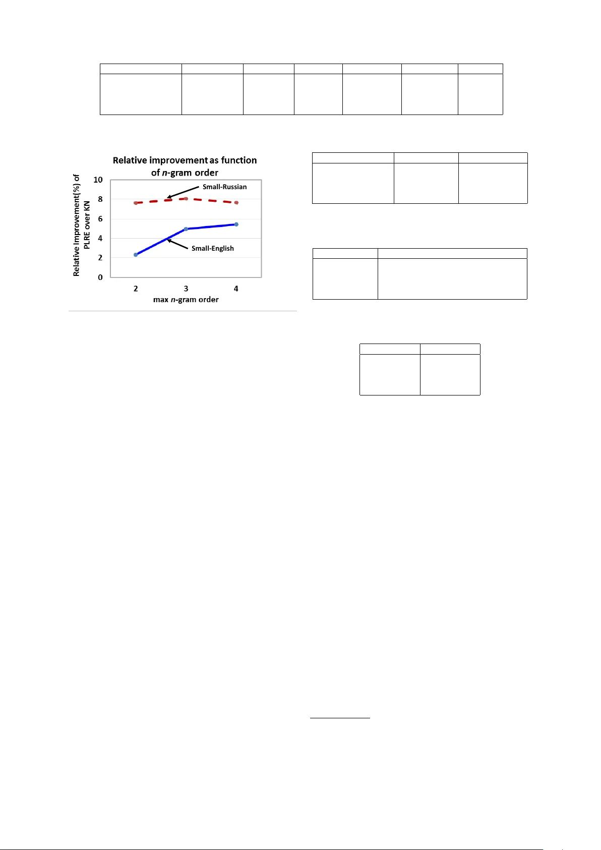
Language Modeling with P ower Lo w Rank Ensembles Ankur P . Parikh School of Computer Science Carnegie Mellon Uni v ersity apparikh@cs.cmu.edu A vneesh Saluja Electrical & Computer Engineering Carnegie Mellon Uni v ersity avneesh@cs.cmu.edu Chris Dyer School of Computer Science Carnegie Mellon Uni v ersity cdyer@cs.cmu.edu Eric P . Xing School of Computer Science Carnegie Mellon Uni v ersity epxing@cs.cmu.edu Abstract W e present po wer low rank ensembles (PLRE), a fle xible frame w ork for n -gram language modeling where ensembles of lo w rank matrices and tensors are used to obtain smoothed probability estimates of words in context. Our method can be understood as a generalization of n - gram modeling to non-integer n , and in- cludes standard techniques such as abso- lute discounting and Kneser-Ne y smooth- ing as special cases. PLRE training is effi- cient and our approach outperforms state- of-the-art modified Kneser Ney baselines in terms of perplexity on large corpora as well as on BLEU score in a downstream machine translation task. 1 Intr oduction Language modeling is the task of estimating the probability of sequences of words in a language and is an important component in, among other applications, automatic speech recognition (Ra- biner and Juang, 1993) and machine translation (K oehn, 2010). The predominant approach to lan- guage modeling is the n -gram model, wherein the probability of a word sequence P ( w 1 , . . . , w ` ) is decomposed using the chain rule, and then a Marko v assumption is made: P ( w 1 , . . . , w ` ) ≈ Q ` i =1 P ( w i | w i − 1 i − n +1 ) . While this assumption sub- stantially reduces the modeling complexity , pa- rameter estimation remains a major challenge. Due to the po wer -la w nature of language (Zipf, 1949), the maximum likelihood estimator mas- si vely overestimates the probability of rare ev ents and assigns zero probability to le gitimate word se- quences that happen not to ha ve been observed in the training data (Manning and Sch ¨ utze, 1999). Many smoothing techniques have been pro- posed to address the estimation challenge. These reassign probability mass (generally from over - estimated e vents) to unseen w ord sequences, whose probabilities are estimated by interpolating with or backing off to lo wer order n -gram models (Chen and Goodman, 1999). Some what surprisingly , these widely used smoothing techniques dif fer substantially from techniques for coping with data sparsity in other domains, such as collaborative filtering (Koren et al., 2009; Su and Khoshgoftaar , 2009) or matrix completion (Cand ` es and Recht, 2009; Cai et al., 2010). In these areas, low rank approaches based on matrix factorization play a central role (Lee and Seung, 2001; Salakhutdinov and Mnih, 2008; Macke y et al., 2011). For example, in recom- mender systems, a key challenge is dealing with the sparsity of ratings from a single user , since typical users will have rated only a few items. By projecting the lo w rank representation of a user’ s (sparse) preferences into the original space, an es- timate of ratings for new items is obtained. These methods are attractive due to their computational ef ficiency and mathematical well-foundedness. In this paper , we introduce power low rank en- sembles (PLRE), in which low rank tensors are used to produce smoothed estimates for n -gram probabilities. Ideally , we would like the low rank structures to discov er semantic and syntactic relat- edness among words and n -grams, which are used to produce smoothed estimates for word sequence probabilities. In contrast to the few previous low rank language modeling approaches, PLRE is not orthogonal to n -gram models, but rather a gen- eral framework where existing n -gram smoothing methods such as Kneser-Ney smoothing are spe- cial cases. A key insight is that PLRE does not compute low rank approximations of the original joint count matrices (in the case of bigrams) or ten- sors i.e. multi-way arrays (in the case of 3-grams and above), but instead altered quantities of these counts based on an element-wise power operation, similar to how some smoothing methods modify their lo wer order distributions. Moreov er , PLRE has two ke y aspects that lead to easy scalability for large corpora and vocab u- laries. First, since it utilizes the original n -grams, the ranks required for the lo w rank matrices and tensors tend to be remain tractable (e.g. around 100 for a v ocabulary size V ≈ 1 × 10 6 ) leading to fast training times. This differentiates our ap- proach ov er other methods that le verage an under- lying latent space such as neural networks (Bengio et al., 2003; Mnih and Hinton, 2007; Mikolov et al., 2010) or soft-class models (Saul and Pereira, 1997) where the underlying dimension is required to be quite large to obtain good performance. Moreov er , at test time, the probability of a se- quence can be queried in time O ( κ max ) where κ max is the maximum rank of the low rank matri- ces/tensors used. While this is larger than Kneser Ney’ s virtually constant query time, it is substan- tially faster than conditional e xponential family models (Chen and Rosenfeld, 2000; Chen, 2009; Nelakanti et al., 2013) and neural networks which require O ( V ) for e xact computation of the nor- malization constant. See Section 7 for a more de- tailed discussion of related work. Outline: W e first revie w existing n -gram smoothing methods ( § 2) and then present the in- tuition behind the key components of our tech- nique: rank ( § 3.1) and power ( § 3.2). W e then sho w how these can be interpolated into an ensem- ble ( § 4). In the experimental ev aluation on English and Russian corpora ( § 5), we find that PLRE out- performs Kneser-Ne y smoothing and all its vari- ants, as well as class-based language models. W e also include a comparison to the log-bilinear neu- ral language model (Mnih and Hinton, 2007) and e v aluate performance on a do wnstream machine translation task ( § 6) where our method achie ves consistent improv ements in BLEU. 2 Discount-based Smoothing W e first provide background on absolute discount- ing (Ney et al., 1994) and Kneser-Ney smooth- ing (Kneser and Ne y , 1995), two common n -gram smoothing methods. Both methods can be formu- lated as back-off or interpolated models; we de- scribe the latter here since that is the basis of our lo w rank approach. 2.1 Notation Let c ( w ) be the count of word w , and similarly c ( w , w i − 1 ) for the joint count of words w and w i − 1 . For shorthand we will define w j i to denote the word sequence { w i , w i +1 , ..., w j − 1 , w j } . Let b P ( w i ) refer to the maximum likelihood estimate (MLE) of the probability of word w i , and simi- larly b P ( w i | w i − 1 ) for the probability conditioned on a history , or more generally , b P ( w i | w i − 1 i − n +1 ) . Let N − ( w i ) := |{ w : c ( w i , w ) > 0 }| be the number of distinct words that appear be- fore w i . More generally , let N − ( w i i − n +1 ) = |{ w : c ( w i i − n +1 , w ) > 0 }| . Similarly , let N + ( w i − 1 i − n +1 ) = |{ w : c ( w, w i − 1 i − n +1 ) > 0 }| . V denotes the vocab ulary size. 2.2 Absolute Discounting Absolute discounting works on the idea of inter- polating higher order n -gram models with lower - order n -gram models. Howe ver , first some prob- ability mass must be “subtracted” from the higher order n -grams so that the leftover probability can be allocated to the lower order n -grams. More specifically , define the following discounted con- ditional probability: b P D ( w i | w i − 1 i − n +1 ) = max { c ( w i , w i − 1 i − n +1 ) − D , 0 } c ( w i − 1 i − n +1 ) Then absolute discounting P abs ( · ) uses the follow- ing (recursi ve) equation: P abs ( w i | w i − 1 i − n +1 ) = b P D ( w i | w i − 1 i − n +1 ) + γ ( w i − 1 i − n +1 ) P abs ( w i | w i − 1 i − n +2 ) where γ ( w i − 1 i − n +1 ) is the lefto ver weight (due to the discounting) that is chosen so that the con- ditional distribution sums to one: γ ( w i − 1 i − n +1 ) = D c ( w i − 1 i − n +1 ) N + ( w i − 1 i − n +1 ) . F or the base case, we set P abs ( w i ) = b P ( w i ) . Discontinuity: Note that if c ( w i − 1 i − n +1 ) = 0 , then γ ( w i − 1 i − n +1 ) = 0 0 , in which case γ ( w i − 1 i − n +1 ) is set to 1. W e will see that this discontinuity appears in PLRE as well. 2.3 Kneser Ney Smoothing Ideally , the smoothed probability should preserve the observed unigram distrib ution: b P ( w i ) = X w i − 1 i − n +1 P sm ( w i | w i − 1 i − n +1 ) b P ( w i − 1 i − n +1 ) (1) where P sm ( w i | w i − 1 i − n +1 ) is the smoothed condi- tional probability that a model outputs. Unfortu- nately , absolute discounting does not satisfy this property , since it exclusi vely uses the unaltered MLE unigram model as its lower order model. In practice, the lower order distribution is only uti- lized when we are unsure about the higher order distribution (i.e., when γ ( · ) is large). Therefore, the unigram model should be altered to condition on this fact. This is the inspiration behind Kneser -Ney (KN) smoothing, an elegant algorithm with robust per- formance in n -gram language modeling. KN smoothing defines alternate probabilities P alt ( · ) : P alt D ( w i | w i − 1 i − n 0 +1 ) =        b P D ( w i | w i − 1 i − n 0 +1 ) , if n 0 = n max { N − ( w i i − n 0 +1 ) − D, 0 } P w i N − ( w i i − n 0 +1 ) , if n 0 < n The base case for unigrams reduces to P alt ( w i ) = N − ( w i ) P w i N − ( w i ) . Intuiti vely P alt ( w i ) is proportional to the number of unique words that precede w i . Thus, words that appear in many dif- ferent contexts will be giv en higher weight than words that consistently appear after only a fe w contexts. These alternate distributions are then used with absolute discounting: P kn ( w i | w i − 1 i − n +1 ) = P alt D ( w i | w i − 1 i − n +1 ) + γ ( w i − 1 i − n +1 ) P kn ( w i | w i − 1 i − n +2 ) (2) where we set P kn ( w i ) = P alt ( w i ) . By definition, KN smoothing satisfies the marginal constraint in Eq. 1 (Kneser and Ney , 1995). 3 Po wer Low Rank Ensembles In n -gram smoothing methods, if a bigram count c ( w i , w i − 1 ) is zero, the unigram probabilities are used, which is equiv alent to assuming that w i and w i − 1 are independent ( and similarly for general n ). Ho we ver , in this situation, instead of back- ing off to a 1 -gram, we may like to back off to a “ 1 . 5 -gram” or more generally an order between 1 and 2 that captures a coarser le vel of dependence between w i and w i − 1 and does not assume full in- dependence. Inspired by this intuition, our strategy is to con- struct an ensemble of matrices and tensors that not only consists of MLE-based count informa- tion, but also contains quantities that represent lev- els of dependence in-between the v arious orders in the model. W e call these combinations power lo w rank ensembles (PLRE), and they can be thought of as n -gram models with non-integer n . Our ap- proach can be recursi vely formulated as: P plre ( w i | w i − 1 i − n +1 ) = P alt D 0 ( w i | w i − 1 i − n +1 ) + γ 0 ( w i − 1 i − n +1 )  Z D 1 ( w i | w i − 1 i − n +1 ) + ..... + γ η − 1 ( w i − 1 i − n +1 )  Z D η ( w i | w i − 1 i − n +1 ) + γ η ( w i − 1 i − n +1 )  P plre ( w i | w i − 1 i − n +2 )  ...  (3) where Z 1 , ..., Z η are conditional probability ma- trices that represent the intermediate n -gram or- ders 1 and D is a discount function (specified in § 4). This formulation begs answers to a fe w crit- ical questions. Ho w to construct matrices that represent conditional probabilities for intermedi- ate n ? Ho w to transform them in a way that generalizes the altered lower order distributions in KN smoothing? Ho w to combine these matri- ces such that the marginal constraint in Eq. 1 still holds? The following propose solutions to these three queries: 1. Rank (Section 3.1): Rank gi ves us a concrete measurement of the dependence between w i and w i − 1 . By constructing lo w rank ap- proximations of the bigram count matrix and higher-order count tensors, we obtain matri- ces that represent coarser dependencies, with a rank one approximation implying that the v ariables are independent. 2. Power (Section 3.2): In KN smoothing, the lo wer order distributions are not the original counts but rather altered estimates. W e pro- pose a continuous generalization of this alter- ation by taking the element-wise power of the counts. 1 with a slight abuse of notation, let Z D j be shorthand for Z j, D j 3. Creating the Ensemble (Section 4): Lastly , PLRE also defines a way to interpolate the specifically constructed intermediate n -gram matrices. Unfortunately a constant discount, as presented in Section 2, will not in general preserve the lower order marginal constraint (Eq. 1). W e propose a generalized discount- ing scheme to ensure the constraint holds. 3.1 Rank W e first show ho w rank can be utilized to construct quantities between an n -gram and an n − 1 -gram. In general, we think of an n -gram as an n th or- der tensor i.e. a multi-way array with n indices { i 1 , ..., i n } . (A vector is a tensor of order 1, a ma- trix is a tensor of order 2 etc.) Computing a spe- cial rank one approximation of slices of this tensor produces the n − 1 -gram. Thus, taking rank κ ap- proximations in this fashion allo ws us to represent dependencies between an n -gram and n − 1 -gram. Consider the bigram count matrix B with N counts which has rank V . Note that b P ( w i | w i − 1 ) = B ( w i ,w i − 1 ) P w B ( w,w i − 1 ) . Additionally , B can be considered a random variable that is the re- sult of sampling N tuples of ( w i , w i − 1 ) and ag- glomerating them into a count matrix. Assum- ing w i and w i − 1 are independent, the e xpected v alue (with respect to the empirical distribution) E [ B ] = N P ( w i ) P ( w i − 1 ) , which can be rewrit- ten as being proportional to the outer product of the unigram probability vector with itself, and is thus rank one. This observation e xtends to higher order n -grams as well. Let C n be the n th order tensor where C n ( w i , ...., w i − n +1 ) = c ( w i , ..., w i − n +1 ) . Furthermore denote C n (: , ˜ w i − 1 i − n +2 , :) to be the V × V matrix slice of C n where w i − n +2 , ..., w i − 1 are held fix ed to a particular sequence ˜ w i − n +2 , ..., ˜ w i − 1 . Then if w i is con- ditionally independent of w i − n +1 gi ven w i − 1 i − n +2 , then E [ C n (: , ˜ w i − 1 i − n +2 , :)] is rank one ∀ ˜ w i − 1 i − n +2 . Ho we ver , it is rare that these matrices are ac- tually rank one, either due to sampling vari- ance or the fact that w i and w i − 1 are not in- dependent. What we would really like to say is that the best rank one approximation B (1) (under some norm) of B is ∝ b P ( w i ) b P ( w i − 1 ) . While this statement is not true under the ` 2 norm, it is true under generalized KL diver - gence (Lee and Seung, 2001): g K L ( A || B ) = P ij  A ij log( A ij B ij ) − A ij + B ij )  . In particular , generalized KL div ergence pre- serves row and column sums: if M ( κ ) is the best rank κ appr oximation of M under g K L then the r ow sums and column sums of M ( κ ) and M ar e equal (Ho and V an Dooren, 2008). Leveraging this property , it is straightforward to pro ve the fol- lo wing lemma: Lemma 1. Let B ( κ ) be the best rank κ ap- pr oximation of B under gKL. Then B (1) ∝ b P ( w i ) b P ( w i − 1 ) and ∀ w i − 1 s.t. c ( w i − 1 ) 6 = 0 : b P ( w i ) = B (1) ( w i , w i − 1 ) P w B (1) ( w , w i − 1 ) F or mor e gener al n , let C n, ( κ ) i − 1 ,...,i − n +2 be the best rank κ appr oximation of C n (: , ˜ w i − 1 i − n +2 , : ) under g K L . Then similarly , ∀ w i − 1 i − n +1 s.t. c ( w i − 1 i − n +1 ) > 0 : b P ( w i | w i − 1 , ..., w i − n +2 ) = C n, (1) i − 1 ,...,i − n +2 ( w i , w i − 1 i − n +1 ) P w C n, (1) i − 1 ,...,i − n +2 ( w , w i − 1 i − n +1 ) (4) Thus, by selecting 1 < κ < V , we obtain count matrices and tensors between n and n − 1 -grams. The condition that c ( w i − 1 i − n +1 ) > 0 corresponds to the discontinuity discussed in § 2.2. 3.2 Po wer Since KN smoothing alters the lower order distri- butions instead of simply using the MLE, vary- ing the rank is not sufficient in order to generalize this suite of techniques. Thus, PLRE computes lo w rank approximations of altered count matri- ces. Consider taking the elementwise power ρ of the bigram count matrix, which is denoted by B · ρ . For example, the observed bigram count matrix and associated ro w sum: B · 1 = 1 . 0 2 . 0 1 . 0 0 5 . 0 0 2 . 0 0 0 ! row sum → 4 . 0 5 . 0 2 . 0 ! As expected the ro w sum is equal to the uni- gram counts (which we denote as u ). Now con- sider B · 0 . 5 : B · 0 . 5 = 1 . 0 1 . 4 1 . 0 0 2 . 2 0 1 . 4 0 0 ! row sum → 3 . 4 2 . 2 1 . 4 ! Note how the row sum vector has been altered. In particular since w 1 (corresponding to the first ro w) has a more div erse history than w 2 , it has a higher row sum (compared to in u where w 2 has the higher row sum). Lastly , consider the case when p = 0 : B · 0 = 1 . 0 1 . 0 1 . 0 0 1 . 0 0 1 . 0 0 0 ! row sum → 3 . 0 1 . 0 1 . 0 ! The row sum is now the number of unique words that precede w i (since B 0 is binary) and is thus equal to the (unnormalized) Kneser Ney unigram. This idea also generalizes to higher order n -grams and leads us to the follo wing lemma: Lemma 2. Let B ( ρ,κ ) be the best rank κ ap- pr oximation of B · ρ under gKL. Then ∀ w i − 1 s.t. c ( w i − 1 ) 6 = 0 : P alt ( w i ) = B (0 , 1) ( w i , w i − 1 ) P w B (0 , 1) ( w , w i − 1 ) F or more general n , let C n, ( ρ,κ ) i − 1 ,...,i − n +2 be the best rank κ appr oximation of C n, ( ρ ) (: , ˜ w i − 1 i − n +2 , :) un- der g K L . Similarly , ∀ w i − 1 i − n +1 s.t. c ( w i − 1 i − n +1 ) > 0 : P alt ( w i | w i − 1 , ..., w i − n +2 ) = C n, (0 , 1) i − 1 ,...,i − n +2 ( w i , w i − 1 i − n +1 ) P w C n, (0 , 1) i − 1 ,...,i − n +2 ( w , w i − 1 i − n +1 ) (5) 4 Creating the Ensemble Recall our ov erall formulation in Eq. 3; a naiv e solution would be to set Z 1 , ..., Z η to low rank approximations of the count matrices/tensors un- der varying powers, and then interpolate through constant absolute discounting. Unfortunately , the marginal constraint in Eq. 1 will generally not hold if this strategy is used. Therefore, we propose a generalized discounting scheme where each non- zero n -gram count is associated with a different discount D j ( w i , w i − 1 i − n 0 +1 ) . The lo w rank approxi- mations are then computed on the discounted ma- trices, leaving the mar ginal constraint intact. For clarity of exposition, we focus on the spe- cial case where n = 2 with only one low rank matrix before stating our general algorithm: P plre ( w i | w i − 1 ) = b P D 0 ( w i | w i − 1 ) + γ 0 ( w i − 1 )  Z D 1 ( w i | w i − 1 ) + γ 1 ( w i − 1 ) P alt ( w i )  (6) Our goal is to compute D 0 , D 1 and Z 1 so that the follo wing lower order marginal constraint holds: b P ( w i ) = X w i − 1 P plre ( w i | w i − 1 ) b P ( w i − 1 ) (7) Our solution can be thought of as a two- step procedure where we compute the discounts D 0 , D 1 (and the γ ( w i − 1 ) weights as a by- product), follo wed by the low rank quantity Z 1 . First, we construct the following intermediate en- semble of po wered, but full rank terms. Let Y ρ j be the matrix such that Y ρ j ( w i , w i − 1 ) := c ( w i , w i − 1 ) ρ j . Then define P pwr ( w i | w i − 1 ) := Y ( ρ 0 =1) D 0 ( w i | w i − 1 ) + γ 0 ( w i − 1 )  Y ( ρ 1 ) D 1 ( w i | w i − 1 ) + γ 1 ( w i − 1 ) Y ( ρ 2 =0) ( w i | w i − 1 )  (8) where with a little abuse of notation: Y ρ j D j ( w i | w i − 1 ) = c ( w i , w i − 1 ) ρ j − D j ( w i , w i − 1 ) P w i c ( w i , w i − 1 ) ρ j Note that P alt ( w i ) has been replaced with Y ( ρ 2 =0) ( w i | w i − 1 ) , based on Lemma 2, and will equal P alt ( w i ) once the lo w rank approximation is taken as discussed in § 4.2). Since we hav e only combined terms of differ - ent po wer (but all full rank), it is natural choose the discounts so that the result remains unchanged i.e., P pwr ( w i | w i − 1 ) = b P ( w i | w i − 1 ) , since the low rank approximation (not the po wer) will imple- ment smoothing. Enforcing this constraint giv es rise to a set of linear equations that can be solved (in closed form) to obtain the discounts as we now sho w belo w . 4.1 Step 1: Computing the Discounts T o ensure the constraint that P pwr ( w i | w i − 1 ) = b P ( w i | w i − 1 ) , it is sufficient to enforce the follow- ing two local constraints: Y ( ρ j ) ( w i | w i − 1 ) = Y ( ρ j ) D j ( w i | w i − 1 ) + γ j ( w i − 1 ) Y ( ρ j +1 ) ( w i | w i − 1 ) for j = 0 , 1 (9) This allo ws each D j to be solv ed for indepen- dently of the other { D j 0 } j 0 6 = j . Let c i,i − 1 = c ( w i , w i − 1 ) , c j i,i − 1 = c ( w i , w i − 1 ) ρ j , and d j i,i − 1 = D j ( w i , w i − 1 ) . Expanding Eq. 9 yields that ∀ w i , w i − 1 : c j i,i − 1 P i c j i,i − 1 = c j i,i − 1 − d j i,i − 1 P i c j i,i − 1 + P i d j i,i − 1 P i c j i,i − 1 ! c j +1 i,i − 1 P i c j +1 i,i − 1 (10) which can be re written as: − d j i,i − 1 + X i d j i,i − 1 ! c j +1 i,i − 1 P i c j +1 i,i − 1 = 0 (11) Note that Eq. 11 decouples across w i − 1 since the only d j i,i − 1 terms that are dependent are the ones that share the preceding context w i − 1 . It is straightforw ard to see that setting d j i,i − 1 proportional to c j +1 i,i − 1 satisfies Eq. 11. Furthermore it can be shown that all solutions are of this form (i.e., the linear system has a null space of exactly one). Moreo ver , we are interested in a particular subset of solutions where a single parameter d ∗ (independent of w i − 1 ) controls the scaling as in- dicated by the follo wing lemma: Lemma 3. Assume that ρ j ≥ ρ j +1 . Choose any 0 ≤ d ∗ ≤ 1 . Set d j i,i − 1 = d ∗ c j +1 i,i − 1 ∀ i, j . The r esulting discounts satisfy Eq. 11 as well as the inequality constraints 0 ≤ d j i,i − 1 ≤ c j i,i − 1 . Fur - thermor e, the leftover weight γ j takes the form: γ j ( w i − 1 ) = P i d j i,i − 1 P i c j i,i − 1 = d ∗ P i c j +1 i,i − 1 P i c j i,i − 1 Pr oof. Clearly this choice of d j i,i − 1 satisfies Eq. 11. The largest possible value of d j i,i − 1 is c j +1 i,i − 1 . ρ j ≥ ρ j +1 , implies c j i,i − 1 ≥ c j +1 i,i − 1 . Thus the inequality constraints are met. It is then easy to verify that γ takes the abov e form. The above lemma generalizes to longer contexts (i.e. n > 2 ) as shown in Algorithm 1. Note that if ρ j = ρ j +1 then Algorithm 1 is equi v alent to scal- ing the counts e.g. deleted-interpolation/Jelinek Mercer smoothing (Jelinek and Mercer , 1980). On the other hand, when ρ j +1 = 0 , Algorithm 1 is equal to the absolute discounting that is used in Kneser-Ney . Thus, depending on ρ j +1 , our method generalizes different types of interpola- tion schemes to construct an ensemble so that the marginal constraint is satisfied. Algorithm 1 Compute D In : Count tensor C n , powers ρ j , ρ j +1 such that ρ j ≥ ρ j +1 , and parameter d ∗ . Out : Discount D j for powered counts C n, ( ρ j ) and associated leftov er weight γ j 1: Set D j ( w i , w i − 1 i − n +1 ) = d ∗ c ( w i , w i − 1 i − n +1 ) ρ j +1 . 2: γ j ( w i , w i − 1 i − n +1 ) = d ∗ P w i c ( w i , w i − 1 i − n +1 ) ρ j +1 P w i c ( w i , w i − 1 i − n +1 ) ρ j Algorithm 2 Compute Z In : Count tensor C n , power ρ , discounts D , rank κ Out : Discounted low rank conditional probability table Z ( ρ,κ ) D ( w i | w i − 1 i − n +1 ) (represented implicitly) 1: Compute powered counts C n, ( · ρ ) . 2: Compute denominators P w i c ( w i , w i − 1 i − n +1 ) ρ ∀ w i − 1 i − n +1 s.t. c ( w i − 1 i − n +1 ) > 0 . 3: Compute discounted po wered counts C n, ( · ρ ) D = C n, ( · ρ ) − D . 4: For each slice M ˜ w i − 1 i − n +2 := C n, ( · ρ ) D (: , ˜ w i − 1 i − n +2 , :) compute M ( κ ) := min A ≥ 0: rank ( A )= κ k M ˜ w i − 1 i − n +2 − A k K L (stored implicitly as M ( κ ) = LR ) Set Z ( ρ,κ ) D (: , ˜ w i − 1 i − n +2 , :) = M ( κ ) 5: Note that Z ( ρ,κ ) D ( w i | w i − 1 i − n +1 ) = Z ( ρ,κ ) D ( w i , w i − 1 i − n +1 ) P w i c ( w i , w i − 1 i − n +1 ) ρ 4.2 Step 2: Computing Low Rank Quantities The next step is to compute low rank approxi- mations of Y ( ρ j ) D j to obtain Z D j such that the inter- mediate marginal constraint in Eq. 7 is preserved. This constraint trivially holds for the intermediate ensemble P pwr ( w i | w i − 1 ) due to ho w the discounts were deriv ed in § 4.1. For our running bigram ex- ample, define Z ( ρ j ,κ j ) D j to be the best rank κ j ap- proximation to Y ( ρ j ,κ j ) D j according to g K L and let Z ρ j ,κ j D j ( w i | w i − 1 ) = Z ρ j ,κ j D j ( w i , w i − 1 ) P w i c ( w i , w i − 1 ) ρ j Note that Z ρ j ,κ j D j ( w i | w i − 1 ) is a valid (discounted) conditional probability since g K L preserves ro w/column sums so the denominator remains un- changed under the low rank approximation. Then using the fact that Z (0 , 1) ( w i | w i − 1 ) = P alt ( w i ) (Lemma 2) we can embellish Eq. 6 as P plre ( w i | w i − 1 ) = P D 0 ( w i | w i − 1 )+ γ 0 ( w i − 1 )  Z ( ρ 1 ,κ 1 ) D 1 ( w i | w i − 1 ) + γ 1 ( w i − 1 ) P alt ( w i )  Le veraging the form of the discounts and ro w/column sum preserving property of g K L , we then hav e the following lemma (the proof is in the supplementary material): Lemma 4. Let P plr e ( w i | w i − 1 ) indicate the PLRE smoothed conditional pr obability as computed by Eq. 6 and Algorithms 1 and 2. Then, the marginal constraint in Eq. 7 holds. 4.3 More general algorithm In general, the principles outlined in the pre vi- ous sections hold for higher order n -grams. As- sume that the discounts are computed according to Algorithm 1 with parameter d ∗ and Z ( ρ j ,κ j ) D j is computed according to Algorithm 2. Note that, as sho wn in Algorithm 2, for higher order n -grams, the Z ( ρ j ,κ j ) D j are created by taking lo w rank approx- imations of slices of the (powered) count tensors (see Lemma 2 for intuition). Eq. 3 can now be embellished: P plre ( w i | w i − 1 i − n +1 ) = P alt D 0 ( w i | w i − 1 i − n +1 ) + γ 0 ( w i − 1 i − n +1 )  Z ( ρ 1 ,κ 1 ) D 1 ( w i | w i − 1 i − n +1 ) + ..... + γ η − 1 ( w i − 1 i − n +1 )  Z ( ρ η ,κ η ) D η ( w i | w i − 1 i − n +1 ) + γ η ( w i − 1 i − n +1 )  P plre ( w i | w i − 1 i − n +2 )  ...  (12) Lemma 4 also applies in this case and is giv en in Theorem 1 in the supplementary material. 4.4 Links with KN Smoothing In this section, we explicitly show the relation- ship between PLRE and KN smoothing. Re writ- ing Eq. 12 in the follo wing form: P plre ( w i | w i − 1 i − n +1 ) = P terms plre ( w i | w i − 1 i − n +1 ) + γ 0: η ( w i − 1 i − n +1 ) P plre ( w i | w i − 1 i − n +2 ) (13) where P terms plre ( w i | w i − 1 i − n +1 ) contains the terms in Eq. 12 except the last, and γ 0: η ( w i − 1 i − n +1 ) = Q η h =0 γ h ( w i − 1 i − n +1 ) , we can lev erage the form of the discount, and using the fact that ρ η +1 = 0 2 : γ 0: η ( w i − 1 i − n − 1 ) = d ∗ η +1 N + ( w i − 1 i − n +1 ) c ( w i − 1 i − n +1 ) W ith this form of γ ( · ) , Eq. 13 is remarkably sim- ilar to KN smoothing (Eq. 2) if KN’ s discount pa- rameter D is chosen to equal ( d ∗ ) η +1 . The difference is that P alt ( · ) has been replaced with the alternate estimate P terms plre ( w i | w i − 1 i − n +1 ) , which hav e been enriched via the low rank struc- ture. Since these alternate estimates were con- structed via our ensemble strate gy they contain both very fine-grained dependencies (the origi- nal n -grams) as well as coarser dependencies (the lo wer rank n -grams) and is thus fundamentally dif ferent than simply taking a single matrix/tensor decomposition of the trigram/bigram matrices. Moreov er , it provides a natural way of setting d ∗ based on the Good-T uring (GT) estimates em- ployed by KN smoothing. In particular , we can set d ∗ to be the ( η + 1) th root of the KN discount D that can be estimated via the GT estimates. 4.5 Computational Considerations PLRE scales well even as the order n increases. T o compute a low rank bigram, one low rank ap- proximation of a V × V matrix is required. For the low rank trigram, we need to compute a low rank approximation of each slice C n, ( · p ) D (: , ˜ w i − 1 , : ) ∀ ˜ w i − 1 . While this may seem daunting at first, in practice the size of each slice (number of non-zero ro ws/columns) is usually much, much smaller than V , keeping the computation tractable. Similarly , PLRE also ev aluates conditional probabilities at e v aluation time ef ficiently . As sho wn in Algorithm 2, the normalizer can be pre- computed on the sparse powered matrix/tensor . As a result our test complexity is O ( P η total i =1 κ i ) where η total is the total number of matrices/tensors in the ensemble. While this is lar ger than Kneser Ney’ s practically constant complexity of O ( n ) , it is much faster than other recent methods for language modeling such as neural networks and conditional exponential family models where ex- act computation of the normalizing constant costs O ( V ) . 5 Experiments T o ev aluate PLRE, we compared its performance on English and Russian corpora with sev eral vari- 2 for derivation see proof of Lemma 4 in the supplemen- tary material ants of KN smoothing, class-based models, and the log-bilinear neural language model (Mnih and Hinton, 2007). W e ev aluated with perplexity in most of our experiments, but also provide results e v aluated with BLEU (Papineni et al., 2002) on a do wnstream machine translation (MT) task. W e hav e made the code for our approach publicly av ailable 3 . T o build the hard class-based LMs, we utilized mkcls 4 , a tool to train word classes that uses the maximum likelihood criterion (Och, 1995) for classing. W e subsequently trained trigram class language models on these classes (correspond- ing to 2 nd -order HMMs) using SRILM (Stolcke, 2002), with KN-smoothing for the class transition probabilities. SRILM was also used for the base- line KN-smoothed models. For our MT ev aluation, we built a hierarchi- cal phrase translation (Chiang, 2007) system us- ing cdec (Dyer et al., 2010). The KN-smoothed models in the MT experiments were compiled us- ing K enLM (Heafield, 2011). 5.1 Datasets For the perplexity experiments, we ev aluated our proposed approach on 4 datasets, 2 in English and 2 in Russian. In all cases, the singletons were re- placed with “ < unk > ” tokens in the training cor- pus, and any word not in the vocab ulary was re- placed with this token during ev aluation. There is a general dearth of ev aluation on large-scale cor- pora in morphologically rich languages such as Russian, and thus we ha ve made the processed Large-Russian corpus a vailable for comparison 3 . • Small-English : APNews corpus (Bengio et al., 2003): T rain - 14 million words, De v - 963,000, T est - 963,000. V ocabulary- 18,000 types. • Small-Russian : Subset of Russian news com- mentary data from 2013 WMT translation task 5 : T rain- 3.5 million words, Dev - 400,000 T est - 400,000. V ocabulary - 77,000 types. • Large-English : English Gigaword, T raining - 837 million words, Dev - 8.7 million, T est - 8.7 million. V ocabulary- 836,980 types. • Large-Russian : Monolingual data from WMT 2013 task. T raining - 521 million words, V ali- dation - 50,000, T est - 50,000. V ocab ulary- 1.3 million types. 3 http://www .cs.cmu.edu/ ∼ apparikh/plre.html 4 http://code.google.com/p/giza-pp/ 5 http://www .statmt.org/wmt13/training-monolingual- nc-v8.tgz For the MT e valuation, we used the parallel data from the WMT 2013 shared task, excluding the Common Crawl corpus data. The ne wstest2012 and ne wstest2013 ev aluation sets were used as the de velopment and test sets respecti vely . 5.2 Small Corpora For the class-based baseline LMs, the number of classes was selected from { 32 , 64 , 128 , 256 , 512 , 1024 } (Small-English) and { 512 , 1024 } (Small-Russian). W e could not go higher due to the computationally laborious process of hard clustering. For Kneser-Ne y , we explore four dif ferent variants: back-off (BO-KN) interpolated (int-KN), modified back-off (BO- MKN), and modified interpolated (int-MKN). Good-T uring estimates were used for discounts. All models trained on the small corpora are of order 3 (trigrams). For PLRE, we used one low rank bigram and one low rank trigram in addition to the MLE n - gram estimates. The powers of the intermediate matrices/tensors were fixed to be 0 . 5 and the dis- counts were set to be square roots of the Good T ur- ing estimates (as explained in § 4.4). The ranks were tuned on the dev elopment set. For Small- English, the ranges were { 1 e − 3 , 5 e − 3 } (as a fraction of the vocab ulary size) for both the low rank bigram and low rank trigram models. F or Small-Russian the ranges were { 5 e − 4 , 1 e − 3 } for both the low rank bigram and the low rank tri- gram models. The results are shown in T able 1. The best class- based LM is reported, but is not competitiv e with the KN baselines. PLRE outperforms all of the baselines comfortably . Moreover , PLRE’ s perfor- mance ov er the baselines is highlighted in Russian. W ith larger vocab ulary sizes, the lo w rank ap- proach is more ef fecti ve as it can capture linguistic similarities between rare and common words. Next we discuss how the maximum n -gram or- der affects performance. Figure 1 shows the rela- ti ve percentage impro vement of our approach o ver int-MKN as the order is increased from 2 to 4 for both methods. The Small-English dataset has a rather small vocabulary compared to the number of tokens, leading to lower data sparsity in the bi- gram. Thus the PLRE improv ement is small for order = 2 , but more substantial for order = 3 . On the other hand, for the Small-Russian dataset, the vocab ulary size is much larger and consequently the bigram counts are sparser . This leads to sim- Dataset class-1024(3) BO-KN(3) int-KN(3) BO-MKN(3) int-MKN(3) PLRE(3) Small-English Dev 115.64 99.20 99.73 99.95 95.63 91.18 Small-English T est 119.70 103.86 104.56 104.55 100.07 95.15 Small-Russian Dev 286.38 281.29 265.71 287.19 263.25 241.66 Small-Russian T est 284.09 277.74 262.02 283.70 260.19 238.96 T able 1: Perplexity results on small corpora for all methods. Sm al l - Rus si an Sm al l - Eng li sh Figure 1: Relati ve percentage improv ement of PLRE over int-MKN as the maximum n -gram or- der for both methods is increased. ilar improvements for all orders (which are larger than that for Small-English). On both these datasets, we also experimented with tuning the discounts for int-MKN to see if the baseline could be improved with more careful choices of discounts. Howe ver , this achieved only marginal gains (reducing the perplexity to 98 . 94 on the Small-English test set and 259 . 0 on the Small-Russian test set). Comparison to LBL (Mnih and Hinton, 2007) : Mnih and Hinton (2007) ev aluate on the Small-English dataset (b ut remo ve end markers and concatenate the sentences). They obtain per- plexities 117 . 0 and 107 . 8 using contexts of size 5 and 10 respectiv ely . With this preprocessing, a 4- gram (context 3) PLRE achie ves 108 . 4 perplexity . 5.3 Large Corpora Results on the lar ger corpora for the top 2 per- forming methods “PLRE” and “int-MKN” are pre- sented in T able 2. Due to the larger training size, we use 4-gram models in these experiments. How- e ver , including the lo w rank 4-gram tensor pro- vided little gain and therefore, the 4-gram PLRE only has additional low rank bigram and low rank trigram matrices/tensors. As abov e, ranks were tuned on the de velopment set. For Large-English, the ranges were { 1 e − 4 , 5 e − 4 , 1 e − 3 } (as a frac- tion of the vocabulary size) for both the low rank Dataset int-MKN(4) PLRE(4) Large-English De v 73.21 71.21 Large-English T est 77.90 ± 0.203 75.66 ± 0.189 Large-Russian De v 326.9 297.11 Large-Russian T est 289.63 ± 6.82 264.59 ± 5.839 T able 2: Mean perplexity results on large corpora, with standard de viation. Dataset PLRE T raining T ime Small-English 3.96 min ( order 3) / 8.3 min (order 4) Small-Russian 4.0 min (order 3) / 4.75 min (order 4) Large-English 3.2 hrs (order 4) Large-Russian 8.3 hrs (order 4) T able 3: PLRE training times for a fixed parameter setting 6 . 8 Intel Xeon CPUs were used. Method BLEU int-MKN(4) 17.63 ± 0.11 PLRE(4) 17.79 ± 0.07 Smallest Diff PLRE+0.05 Largest Dif f PLRE+0.29 T able 4: Results on English-Russian translation task (mean ± stde v). See text for details. bigram and low rank trigram models. For Small- Russian the ranges were { 1 e − 5 , 5 e − 5 , 1 e − 4 } for both the low rank bigram and the low rank trigram models. For statistical v alidity , 10 test sets of size equal to the original test set were generated by ran- domly sampling sentences with replacement from the original test set. Our method outperforms “int- MKN” with gains similar to that on the smaller datasets. As sho wn in T able 3, our method obtains fast training times e ven for large datasets. 6 Machine T ranslation T ask T able 4 presents results for the MT task, trans- lating from English to Russian 7 . W e used MIRA (Chiang et al., 2008) to learn the feature weights. T o control for the randomness in MIRA, we av oid retuning when switching LMs - the set of feature weights obtained using int-MKN is the same, only the language model changes. The 6 As described earlier , only the ranks need to be tuned, so only 2-3 lo w rank bigrams and 2-3 lo w rank trigrams need to be computed (and combined depending on the setting). 7 the best score at WMT 2013 was 19.9 (Bojar et al., 2013) procedure is repeated 10 times to control for op- timizer instability (Clark et al., 2011). Unlike other recent approaches where an additional fea- ture weight is tuned for the proposed model and used in conjunction with KN smoothing (V aswani et al., 2013), our aim is to sho w the impro vements that PLRE pro vides as a substitute for KN. On a v- erage, PLRE outperforms the KN baseline by 0.16 BLEU, and this improvement is consistent in that PLRE ne ver gets a w orse BLEU score. 7 Related W ork Recent attempts to re visit the language model- ing problem hav e largely come from two direc- tions: Bayesian nonparametrics and neural net- works. T eh (2006) and Goldwater et al. (2006) discov ered the connection between interpolated Kneser Ney and the hierarchical Pitman-Y or pro- cess. These hav e led to generalizations that ac- count for domain effects (W ood and T eh, 2009) and unbounded contexts (W ood et al., 2009). The idea of using neural networks for language modeling is not ne w (Miikkulainen and Dyer , 1991), but recent efforts (Mnih and Hinton, 2007; Mikolo v et al., 2010) hav e achie ved impressi ve performance. These methods can be quite expen- si ve to train and query (especially as the vocab- ulary size increases). T echniques such as noise contrasti ve estimation (Gutmann and Hyv ¨ arinen, 2012; Mnih and T eh, 2012; V aswani et al., 2013), subsampling (Xu et al., 2011), or careful engi- neering approaches for maximum entropy LMs (which can also be applied to neural networks) (W u and Khudanpur , 2000) hav e improved train- ing of these models, b ut querying the probabil- ity of the next word given still requires explicitly normalizing ov er the vocab ulary , which is expen- si ve for big corpora or in languages with a large number of word types. Mnih and T eh (2012) and V aswani et al. (2013) propose setting the normal- ization constant to 1, but this is approximate and thus can only be used for downstream ev aluation, not for perplexity computation. An alternate tech- nique is to use word-classing (Goodman, 2001; Mikolo v et al., 2011), which can reduce the cost of e xact normalization to O ( √ V ) . In contrast, our approach is much more scalable, since it is triv- ially parallelized in training and does not require explicit normalization during e valuation. There are a few low rank approaches (Saul and Pereira, 1997; Belle garda, 2000; Hutchinson et al., 2011), but they are only effecti ve in restricted set- tings (e.g. small training sets, or corpora divided into documents) and do not generally perform comparably to state-of-the-art models. Roark et al. (2013) also use the idea of mar ginal constraints for re-estimating back-off parameters for heavily- pruned language models, whereas we use this con- cept to estimate n -gram specific discounts. 8 Conclusion W e presented power low rank ensembles, a tech- nique that generalizes existing n -gram smoothing techniques to non-integer n . By using ensembles of sparse as well as low rank matrices and ten- sors, our method captures both the fine-grained and coarse structures in word sequences. Our discounting strategy preserves the marginal con- straint and thus generalizes Kneser Ney , and un- der slight changes can also extend other smooth- ing methods such as deleted-interpolation/Jelinek- Mercer smoothing. Experimentally , PLRE con- vincingly outperforms Kneser-Ney smoothing as well as class-based baselines. Acknowledgements This work was supported by NSF IIS1218282, NSF IIS1218749, NSF IIS1111142, NIH R01GM093156, the U. S. Army Research Labo- ratory and the U. S. Army Research Office under contract/grant number W911NF-10-1-0533, the NSF Graduate Research Fellowship Program under Grant No. 0946825 (NSF Fellowship to APP), and a grant from Ebay Inc. (to AS). References Jerome R. Bellegarda. 2000. Large vocab ulary speech recognition with multispan statistical language mod- els. IEEE T ransactions on Speech and Audio Pro- cessing , 8(1):76–84. Y oshua Bengio, R ´ ejean Ducharme, Pascal V incent, and Christian Jan vin. 2003. A neural probabilistic lan- guage model. J. Mach. Learn. Res. , 3:1137–1155, March. Ond ˇ rej Bojar , Christian Buck, Chris Callison-Burch, Christian Federmann, Barry Haddow , Philipp K oehn, Christof Monz, Matt Post, Radu Soricut, and Lucia Specia. 2013. Findings of the 2013 W ork- shop on Statistical Machine Translation. In Pr o- ceedings of the Eighth W orkshop on Statistical Ma- chine T ranslation , pages 1–44, Sofia, Bulgaria, Au- gust. Association for Computational Linguistics. Jian-Feng Cai, Emmanuel J Cand ` es, and Zuo wei Shen. 2010. A singular value thresholding algorithm for matrix completion. SIAM Journal on Optimization , 20(4):1956–1982. Emmanuel J Cand ` es and Benjamin Recht. 2009. Exact matrix completion via con vex optimization. F oun- dations of Computational mathematics , 9(6):717– 772. Stanley F . Chen and Joshua Goodman. 1999. An empirical study of smoothing techniques for lan- guage modeling. Computer Speech & Language , 13(4):359–393. Stanley F Chen and Ronald Rosenfeld. 2000. A surv ey of smoothing techniques for me models. Speech and Audio Pr ocessing, IEEE T ransactions on , 8(1):37– 50. Stanley F . Chen. 2009. Shrinking exponential lan- guage models. In Pr oceedings of Human Lan- guage T echnologies: The 2009 Annual Conference of the North American Chapter of the Association for Computational Linguistics , NAA CL ’09, pages 468–476, Stroudsburg, P A, USA. Association for Computational Linguistics. David Chiang, Y uv al Marton, and Philip Resnik. 2008. Online large-margin training of syntactic and struc- tural translation features. In Pr oceedings of the Con- fer ence on Empirical Methods in Natural Language Pr ocessing , pages 224–233. Association for Com- putational Linguistics. David Chiang. 2007. Hierarchical phrase-based trans- lation. Comput. Linguist. , 33(2):201–228, June. Jonathan H. Clark, Chris Dyer, Alon La vie, and Noah A. Smith. 2011. Better hypothesis testing for statistical machine translation: Controlling for op- timizer instability . In Pr oceedings of the 49th An- nual Meeting of the Association for Computational Linguistics: Human Language T echnolo gies: Short P apers - V olume 2 , HL T ’11, pages 176–181. Chris Dyer , Jonathan W eese, Hendra Setiawan, Adam Lopez, Ferhan T ure, Vladimir Eidelman, Juri Gan- itke vitch, Phil Blunsom, and Philip Resnik. 2010. cdec: A decoder, alignment, and learning frame work for finite-state and context-free translation models. In Pr oceedings of the A CL 2010 System Demonstra- tions , pages 7–12. Association for Computational Linguistics. Sharon Goldwater, Thomas Griffiths, and Mark John- son. 2006. Interpolating between types and tokens by estimating po wer-law generators. In Advances in Neural Information Pr ocessing Systems , volume 18. Joshua Goodman. 2001. Classes for fast maximum entropy training. In Acoustics, Speech, and Signal Pr ocessing, 2001. Proceedings.(ICASSP’01). 2001 IEEE International Conference on , v olume 1, pages 561–564. IEEE. Michael Gutmann and Aapo Hyv ¨ arinen. 2012. Noise- contrastiv e estimation of unnormalized statistical models, with applications to natural image statistics. Journal of Machine Learning Resear ch , 13:307– 361. Kenneth Heafield. 2011. K enLM: faster and smaller language model queries. In Pr oceedings of the EMNLP 2011 Sixth W orkshop on Statistical Ma- chine T ranslation , pages 187–197, Edinbur gh, Scot- land, United Kingdom, July . Ngoc-Diep Ho and Paul V an Dooren. 2008. Non- negati ve matrix f actorization with fixed row and col- umn sums. Linear Algebra and its Applications , 429(5):1020–1025. Brian Hutchinson, Mari Ostendorf, and Maryam F azel. 2011. Low rank language models for small training sets. Signal Pr ocessing Letters, IEEE , 18(9):489– 492. Frederick Jelinek and Robert Mercer . 1980. Interpo- lated estimation of markov source parameters from sparse data. P attern r ecognition in pr actice . Reinhard Kneser and Hermann Ney . 1995. Im- prov ed backing-off for m -gram language modeling. In Acoustics, Speech, and Signal Pr ocessing, 1995. ICASSP-95., 1995 International Confer ence on , vol- ume 1, pages 181–184. IEEE. Philipp K oehn. 2010. Statistical Machine T ranslation . Cambridge University Press, New Y ork, NY , USA, 1st edition. Y ehuda K oren, Robert Bell, and Chris V olinsky . 2009. Matrix factorization techniques for recommender systems. Computer , 42(8):30–37. Daniel D. Lee and H. Sebastian Seung. 2001. Algo- rithms for non-negati ve matrix factorization. Ad- vances in Neural Information Pr ocessing Systems , 13:556–562. Lester Mackey , Ameet T alwalkar , and Michael I Jor- dan. 2011. Divide-and-conquer matrix factoriza- tion. arXiv pr eprint arXiv:1107.0789 . Christopher D Manning and Hinrich Sch ¨ utze. 1999. F oundations of statistical natural langua ge pr ocess- ing , volume 999. MIT Press. Risto Miikkulainen and Michael G. Dyer . 1991. Natu- ral language processing with modular pdp networks and distributed lexicon. Cognitive Science , 15:343– 399. T om Mikolov , Martin Karafit, Luk Burget, Jan ernock, and Sanjee v Khudanpur . 2010. Recurrent neu- ral netw ork based language model. In Pr oceed- ings of the 11th Annual Confer ence of the Interna- tional Speech Communication Association (INTER- SPEECH 2010) , volume 2010, pages 1045–1048. International Speech Communication Association. T omas Mikolo v , Stefan Kombrink, Lukas Bur get, JH Cernocky , and Sanjeev Khudanpur . 2011. Extensions of recurrent neural network language model. In Acoustics, Speech and Signal Processing (ICASSP), 2011 IEEE International Confer ence on , pages 5528–5531. IEEE. Andriy Mnih and Geof frey Hinton. 2007. Three new graphical models for statistical language modelling. In Pr oceedings of the 24th international conference on Machine learning , pages 641–648. A CM. A. Mnih and Y . W . T eh. 2012. A fast and simple algo- rithm for training neural probabilistic language mod- els. In Proceedings of the International Confer ence on Machine Learning . Anil Kumar Nelakanti, Cedric Archambeau, Julien Mairal, Francis Bach, and Guillaume Bouchard. 2013. Structured penalties for log-linear language models. In Pr oceedings of the 2013 Conference on Empirical Methods in Natural Language Process- ing , pages 233–243, Seattle, W ashington, USA, Oc- tober . Association for Computational Linguistics. Hermann Ney , Ute Essen, and Reinhard Kneser . 1994. On Structuring Probabilistic Dependencies in Stochastic Language Modelling. Computer Speech and Language , 8:1–38. Franz Josef Och. 1995. Maximum-likelihood- sch ¨ atzung von wortkategorien mit verfahren der kombinatorischen optimierung. Bachelor’ s thesis (Studienarbeit), Univ ersity of Erlangen. Kishore Papineni, Salim Roukos, T odd W ard, and W ei jing Zhu. 2002. Bleu: a method for automatic ev al- uation of machine translation. pages 311–318. Lawrence Rabiner and Biing-Hwang Juang. 1993. Fundamentals of speech recognition. Brian Roark, Cyril Allauzen, and Michael Rile y . 2013. Smoothed marginal distribution constraints for lan- guage modeling. In Pr oceedings of the 51st Annual Meeting of the Association for Computational Lin- guistics (A CL) , pages 43–52. Ruslan Salakhutdinov and Andriy Mnih. 2008. Bayesian probabilistic matrix factorization using Markov chain Monte Carlo. In Pr oceedings of the 25th international conference on Machine learning , pages 880–887. A CM. Lawrence Saul and Fernando Pereira. 1997. Aggre- gate and mixed-order markov models for statistical language processing. In Pr oceedings of the sec- ond confer ence on empirical methods in natural lan- guage pr ocessing , pages 81–89. Somerset, New Jer - sey: Association for Computational Linguistics. Andreas Stolcke. 2002. SRILM - An Extensible Lan- guage Modeling T oolkit. In Pr oceedings of the In- ternational Confer ence in Spoken Language Pro- cessing . Xiaoyuan Su and T aghi M Khoshgoftaar . 2009. A sur- ve y of collaborativ e filtering techniques. Advances in artificial intelligence , 2009:4. Y ee Whye T eh. 2006. A hierarchical bayesian lan- guage model based on pitman-yor processes. In Pr oceedings of the 21st International Conference on Computational Linguistics and the 44th annual meeting of the Association for Computational Lin- guistics , pages 985–992. Association for Computa- tional Linguistics. Ashish V aswani, Y inggong Zhao, V ictoria Fossum, and David Chiang. 2013. Decoding with large- scale neural language models improv es translation. In Pr oceedings of the 2013 Conference on Em- pirical Methods in Natural Language Pr ocessing , pages 1387–1392, Seattle, W ashington, USA, Oc- tober . Association for Computational Linguistics. F . W ood and Y .W . T eh. 2009. A hierarchical non- parametric Bayesian approach to statistical language model domain adaptation. In Artificial Intelligence and Statistics , pages 607–614. Frank W ood, C ´ edric Archambeau, Jan Gasthaus, Lancelot James, and Y ee Whye T eh. 2009. A stochastic memoizer for sequence data. In Pr oceed- ings of the 26th Annual International Conference on Machine Learning , pages 1129–1136. A CM. Jun W u and Sanjeev Khudanpur . 2000. Efficient train- ing methods for maximum entropy language model- ing. In Interspeech , pages 114–118. Puyang Xu, Asela Gunawardana, and Sanjeev Khu- danpur . 2011. Efficient subsampling for training complex language models. In Proceedings of the Confer ence on Empirical Methods in Natural Lan- guage Pr ocessing , EMNLP ’11, pages 1128–1136, Stroudsbur g, P A, USA. Association for Computa- tional Linguistics. George Zipf. 1949. Human behaviour and the prin- ciple of least-effort. Addison-W esley , Cambridge, MA.