Spectrum Estimation: A Unified Framework for Covariance Matrix Estimation and PCA in Large Dimensions

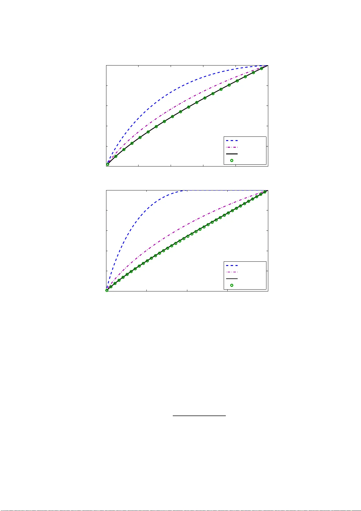
Sp ectrum Estimatio n: A Uniﬁed F ramew ork for Co v ariance Matrix Estimation and PCA in Large Dimensions ∗ Olivier Ledoit Departmen t o f E conomics Univ ersit y of Zuric h CH-8032 Zuric h, Switzerland olivier.ledoit@econ.uzh.c h Mic hael W olf † Departmen t of Economics Univ ersit y of Zurich CH-8032 Zuric h, Switzerland mic hael.w olf@econ.uzh.c h First v ersion: Janu ary 201 3 This v ersion: July 2013 Abstract Cov ar iance matrix estimation a nd principal component analys is (PCA) are tw o cor- nerstones of multiv ar iate ana lysis. Classic textbo ok solutions p erform po orly when the dimension of the data is of a magnitude similar to the sample size, or ev en larger. In such settings, there is a common remedy for bo th statistical problems: nonline ar shrink- age of the eigenv alues of the sample cov aria nce matrix. The o ptimal nonlinea r shrink ag e formula depends on unkno wn populatio n quan tities and is th us no t av a ila ble. It is, ho w- ever, po ssible to co ns isten tly e s timate an ora cle nonlinear shrink age, which is motiv ated on asymptotic grounds. A key to o l to this end is c o nsisten t estimatio n o f the set of eigenv al- ues of the populatio n cov aria nce matrix (als o kno wn as the sp e ctru m ), an interesting and challenging problem in its own right. E xtensiv e Monte Carlo simulations demonstrate that our methods hav e de s irable ﬁnite-sample prop erties and outperfor m previous propo sals. KEY W ORDS: Large-dimensional asymp tot ics, co v ariance matrix eigenv alues, nonlinear shr ink age, p rincipal comp onen t analysis. JEL CLAS SIFICA TION NO S: C13. ∗ Researc h was partially completed while b oth auth ors w ere visiting the Institute for Mathematical Sciences, National Universit y of Singapore in 2012. † Researc h has b een supp orted by the NCCR Finrisk pro ject “New Metho d s in Theoretical and Empirical Asset Pricing”. 1 1 In tro du c tio n This paper tac kles thr ee imp ortan t problems in multiv ariate statistics: 1) the estimation of the eigen v alues of the co v ariance matrix; 2 ) the estimation of the cov ariance matrix itself; and 3) principal comp onent analysis (PC A). In many mo dern app lications, the matrix di- mension is not negligible w ith resp ect to the sample size, so textb o ok solutions b ased on classic (ﬁxed-dimension) asymptotics are no longer appr opriate. A b etter-suited framewo rk is lar ge- dimensiona l asymptotics , where the matrix dimension and the sample size go to inﬁ nit y together, w hile their ratio — called the c onc entr ation — con verge s to a ﬁnite, nonzero limit. Under large-dimensional asymp to tics, the samp le co v ariance matrix is no longer consisten t, and neither are its eigenv alues nor its eigen ve ctors. One of the inte resting f eatures of large-dimensional asymptotics is that principal comp o- nen t analysis can no longer b e conducted u s ing co v ariance matrix eigen v alues. Th e v ariation explained b y a principal comp onent is not equal to the corresp ondin g sample eigen v alue and — p erhaps more sur prisingly — it is not equal to the corresp ondin g p opu lat ion eigen v alue either. T o the b est of our kno w ledge, this fact has not b een noticed b efore. The v ariation exp lai ned b y a p rincipal comp onent is obtained ins tead b y applying a nonline ar shrinkage formula to the corresp onding sample eigenv alue. This nonlinear shrink age formula dep ends on the u nobserv- able p opulation cov ariance matrix, but th an k f ully it can approximate d by an or acle shrinkage form ula w hic h d epend s ‘o nly’ on the un observ able eigen v alues of the p opulation co v ariance matrix. This is the connectio n with the ﬁrs t of the three p roblems mentioned ab o ve . Once w e ha v e a consisten t estimator of the p opulation eigen v alues, we can use it to deriv e a consisten t estimator of the oracle sh rink age. The connection with the second pr oblem, the estimation of the whole co v ariance matrix, is that the n onlinear shrink age formula that giv es the v ariation exp lai ned b y a p rincipal comp o- nen t also yields the optimal rotation-equiv ariant estimato r of the co v ariance matrix acc ording to the F rob en ius norm. Thus, if we can consistent ly estimate the p opulation eig env alues, and if we plug them in to the oracle shr ink age formula, we can addr ess the problems of PCA and co v ariance matrix estimation in a uniﬁed framewo rk. It needs to p oin ted out there that in a r ota tion-equiv arian t framew ork, consisten t (or ev en impro v ed) estimators of the p opulation eigen v alues are not av ailable; ins te ad, one needs to retain the sample eigen ve ctors. As a consequence, consistent estimation of the p opu la tion co- v ariance matrix itself is n ot p ossible. Nev ertheless, a r ota tion-equiv arian t estimator can still b e v ery useful for p r act ical applications, as evidenced by the p opu larit y of the pr evious prop osal of Ledoit and W ol f (20 04). An alternativ e approac h that wo uld allo w for consisten t estimat ion of the p opulatio n co v ariance matrix is to imp ose additional str u cture on the estimation prob- lem, suc h as s parseness, a graph mo del, or an (appro ximate) factor mo del. But wh ether suc h structure do es ind ee d exist is something that cannot b e v eriﬁed from the data. Th erefore, at least in some applications, a structure-free approac h will b e preferred by applied researc hers. This is the problem that we addr ess, aiming to f u rther imp ro ve u p on Ledoit and W olf (2004). Of course estimating p opulation eigen v alues co nsistently u n der large-dimensional asymp- 2 totics is no trivial matter. Un til recen tly , most researc hers in t he ﬁeld eve n feared it might b e imp ossible b ecause deducing p opulation eigenv alues from sample eigen v alues sho wed some symptoms of il l-p ose dness . This means that small estimation errors in the sample eigen v al- ues w ould b e ampliﬁed b y the sp eciﬁc mathematical structur e of the asymp to tic r elationship b et ween sample and p opulation eigen v alues. But t wo recen t articles by Mestre (2008) and El Karoui (200 8 ) chal lenged this widely-held b elief and ga ve some hop e that it migh t b e p os- sible after all to estimate th e p opu lati on eigen v alues consistent ly . Still, a general satisfact ory solution is not a v ailable to date. The work of Mestre (2008) only app lies when the num b er of distinct p opu lat ion eigenv alues remains ﬁnite as matrix dimens io n go es to inﬁnit y . In practice, this means that th e num b er of distinct eigen v alues must b e negligible with resp ect to the total num b er of eigen v alues. As a further restriction, the n umber of distinct eigen v alues and their multiplici ties m ust b e kno wn. The only un kno wn quantitie s to b e estimated are the lo catio ns of the eigenv alues; of cours e, this is still a diﬃcult task. Y ao et al. (2012) prop ose a more general estimation pro cedure that do es not require kno wledge of the multipliciti es, though it still requires knowle dge of the n umb er of d istinct p opulation eigen v alues. This setting is too restrictiv e for man y applications. The metho d dev elop ed by El Karoui (20 08) allo ws for an arbitrary set of p opulation eigen- v alues, but does not app ear to ha v e go od ﬁ n ite- sample prop erties. In fact, our simulatio ns seem to indicate that this estimator is not ev en consisten t; see Section 5.1.1. The ﬁrst contribution of the p resen t p ap er is, therefore, to dev elop an estimato r of th e p opulation eigen v alues t hat is consistent under large-dimensional asymptotics r e gar d less of whether or n ot they are clustered, and that also p erforms w ell in ﬁ n ite sample. T his is ac h iev ed through a more precise c haracterization of the asymp totic b ehavio r of sample eigen v alues. Whereas existing results only sp ecify ho w the eigen v alues b eha v e on a v erage, namely , how man y fall in any giv en int erv al, w e determine individual limits. Our second con tribu tio n is to s ho w how this consistent estimator of p opulation eigen v alues can b e u sed for imp ro ve d estimation of the co v ariance matrix when the d imension is large compared to the samp le size. This w as already considered in Ledoit and W ol f (2012), but only in the limited setup where the dimension is smaller than the sample size. Thanks to the adv ances introdu ced in the pr esen t p aper, w e can also handle the more diﬃcult case where the dimension exceeds the sample size and the sample co v ariance matrix is singular. Our th ir d and ﬁnal contribution is to sh o w how the same nonlinear shrink age f orm ula can b e used to estimate the fraction of v ariation explained by a giv en collection of p r incipal comp onen ts in PCA, whic h is k ey in deciding h ow many principal comp onen ts to retain. The remaind er of the pap er is organized as follo ws. Section 2 p resen ts our estimator of the eige nv alues of the popu lati on co v ariance matrix und er large-dimensional asymptotics. Section 3 discusses co v ariance matrix estimati on, and Section 4 principal comp onen t analysis. Section 5 stud ies ﬁnite-sample p erformance via Mont e C arlo sim u lati ons. Sect ion 6 provides a br ief empirical application of PCA to stock return data. Section 7 concludes. The pro ofs of all mathematical results are collected in the app endix. 3 2 Estimation of P opulation Co v ariance Matrix Eigen v alues 2.1 Large-Dimensiona l Asymptotics and Basic F ramew ork Let n denote the sample size an d p . . = p ( n ) the n umb er of v ariables. It is assumed that the ratio p/n conv erges as n → ∞ to a limit c ∈ (0 , 1) ∪ (1 , ∞ ) called the c onc entr ation . T he case c = 1 is ru led ou t for tec hnical reasons. W e mak e the follo wing assump tions. (A1) T h e p opu lat ion co v ariance matrix Σ n is a n on r andom p -d im en sional p ositiv e d eﬁnite matrix. (A2) X n is an n × p matrix of real indep end en t and id en tically distributed (i.i.d.) random v ariables with zero mean, unit v ariance, and ﬁn ite fourth momen t. On e only obs erv es Y n . . = X n Σ 1 / 2 n , so n either X n nor Σ n are observ ed on their o wn. (A3) τ n . . = ( τ n, 1 , . . . , τ n,p ) ′ denotes a system of eigen v alues of Σ n , sorted in increasing order, and ( v n, 1 , . . . , v n,p ) denotes an associated system of eigen v ectors. Th e empirical distri- bution function (e.d.f.) of the p opulation eigen v alues is d eﬁ ned as: ∀ t ∈ R , H n ( t ) . . = p − 1 P p i =1 1 [ τ n,i , + ∞ ) ( t ), where 1 denotes the indicator function of a set. H n is called the sp e ctr al distribution (function) . It is assumed that H n con verges weakly to a limit law H , called the limiting sp e c tr al distribution (function) . (A4) S upp ( H ), the supp ort of H , is the un io n of a ﬁnite num b er of close d inte rv als, b ounded a wa y from zero and inﬁnity . F urthermore, there exists a compact in terv al in (0 , ∞ ) that con tains Supp ( H n ) for all n large enough. Let λ n . . = ( λ n, 1 , . . . , λ n,p ) ′ denote a sys te m of eigen v alues of the sample co v ariance m a- trix S n . . = n − 1 Y ′ n Y n = n − 1 Σ 1 / 2 n X ′ n X n Σ 1 / 2 n , sorted in increasing o rder, and let ( u n, 1 , . . . , u n,p ) denote an asso ciate d s y s te m of eigen v ectors. The ﬁrst sub script, n , ma y b e omitted when no confus ion is p ossible. Th e e.d.f. of the sample eigen v alues is deﬁned as: ∀ t ∈ R , F n ( t ) . . = p − 1 P p i =1 1 [ λ i , + ∞ ) ( t ). The literature on the eigenv alues of samp le co v ariance matrices un der large-dimensional asymp tot ics — also kno wn as r andom matrix the ory (RMT) literature — is based on a f oundational result due to Mar ˇ cenk o and Pastur (1967). It h as b een strengthened and broadened by su b sequen t authors in cluding Silverstein (1995), Silverstei n and Bai (1995), Silv erstein and Choi (1995), and Bai and Silv erstein (1998, 1999), among others . T hese arti- cles imply that there exists a limiting sample sp ectral distribution F suc h th at ∀ x ∈ R \ { 0 } F n ( x ) a . s . − → F ( x ) . (2.1) In other words, the aver age n umb er of sample eigen v alues falling in an y giv en in terv al is kno wn asymptotically . In addition, the existing literature has unearthed imp ortant information ab out the limiting distribution F . Silv erstein and Choi (1995) show that F is everywhere contin uous except (p oten tially) at zero, and that the mass that F places at zero is given b y F (0) = max n 1 − 1 c , H (0) o . (2.2) 4 F ur thermore, there is a seminal equation relating F to H an d c . Some additional notation is required to presen t this equatio n. F or any n ondecreasing fun ctio n G on the real line, m G denotes the Stieltjes tr ansform of G : ∀ z ∈ C + m G ( z ) . . = Z 1 λ − z dG ( λ ) , where C + denotes the half-plane of complex n umb ers with strictly p ositiv e imaginary part. The Stieltjes transform admits a w ell-kno wn inv ersion form ula: G ( b ) − G ( a ) = lim η → 0 + 1 π Z b a Im  m G ( ξ + iη )  dξ , (2.3) if G is con tinuous at a and b . Here, and in the remainder of th e pap er, w e shall u s e the notatio ns Re ( z ) and Im ( z ) for the real and imaginary p arts, resp ectiv ely , of a co mplex num b er z , so that ∀ z ∈ C z = Re ( z ) + i · Im ( z ) . The most elegan t ve rsion of the equatio n relating F to H and c , due to Silve rstein (1995), states that m . . = m F ( z ) is th e unique solution in the set  m ∈ C : − 1 − c z + cm ∈ C +  (2.4) to the equation ∀ z ∈ C + m F ( z ) = Z 1 τ  1 − c − c z m F ( z )  − z dH ( τ ) . (2.5) As explained, the Stieltjes transform of F , m F , is a fun ctio n whose domain is the up p er half of the complex p lane. It can b e extended to the r eal line, since Silv erstein and Choi (1995) sho w that: ∀ λ ∈ R \ { 0 } , lim z ∈ C + → λ m F ( z ) = . . ˘ m F ( λ ) exists. When c < 1, ˘ m F (0) also exists and F has a contin uous deriv ativ e F ′ = π − 1 Im [ ˘ m F ] on all of R with F ′ ≡ 0 on ( −∞ , 0]. (On e should rememb er that although the argument of ˘ m F is real-v alued no w, the ou tp ut of the function is still a complex n umb er.) F or p urp oses that will b eco me apparent later, it is useful to reform ulate equation (2.5). The limiting e.d.f. of the eigen v alues of n − 1 Y ′ n Y n = n − 1 Σ 1 / 2 n X ′ n X n Σ 1 / 2 n w as d eﬁned as F . In addition, deﬁne the limiting e.d.f. of the eigen v alues of n − 1 Y n Y ′ n = n − 1 X n Σ n X ′ n as F ; note that the eigen v alues of n − 1 Y ′ n Y n and n − 1 Y n Y ′ n only diﬀer b y | n − p | zero eigen v alues. It then holds: ∀ x ∈ R F ( x ) = (1 − c ) 1 [0 , ∞ ) ( x ) + c F ( x ) (2.6) ∀ x ∈ R F ( x ) = c − 1 c 1 [0 , ∞ ) ( x ) + 1 c F ( x ) (2.7) ∀ z ∈ C + m F ( z ) = c − 1 z + c m F ( z ) (2.8) ∀ z ∈ C + m F ( z ) = 1 − c c z + 1 c m F ( z ) . (2.9) 5 (Recall here that F has mass ( c − 1) /c at zero when c > 1, so that b oth F and F are n onnegat ive functions ind eed for an y v alue c > 0.) With this notation, equatio n (1.13) of Mar ˇ cenk o and P astur (1967) reframes equation (2.5 ) as: f or eac h z ∈ C + , m . . = m F ( z ) is the un ique s ol ution in C + to the equation m = −  z − c Z τ 1 + τ m dH ( τ )  − 1 . (2.10) While in the case c < 1, ˘ m F (0) exists and F is cont inuously diﬀeren tiable on all of R , as men tioned ab o ve, in the case c > 1, ˘ m F (0) exists and F is con tinuously diﬀerentiable on all of R . 2.2 Individual Beha vior of Sampl e Eigenv alues: the QuEST F unction W e introdu ce a nonr andom m ultiv ariate function called the Quantize d Eigenvalues Sampling T r ansform , or Q uEST for short, whic h d iscretiz es, or quantizes , the relationship b et ween F , H , and c deﬁned in equations (2.1)–(2.3). F or an y p ositiv e in tegers n and p , the Q u EST f unction, denoted by Q n,p , is deﬁned as Q n,p : [0 , ∞ ) p − → [0 , ∞ ) p (2.11) t . . = ( t 1 , . . . , t p ) ′ 7− → Q n,p ( t ) . . =  q 1 n,p ( t ) , . . . , q p n,p ( t )  ′ , (2.12) where ∀ z ∈ C + m . . = m t n,p ( z ) is the unique solution in the s et  m ∈ C : − n − p nz + p n m ∈ C +  (2.13) to the equation m = 1 p p X i =1 1 t i  1 − p n − p n z m  − z , (2.14) ∀ x ∈ R F t n,p ( x ) . . =          max ( 1 − n p , 1 p p X i =1 1 { t i =0 } ) if x = 0 , lim η → 0 + 1 π Z x −∞ Im  m t n,p ( ξ + iη )  dξ otherwise , (2.15) ∀ u ∈ [0 , 1]  F t n,p  − 1 ( u ) . . = sup { x ∈ R : F t n,p ( x ) ≤ u } , (2.16) and ∀ i = 1 , . . . , p q i n,p ( t ) . . = p Z i/p ( i − 1) /p  F t n,p  − 1 ( u ) du . (2.17) It is obvious that equation (2.13) qu an tizes equation (2.4), that equation (2.14) quanti zes equation (2.5), and that equation (2.15) quan tizes equations (2.2) and (2.3). Thus, F t n,p is the limiting d istr ibution (fun ction) of sample eigen v alues corresp onding to the p opulation sp ectral distribution (function) p − 1 P p i =1 1 [ t i , + ∞ ) . F ur thermore, b y equation (2.16),  F t n,p  − 1 represent s the inv erse sp ectral distribution fu n ctio n, also kno wn as the quantile function. 6 Remark 2.1 (Deﬁnition of Quan tiles) . The stand ard deﬁnition of the ( i − 0 . 5) / p quantil e of F t n,p is  F t n,p  − 1 (( i − 0 . 5) /p ), wh er e  F t n,p  − 1 is deﬁned in equatio n (2.16). It turns o ut, ho w ev er, that the ‘smo othed’ v ersion q i n,p ( t ) giv en in equation (2.17) leads to impro v ed ac- curacy , higher stabilit y , and faster computatio ns of our numerical algorithm, to b e deta iled b elo w, in practice. Since F n is an empirical distribution (fun ctio n), its quantil es are not un iquely d eﬁned. F or example, the statistical soft w are R oﬀers nine diﬀeren t v ersions of samp le quan tiles in its function quantile ; v ersion 5 corresp onds to our con ven tion of considering λ n,i as the ( i − 0 . 5) /p quan tile of F n . Consequent ly , a set of ( i − 0 . 5) / p quantile s ( i = 1 , . . . , p ) is giv en by Q n,p ( t ) for F t n,p and is giv en by λ n for F n . The r ela tionship b etw een Q n,p ( t ) and λ n is fu rther elucidated by the follo wing theorem. Theorem 2.1. If Assumptions (A1)–(A4) ar e satisﬁe d, then 1 p p X i =1  q i n,p ( τ n ) − λ n,i  2 a . s . − → 0 . (2.18) Theorem 2.1 states that the sample eigen v alues conv erge individu all y to their nonr andom QuEST function count erparts. This individual notion of conv ergence is d eﬁ ned as the Euclidian distance b et ween the v ectors λ n and Q n,p ( τ n ), normalized by the matrix dimension p . It is the appropriate normalization b ecause, as p go es to inﬁnit y , the left-hand sid e of equation (2.18 ) appro ximates the L 2 distance b etw een the functions F − 1 n and  F τ n n,p  − 1 . This metric ca n b e though t of as a ‘cross-sectional’ mean squared error, in th e same w a y that F n is a cross-sectional distribution f unction. Theorem 2.1 imp r o v es o ver th e well-kno wn results from the random matrix theory literature review ed in Section 2.1 in t w o signiﬁcan t w a ys. 1) It is based on the p p opu lation eigenv alues τ n , not the limiting sp ectral distrib ution H . Dealing with τ n (or, equiv alen tly , H n ) is straight forward b ecause it is in tegral to the actual data-generating p rocess; wh ereas d eal ing with H is more delicate b ecause w e do not know how H n con verges to H . Also there are p oten tially d iﬀeren t H ’s that H n could con verge to, dep ending on what w e assume will happ en as the dimension increases. 2) Th eorem 2.1 c haracterizes th e individual b eha vior of the samp le eigen v alues, whereas equation (2.1) only c haracterizes their aver age b ehavio r, namely , wh at prop ortion f all s in an y giv en inte rv al. Ind ividual results are more precise th an a v erage results. Thus, The- orem 2.1 sho ws that the sample eigen v alues are b etter b ehav ed under large-dimensional asymptotics th an previously thought. Both of these improv emen ts are mad e p ossible th anks to the int ro duction of the QuES T function. In spite of the apparen t c omplexit y of the mathematical deﬁnition of the QuEST function, it can b e compu ted quickly and eﬃcien tly along with its analytical Jacobian as evidenced by Figure 1, and it b eha ve s w ell numericall y . 7 0 200 400 600 800 1000 0 0.5 1 1.5 Matrix Dimension p Seconds Average Computation Time QuEST Function Analytical Jacobian Figure 1: Averag e computation time for the Qu EST f u nction and its analytica l Jacobian. The setup is the same as in Fig ure 2 b elo w. The QuEST function and its analytica l Jacobian are programmed in Matla b. T h e computer is a 2 . 4 GHz d esktop Mac. 2.3 Consisten t Est ima tion of P opulation Eigen v alues Once the truth of Th eorem 2.1 h as b een established, it b ecomes tempting to construct an estimator of p opulation co v ariance matrix eige nv alues simply b y minimizing th e expression on the left-hand side of equation (2.18) ov er all p ossible sets of p opulation eigen vec tors. Th is is exactly wh at we do in the follo wing theorem. Theorem 2.2. Supp ose that Assumptions (A1)–(A4) ar e satisﬁe d. Deﬁne b τ n . . = argmin t ∈ [0 , ∞ ) p 1 p p X i =1  q i n,p ( t ) − λ n,i  2 , (2.19) wher e λ n . . = ( λ n, 1 , . . . , λ n,p ) ′ ar e the sample c ovarianc e matrix e i genvalues, and Q n,p ( t ) . . =  q 1 n,p ( t ) , . . . , q p n,p ( t )  ′ is the nonr andom Q uEST function deﬁne d in e quations (2.11) – (2.1 4 ) ; b oth b τ n and λ n ar e assume d sorte d in incr e asing or der. L et b τ n,i denote the i th entry of b τ n ( i = 1 , . . . , p ) , and let τ n . . = ( τ n, 1 , . . . , τ n,p ) ′ denote the p opulation c ovarianc e matrix eigenvalues sorte d in incr e asing or der. Then 1 p p X i =1 [ b τ n,i − τ n,i ] 2 a . s . − → 0 . (2.20) Theorem 2.2 shows that the estimated eigen v alues con ve rge individual ly to the p opulation eigen v alues, in the same sens e as ab o ve, usin g the dimension-normalized Eu clidian distance. Remark 2.2. Mathemati cally sp eaking, equation (2.19) perf orms tw o tasks: it p ro jects λ n on to the image of the QuEST function, and then in verts the QuES T function. Since the imag e of the QuEST function is a str ict s u bset of [0 , ∞ ) p , λ n will generally b e ou tsid e of it. It is the ﬁrst of these t wo tasks that gets around any p ote nti al ill-p osedness b y r e gularizing the set of observ ed samp le eigen v alues. 8 Practically sp eaking, b oth tasks are p erf orm ed simultaneo usly b y a nonlinear optimizer. W e use a standard oﬀ-t he-shelf commercial softw are called SNOPT TM (V ersion 7.4), see Gill et al. (2002), bu t other c h oices ma y w ork w ell to o. 2.4 Comparison with Other Approach es El Karoui (2008) also attempts to discretize equation (2.5) and in v ert it, bu t h e opts for a completely opp osite metho d of discretization whic h do es not exploit the natural d iscr eteness of the p opu lat ion sp ectral distribu tion for ﬁnite p . If the p opulation sp ectral distribution H n is approximat ed b y a con ve x linear combination of step functions ∀ x ∈ R e H ( x ) . . = p X i =1 w i 1 { x ≥ t i } where ∀ i = 1 , . . . , p t i ≥ 0 , w i ≥ 0 , and p X i =1 w i = 1 , then in th e optimization problem (2.19), we kee p the weig hts w i ( i = 1 , . . . , p ) ﬁxed at 1 /p wh ile v arying the lo cation parameters t i ( i = 1 , . . . , p ). In con trast, El Karoui (2008) d oes exactly the rev erse: he k eeps the lo catio n parameters t i ﬁxed on a grid while v arying the w eigh ts w i . Th us, El Karoui (2008) pro jects the p opulation sp ectral distribution on to a “dictionary”. F ur - thermore, instead of matc hing p opulation eigenv alues to sample eigen v alues on R , he matc hes a f unction of m e H to a function of m F n on C + , which make s his a lgorithm r ela tiv ely co mpli- cated; see Ledoit and W olf (2012, p ag es 1043– 1044). Despite our b est eﬀorts, w e w ere unable to replicate his co nv ergence results in Monte Carlo sim ulations: in our implementa tion, his estimator p erforms p o orly o verall and d oes not ev en app ear to b e consistent; see Section 5.1.1. Unless someone circulates an implemen tation of the algorithm d escrib ed in El K aroui (20 08 ) that works, w e hav e to write oﬀ this app roac h as impractical. Another related pap er is the one b y Ledoit and W olf (2012). They use the same discretiza- tion strategy as El K aroui (2008) (ﬁx lo cation parameters and v ary we igh ts) but, as we do here, matc h p opulation eigen v alues to sample eigen v alues on the real line. Unlik e w e do here, they measure closeness b y a sup-distance rather th an b y the Eu clidea n d istance . Ledoit an d W olf (2012) only consider the case p < n . Unfortun ate ly , their nonlinear optimizer no longer con- v erges reliably in the case p > n , as we found out in sub sequen t exp erimen ts; this necessitated the d ev elopment of the alternativ e discretization strategy d escrib ed ab o ve, as we ll as the c hange from sup -distance to Euclidean d istance to measure closeness. F ur thermore, Ledoit and W olf (2012) are not directly interested in estimating the p opu- lation eige nv alues; it is just an in termediary step to wards their u ltimat e ob jectiv e, which is the estimatio n of the co v ariance m at rix itself. Therefore they d o not rep ort an y Monte Carlo sim ulations on the ﬁn ite-sample b eha vior of their estimator of the p opulation eigenv alues. In any case, the aim of the pr esent pap er is to develo p an estimator of the p opulation eigen v alues that wo rks also when p > n , so the approac h of Ledoit and W olf (201 2 ) is ruled out. The d iﬀeren t discretization str at egy that w e emplo y here, together with the alternativ e distance measure, enables us to construct an estimator of τ n that wo rks across b oth cases p < n and p > n . It is imp ortant to p oin t out that the new estimator of p opulation eigen v alues 9 is not only more general, in the sense th at it also works for the case p > n , but it also w orks b etter for the case p < n ; see S ecti on 5.2. As for the pap ers of Mestre (2008) and Y ao et al. (2012), their metho ds are based on con tour int egration of analytic functions in the complex plane. They can only extract a ﬁ n ite n umb er ¯ M of functionals of H n , such as the lo cati ons of high-m u ltiplici t y eigen v alue clusters, or the trace of p ow ers of Σ n . The main diﬀerence with our metho d is that w e extract man y more items of information: namely , p p opulation eigenv alues. This distinction is crucial b ecause th e ratio ¯ M /p v anishes asymptotically . It explains why we are able to reco ver the whole p opulation sp ectrum in the general case, w hereas they are not. 3 Co v ariance Matrix Estimation The estimat ion of the co v ariance matrix Σ n is already considered b y Ledoit and W olf (2012), but only for the case p < n . In particular, they prop ose a nonlinear shrink age approac h, whic h w e will no w extend to the case p > n . T o sa ve space, the reader is referred to their pap er for a more detailed d iscussion of the nonlinear shrink age metho d olo gy and a comparison to other estimation strategies of large-dimensional co v ariance matrices, su c h as the linear sh rink age estimator of Ledoit and W olf (2004). 3.1 Oracle Shrink age The starting p oint is to restrict atten tion to r otation-e quivariant estimators of Σ n . T o b e more sp eciﬁc, let W b e an arbitrary p -dimensional rotation m atrix. Let b Σ n . . = b Σ n ( Y n ) b e an estimator of Σ n . Then the estimator is said to b e r otation-e quivariant if it satisﬁes b Σ n ( Y n W ) = W ′ b Σ n ( Y n ) W . In other wo rd s , the estimate based on th e r ot ated data equals the r otation of the estimate based on the original data. In the absence of an y a pr iori kno wledge ab out the structure of Σ n , suc h as sp arseness or a facto r mo del, it is natural to consider only estimators of Σ n that are rotatio n-equiv ariant. The class of rotatio n-equiv ariant estimators of the co v ariance that are a function of the sample co v ariance m atrix is constituted of all the estimators that ha v e the same eigen ve ctors as the sample co v ariance matrix; for exa mple, see P erlman (2007, Section 5.4). Ev ery suc h rotation-equiv ariant estimator is thus of the form U n D n U ′ n where D n . . = Diag ( d 1 , . . . , d p ) is diago nal , (3.1) and where U n is the matrix whose i th column is the sample eigenv ector u i . . = u n,i . This is the class of rotatio n-equiv ariant estimators already stu died b y Stein (1975, 1986). W e can rewrite the expression for suc h a rotation-equiv ariant estimator as U n D n U ′ n = p X i =1 d i · u i u ′ i . (3.2) This alternativ e expression sho ws that any suc h rotation-equiv ariant estimator is a linear com- bination of p r ank-1 matrices u i u ′ i ( i = 1 , . . . , p ). But since the { u i } form an orthon orm al basis 10 in R p , the resulting estimator is still of full rank p , provided that all the w eigh ts d i ( i = 1 , . . . , p ) are strictly p ositiv e. Remark 3.1 (Rotation-equiv arian t Estimat ors versus Structur ed Estimators) . By construc- tion, the class (3.1) of rotation-in v arian t estimators ha ve the same eigen v ectors as the sample co v ariance matrix. In particular, consisten t estimatio n of the co v ariance matrix is not p ossible under large-dimensional asymptotics. Another approac h w ould b e to imp ose add itional structure on the estimation problem, suc h as spars eness (Bic ke l and Levina, 2008), a graph mo del (Ra jaratnam et al., 2008), or an (appr o ximate) factor mo del (F an et al., 2008). 1 The adv an tage of doing so is that, und er suitable regularit y conditions, consistent estimation of the co v ariance matrix is p ossib le. The disadv ant age is that if the assumed s tructure is missp eciﬁed, the estimator of the cov ariance matrix c an be arbitrarily bad; and w hether the stru cture is correctly sp eciﬁed ca n nev er b e v eriﬁed fr om the data alone. Rotation-e quiv ariant estimators are widely and su ccessfu lly used in p racti ce in situations where knowledge on ad d itio nal structur e is not a v ailable (or doubtfu l). This is evidenced b y the man y citations to Ledoit and W olf (2004) w ho prop ose a lin ear shrink age estimator that also b elongs to the class (3.1); for example, s ee the b eginnin g of Section 5.2. Therefore, dev eloping a new, nonlinear shrink age estimator that outp erforms this previous prop osal will b e of subs ta ntia l in terest to app lied researc hers in our opinion. The ﬁ rst ob jectiv e is to ﬁnd the matrix in the class (3.1) of rotatio n-equiv ariant estimat ors that is closest to Σ n . T o measure distance, we c ho ose the F rob enius n orm deﬁned as || A || F . . = p T r ( AA ′ ) /r for any matrix A of dimension r × m . (3.3) (Dividing b y the dimension of the square matrix AA ′ inside the ro ot is n ot standard, but w e do this for asymptotic purp oses so that the F rob enius n orm remains constant equal to one for the iden tit y matrix regardless of the dimension; see Ledoit and W olf (2004).) As a result, w e end up with the follo wing minimization p roblem: min D n || U n D n U ′ n − Σ n || F . Elemen tary m atrix algebra sh o ws th at its solution is D ∗ n . . = Diag ( d ∗ 1 , . . . , d ∗ p ) where d ∗ i . . = u ′ i Σ n u i for i = 1 , . . . , p . (3.4) Let y ∈ R p b e a random ve ctor with co v ariance matrix Σ n , dr a wn indep endentl y from the sample co v ariance matrix S n . W e can think of y as an out-of-sample observ ation. T hen d ∗ i is recognized as the v ariance of the lin ea r combinatio n u ′ i y , cond itio nal on S n . In v iew of the expression (3.2), it mak es in tuitiv e sense that the matrices u i u ′ i whose associated linear com b inatio n u ′ i y ha v e h igher out-o f-sample v ariance sh ould receiv e higher w eigh t in computing the estimator of Σ n . 1 W e only give one rep resen tative reference fo r each ﬁ eld here to sav e space. 11 The ﬁn ite -sample optimal estimator is th u s giv en by S ∗ n . . = U n D ∗ n U ′ n where D ∗ n is deﬁned as in (3.4) . (3.5) Clearly S ∗ n is not a fe asible estimato r b ecause it dep ends on knowing the p opulation co v ari- ance matrix. By generali zing th e Mar ˇ cenk o-P astur equation (2.5), Led oi t and P ´ ec h´ e (2011) sho w that d ∗ i can b e app ro ximated b y the asymptotic qu an tities d or i . . =          1 ( c − 1) ˘ m F (0) , if λ i = 0 and c > 1 λ i   1 − c − c λ i ˘ m F ( λ i )   2 , otherwise for i = 1 , . . . , p , (3.6) from wh ic h they deduce their oracl e estimator S or n . . = U n D or n U ′ n where D or n . . = Diag ( d or 1 , . . . , d or p ) . (3.7) The key d iﬀerence b et wee n D ∗ n and D or n is that th e form er dep ends on the unobserv able p opulation co v ariance matrix, wh ereas the latter dep ends on the limiting distrib ution of sample eigen v alues, F , which mak es it amenable to consisten t estimation. It turns out that this estimation problem is solv ed if a consisten t estimator of the p opulation eigen v alues τ n is a v ailable. 3.2 Nonlinear Shrink age Estimator 3.2.1 The Case p < n W e start with the case p < n , wh ich w as already considered by L ed oit and W olf (2012). Silv erstein and Choi (1995) show ho w th e sup p ort of F , denoted by Supp ( F ), is determined; also see Section 2.3 of Ledoit and W olf (2012 ). S upp ( F ) is seen to b e the union of a ﬁnite n umb er of disjoin t compact in terv als, b ounded aw a y from zero. T o simplify the discussion, we will assum e fr om here on that Supp ( F ) is a single compact in terv al, b ounded a w a y from zero, with F ′ > 0 in the in terior of this int erv al. But if Supp ( F ) is the u nion of a ﬁnite num b er of suc h in terv als, the argum en ts presen ted in this sectio n as wel l as in th e remainder of the pap er apply separately to eac h in terv al. In p artic ular, our consistency results p resen ted b elo w can b e easily extended to this m ore general case. Recall that, f or an y t . . = ( t 1 , . . . , t p ) ′ ∈ [0 , + ∞ ) p , equations (2.13)–(2.14) deﬁne m t n,p as th e Stieltjes transform of F t n,p , the limiting distribu tio n of samp le eigen v alues corresp ondin g to the p opulation sp ectral distribution p − 1 P p i =1 1 [ t i , + ∞ ) . Its domain is the strict upp er half of the complex plane, b ut it can b e exte nd ed to the real line since Silverstein and C hoi (199 5 ) pro ve that ∀ λ ∈ R − { 0 } lim z ∈ C + → λ m t n,p ( z ) = . . ˘ m t n,p ( λ ) exists. Ledoit and W olf (2012) sh ow ho w a consistent estimator of ˘ m F can b e derived from a consisten t estimator of τ n , such as b τ n deﬁned in Theorem 2.2 . Their Prop osition 4.3 establishes that ˘ m b τ n n,p ( λ ) → ˘ m F ( λ ) u n iformly in λ ∈ Supp ( F ), except for t wo arbitrarily small regions at the 12 lo wer and upp er end of S upp ( F ). Replacing ˘ m F with ˘ m b τ n n,p and c with p/n in Ledoit and P ´ ech ´ e (2011)’s oracle quan tities d or i of (3.6) yields b d i . . = λ i    1 − p n − p n λ i · ˘ m b τ n n,p ( λ i )    2 for i = 1 , . . . , p . (3.8) (Note here that in the case p < n , all sample eigen v alues λ i are p ositiv e almost su rely , for n large e nough, by the results of Bai and Silve rstein (1998).) In turn, the b ona ﬁde nonlinear shrink age estimator of Σ n is obtained as: b S n . . = U n b D n U ′ n where b D n . . = Diag ( b d 1 , . . . , b d p ) . (3.9) 3.2.2 The Case p > n W e mo v e on to the case p > n , whic h wa s not considered by L edoit and W olf (2012). In this case, F is a mixture distribution with a discrete part and a con tin uous part. Th e discrete part is a p oin t mass at zero w ith mass ( c − 1) /c . Th e con tinuous part h as total mass 1 /c and its supp ort is the union of a ﬁnite num b er of d isjoin t in terv als, b ound ed aw a y f rom zero; again, see Silverstei n and Ch oi (19 95). It can b e seen fr om equations (2.6)–(2.9) that F corresp onds to the con tinuous part of F , scaled to b e a prop er distribu tio n (fu nction): lim t →∞ F ( t ) = 1. Consequen tly , Supp ( F ) = { 0 } ∪ Supp ( F ). T o simplify the discussion, w e w ill assume f rom here on th at S upp ( F ) is a single compact in terv al, b ounded a wa y f r om zero, w ith F ′ > 0 in the interior of this in terv al. But if S upp ( F ) is the union of a ﬁn ite num b er of su c h in terv als, the arguments presented in this section as w ell as in the remainder of the pap er apply separately to eac h interv al. In particular, our consistency results presen ted b elo w can b e easily extended to th is more general case. The oracle qu an tities d or i of (3.6) in vo lv e ˘ m F (0) and ˘ m F ( λ i ) for v arious λ i > 0; r eca ll that ˘ m F (0) exists in the case c > 1. Using the original Mar ˇ cenko-P astur equation (2.10), a strongly consisten t estimato r of the quan tit y ˘ m F (0) is the uniqu e solution m . . = \ ˘ m F (0) in (0 , ∞ ) to the equation m = " 1 n p X i =1 b τ i 1 + b τ i m # − 1 , (3.1 0) where b τ n . . = ( b τ 1 , . . . , b τ p ) ′ is d eﬁned as in Theorem 2.2 . Again, since b τ n is consisten t for τ n , Prop osition 4.3 of Ledoit and W olf (2012) implies that ˘ m b τ n n,p ( λ ) → ˘ m F ( λ ) uniform ly in λ ∈ Supp ( F ), except for tw o a rbitrarily small r egi ons at the lo wer and upp er end of S upp ( F ). Finally , the b ona ﬁde nonlinear shrink age estimator of Σ n is obtained as (3.9) but no w with b d i . . =            λ i    1 − p n − p n λ i · ˘ m b τ n n,p ( λ i )    2 , if λ i > 0 1  p n − 1  \ ˘ m F (0) , if λ i = 0 for i = 1 , . . . , p , (3.11) 13 3.3 Strong Consistency The follo wing theorem establishes th at our n onlinear shrink age estimator, based on the estima- tor b τ n of Th eorem 2.2, is strongly consisten t for the oracle estimat or across b oth cases p < n and p > n . Theorem 3.1. L et b τ n b e an estimato r of the eigenvalues of the p opulation c ovarianc e matrix satisfying p − 1 P p i =1 [ b τ n,i − τ n,i ] 2 a . s . − → 0 . Deﬁne the nonline ar shrinkage estimator b S n as in (3.9) , wher e the b d i ar e as in (3.8) in the c ase p < n and as in (3.11) in the c ase p > n . Then || b S n − S or n || F a . s . − → 0 . Remark 3.2. W e ha v e to rule out the case c = 1 (or p = n ) for mathematical r ea sons. First, w e need S upp ( F ) to b e b ounded a wa y from zero to establish v arious consistency results. But wh en c = 1, then Supp ( F ) can start at zero, that is, there exists u > 0 su ch that F ′ ( λ ) > 0 for all λ ∈ (0 , u ). T his w as already established b y Mar ˇ cenk o and P astur (1967) for the sp ecial case when H is a p oin t mass at o ne. In particular, the resulting (standard) Mar ˇ cenk o-P astur distribu tion F has densit y function F ′ ( λ ) = ( 1 2 π λc p ( b − λ )( λ − a ) , if a ≤ λ ≤ b , 0 , otherwise , and has p oin t mass ( c − 1) /c at the origin if c > 1, w here a . . = (1 − √ c ) 2 and b . . = (1 + √ y ) 2 ; for example, see Bai and Silv erstein (2010, Section 3.3.1). Second, we also need the assump tion c 6 = 1 ‘directly’ in the pro of of Theorem 3.1 to demonstrate that the summand D 1 in (A.17) con verges to zero. Although the case c = 1 is not co v ered b y the mathematical treatmen t, w e can still add ress it in Mon te Carlo simulatio ns; see Section 5.2. 4 Principal Comp onen t Analysis Principal comp onen t analysis (PCA) is one of the oldest and b est-kno wn tec h niques of mul- tiv ariate analysis, dating bac k to P earson (1901) and Hotelling (1933); for a compr ehensiv e treatmen t, see J oll iﬀe (2002). 4.1 The Cen tral Idea and t he Common Practice The cen tr al idea of PCA is to reduce th e dimensionalit y of a data set consisting of a large n umb er of in terrelated v ariables, while r eta ining as muc h as p ossible of the v ariation p resen t in the data set. This is ac hieve d by transforming the original v ariables to a new set of unc orr elate d v ariables, the pr in cipal comp onen ts, wh ic h are ordered so that the ‘la rgest’ few retain most of the v ariation presen t in al l of the original v ariables. More sp eciﬁcally , let y ∈ R p b e a r andom v ector w ith co v ariance matrix Σ; in this section, it will b e conv enien t to dr op the subscript n f rom th e co v ariance m at rix and related quantiti es. Let (( τ 1 , . . . , τ p ); ( v 1 , . . . , v p )) d enote a system of eigen v alues and eigen ve ctors of Σ. T o b e 14 consisten t w ith our former notation, w e assume that the eig env alues τ i are sorted in incr e asing order. Then the principal comp onen ts of y are giv en by v ′ 1 y , . . . , v ′ p y . Since the eigen v alues τ i are sorted in increasing order, the pr incipal comp onen t with the largest v ariance is v ′ p y and the principal comp on ent with the smallest v ariance is v ′ 1 y . The eigen vect or v i is called the ve ctor of c o eﬃcients or lo adings for the i th pr incipal comp onen t ( i = 1 , . . . , p ). Tw o brief remarks are in ord er. First, some authors us e the term princip al c omp onents f or the eigen vect ors v i ; bu t we agree with Jolliﬀe (2002, Section 1.1) that this usage is confusing and that it is preferable to reserve the term for the deriv ed v ariables v ′ i y . Second, in th e PCA literature, in contrast to the bu lk of the multiv ariate statistics literature, th e eigen v alues τ i are generally sorted in decreasing order so that v ′ 1 y is the ‘largest’ pr incipal comp onent (that is, the pr incipal comp onen t with the largest v ariance). This is un derstandable when the goal is expressed as capturing most of the total v ariation in the ﬁrst few principal comp onen ts. But to a void confusion w ith other sectio ns of this p aper, we k eep the con v en tion of eigen v alues b eing sorted in increasing order, and then express the goal as capturing most of the total v ariation in the lar gest few principal comp onen ts. The k largest principal comp onents in our notation are th us given b y v ′ p y , . . . , v ′ p − k +1 y ( k = 1 , . . . , p ). Th eir (cumula tiv e) fr act ion captured of the total v ariation con tained in y , denoted by f k (Σ), is giv en b y f k (Σ) = P k j =1 τ p − j +1 P p m =1 τ m , k = 1 , . . . , p . (4.1) The most common rule in deciding ho w many pr in cipal comp onen ts to retain is to decide on a given f racti on of the total v ariation that o ne w ants to capture, denoted by f targ et , and to then retain the largest k pr incipal comp onen ts, where k is the smallest in teger satisfying f k (Σ) ≥ f targ et . Commonly c hosen v alues of f targ et are 70% , 80% , 90%, dep ending on the con text. F or obvio us reasons, this rule is known as the cumulative-p er c e nta ge-of- total-variation rule. There exist a host of other r ules, either analytic al or graphical, su ch as Kaiser’s rule or the scree p lot; see Jolliﬀe (2002, Section 6.1). The v ast ma jorit y of these rules are also solely based on th e eigen v alues ( τ 1 , . . . , τ p ). The problem is that generally the co v ariance matrix Σ is unknown. T hus, n either the (p opulation) pr in cipal comp onent s v ′ i y nor their cum u lat iv e p ercen tages of total v ariation f k (Σ) can b e used in practice. The common solution is to replace Σ with the sample co v ariance matrix S , computed from a random sample y 1 , . . . , y n , indep enden t of y . Let (( λ 1 , . . . , λ p ); ( u 1 , . . . , u p )) denote a system of eigen v alues and eigen ve ctors of S ; it is assumed again that the eigen v alues λ i are sorted in increasing order . Then the (sample) principal components of y are giv en by u ′ 1 y , . . . , u ′ p y . The v arious rules in d eciding ho w many (sample) prin cipal comp onen ts to retain are no w based on the sample eigenv alues λ i . F or example, the cumula tiv e-p ercen tage-o f-total-v ariation rule retains the largest k pr incipal comp onen ts, where k is the smallest integ er satisfying 15 f k ( S ) ≥ f targ et , with f k ( S ) = P k j =1 λ p − j +1 P p m =1 λ m , k = 1 , . . . , p . (4. 2) The p itfal l in doing so, u nless p ≪ n , is that λ i is not go o d estimator of the v ariance of the i th pr incipal comp onen t. Indeed, the v ariance of the i th pr incipal comp onen t, u ′ i y , is giv en b y u ′ i Σ u i rather than by λ i = u ′ i S u i . By design, f or large v alues of i , the estimator λ i is upw ard biased for the true v ariance u ′ i Σ u i , wher eas for small v alues of i , it is do wn ward biased. In other words, the v ariances of the large principal comp onen ts are o verestimate d whereas the v ariances of the small principal components are underestimated. The un fortunate consequence is that most ru les in d eciding ho w man y pr incipal comp onen ts to retain, such as the cumulativ e-p ercen tage-of-t otal-v a riation rule, generally retain fewer principal comp onents than really needed. 4.2 Previous Approac hes under Large-Dim ensional A symptotics All the previous approac hes u n der large-dimensional asymptotics that we are a w are of imp ose some additional structure on the estimation p r oblem. Most w orks assu me a sp arseness conditions on the eigen vecto rs v i or on the co v ariance matrix Σ; see Amini (2011) for a compr ehensiv e review. Mestre (2008), on the other hand and as discussed b efore, assumes that Σ has only ¯ M ≪ p distinct eigen v alues and fur ther th at the multiplicit y of eac h of the ¯ M distinct eigen v alues is kno wn (whic h imp lies th at the num b er ¯ M is known as well). F u rthermore, he needs sp ectral separation. In this restrictive setting, he is able to constru ct a co nsistent estimator of every distinct eigen v alue and its asso ciated eigenspace (that is, the sp ac e sp anned by all eigen ve ctors corresp onding to a sp eciﬁc distinct eigen v alue). 4.3 Alternativ e Approac h B ased on Nonlinear Shrink age Unlik e previous a pp r oa c hes und er large-dimensional asymptotic s, w e do not wish to imp ose additional structure on the estimation problem. In such a setting, impr o v ed estimators of the e igen v ectors v i are n ot av ailable and one m u st indeed u se th e sample eig env ectors u i as loadings. Th erefore, as in common practice, the principal comp onen ts u s ed are the u ′ i y . Ideally , th e ru les in deciding h o w many principal comp onen ts to retain should b e based on the v ariances of the pr incipal comp onen ts given by u ′ i Σ u i . It is imp ortant to n ote that even if the p opulation eigen v alues τ i w ere kno wn, the rules s h ould not b e b ased on them. This is b ecause the p opulation eigen v alues τ i = v ′ i Σ v i describ e the v ariances of the v ′ i y , whic h are not a v ailable and th us n ot u s ed. It seems th at this imp ortan t p oint h as not b een realize d so f ar. Indeed, v arious authors h av e u s ed PC A as a motiv ational example in the estimatio n of the p op- ulation eigen v alues τ i ; for example, s ee El Karoui (2008), Mestre (2008), and Y ao et al. (2012). But u nless th e p opulation eigen vect ors v i are a v ailable as wel l, using the τ i is misleading. Although, in the absence of additional s tructure, it is not p ossible to construct improv ed principal comp onen ts, it is p ossible to accurately estimate the v ariances of the commonly-used 16 principal comp on ents. This is b ecause the v ariance of the i th principal comp onen t is nothing else than the ﬁnite-sample-optimal n onlinear shrink age constan t d ∗ i ; see equation (3.4). Its oracle counterpart d or i is giv en in equation (3.6) and the b ona ﬁde counterpart b d i is giv en in equation (3.8) in the case p < n an d in equation (3.1 1 ) in the case p > n . Our solution then is to base the v arious rules in deciding ho w many principal comp onents to retain on the b d i in place of the un a v ailable d ∗ i = u ′ i Σ u i . F or examp le, the cum ulativ e- p ercen tage-of-total- v ariation rule retains the k largest principal comp onen ts, where k is the smallest inte ger satisfying f k ( b S ) ≥ f targ et , with f k ( b S ) = P k j =1 b d p − j +1 P p m =1 b d m , k = 1 , . . . , p . (4.3) Remark 4.1. W e h av e tak en the total v ariation to b e P p m =1 d ∗ m , and the v ariation attributable to the k largest principal comp onen ts to b e P k j =1 d ∗ p − j +1 . In general, the sample principal comp onen ts u ′ i y are not uncorr elated (un lik e the p opulation principal comp onen ts v ′ i y ). This means that u ′ i Σ u j can b e non-zero for i 6 = j . Nonetheless, ev en in this case, th e v ariation attributable to the k largest pr incipal comp onen ts is still equal to P k j =1 d ∗ p − j +1 , as explained in App endix B. While most applications of PCA seek the principal comp onen ts with the largest v ariances, there are also some applicatio ns of PCA that seek the pr incipal comp onents with the smal lest v ariances; see Jolliﬀe (2002, S ect ion 3.4). In the case p > n , a certain num b er of the λ i will b e equal to zero, falsely giving th e impression that a certain num b er of the smallest principal comp onen ts ha v e v ariance zero. Suc h applicat ions also h ighlig ht the use of replacing the λ i with our nonlinear shrink age constan ts b d i , wh ic h are alw ays greater than zero. 5 Mon te Carlo Sim ulations In this section, we study the ﬁnite-sample p erformance of v arious estimators in diﬀerent set- tings. 5.1 Estimation of P opulation Eigen v alues W e ﬁr st fo cus on estimating the eigenv alues of the p opulation co v ariance matrix, τ n . Of ma jor in terest to us is the case where all the eigen v alues are or can b e distinct; but w e also consider the case where they are kno wn or assu med to b e group ed into a small n umber of h igh-m ultiplicit y clusters. 5.1.1 All Distinct Eigenv alues W e consider the follo wing estimators of τ n . • Sample: Th e sample eigen v alues λ n,i . 17 • Lawley: The bias-corrected sample eigen v alues u sing th e formula of La wley (1956, Sec- tion 4). This transform ation ma y not b e monotonic in ﬁnite samples. Th erefore, we p ost-pro cess it with an isotonic regression. • El Karoui: Th e estimator of El Karoui (200 8 ). It pro vides an estimator of H n , not τ n , so we derive estimates of the p opulatio n eig env alues using ‘smoothed’ quan tiles in the spirit of equations (2.17)–(2.16). 2 • L W: Our estimator b τ n of Theorem 2.2 . It should b e p oin ted out that the estimato r of La wley (1956) is designed to reduce th e ﬁnite- sample bias of the sample eigenv alues λ n,i ; it is not necessarily designed for consistent estima- tion of τ n under large-dimensional asymptotics. Let e τ n,i denote a generic estimator of τ n,i . The ev aluation criterion is the dimension- normalized Euclidian distance b et w een estimated eig env alues e τ n and p opu lat ion eigen v alues τ n : 1 p p X i =1 [ e τ n,i − τ n,i ] 2 , (5.1) a verage d ov er 1,00 0 Mon te C arlo sim ulations in eac h scenario. Convergence In the ﬁrst design, the i th p opu lat ion eigenv alue is equal to τ n,i . . = H − 1 (( i − 0 . 5) /p ) ( i = 1 , . . . , p ), wh ere H is giv en b y the distribution of 1 + 10 W , and W ∼ Beta (1 , 10); this distribution is right -ske we d and resem bles in sh ape an exp onen tial distribu tio n. The distribu- tion of the random v ariates comprising the n × p data matrix X n is real Gaussian. W e ﬁ x the concen tration at p/n = 0 . 5 and v ary the dimension fr om p = 30 to p = 1 , 000. Th e results are displa y ed in Figure 2. 0 200 400 600 800 1000 0 0.1 0.2 0.3 0.4 0.5 0.6 0.7 Matrix Dimension p Mean Squared Error c = 1/2, H ~ 1 + 10 × Beta(1,10) Sample El Karoui Lawley LW Figure 2: Conv ergence of estimated eigen v alues to p opu lati on eigen v alues in the case wher e the samp le co v ariance matrix is nonsingular. 2 W e implemented this estimator to t he b est of our abilities, follo wing the d escri ption in El Karoui (2008). Despite severa l attempts, we were not able t o obt ai n th e original co de. 18 It c an b e seen that the empirical mean squared error for L W con verges to zero, whic h is in agreemen t with th e prov en consistency of Theorem 2.2. F or all the other estimators, the a verage distance from τ n app ears b ounded a wa y from zero. T h is sim u lat ion also sho ws th at dividing b y p is indeed the appr opriate normalization for the Euclidian norm in equation (2.18 ), as it dr iv es a wedge b etw een estimators suc h as the sample eigen v alues that are not consisten t and b τ n , wh ic h is consisten t. The second design is similar to the ﬁ rst design, except that w e ﬁx the concen tration at p/n = 2 and no w v ary the sample s ize from n = 30 to n = 1 , 000 instead of the dimension. In this d esign, the sample co v ariance matrix is alwa ys sin gular. The results are d ispla ye d in Figure 3 and are qualita tiv ely similar. Again, L W is the only estimator that app ears to b e consisten t. Notice the v ertical scale: the diﬀerence b et we en El Karoui and L W is of the s ame order of m ag nitude as in Figure 2, but Sample and Lawley are v astly more erroneous no w. 0 200 400 600 800 1000 0 1 2 3 4 5 Sample Size n Mean Squared Error c = 2, H ~ 1 + 10 × Beta(1,10) Sample El Karoui Lawley LW Figure 3: Conv ergence of estimated eigen v alues to p opu lati on eigen v alues in the case wher e the samp le co v ariance matrix is singular. Condition Num ber In th e third design, the fo cus is on the condition num b er. The i th p opulation eigen v alue is still τ n,i . . = H − 1 (( i − 0 . 5) /p ) ( i = 1 , . . . , p ), bu t H is no w giv en by the distribution of a + 10 W , where W ∼ Beta(1 , 10), and a ∈ [0 , 7]. As a result, the sm al lest eigen v alue app roac hes a , and the previously-used distribution for H is included as a sp ecial case when a = 1. Th e condition n umb er d ecrea ses in a f rom appro ximately 10 , 000 to 2 . 4. W e use n = 1 , 600 and p = 800, so that p/n = 0 . 5. The rand om v ariates are still real Gaussian. Th e results are displa y ed in Figure 4. It can b e seen that Sample and La wley p erform quite well for v alues of a near zero (that is, for v ery large condition num b ers) but their p erformance gets w orse as a in cr eases (that is, as the condition num b er decreases). On the other hand, the p erformance of El Karoui is more stable across all v alues of a , though relativ ely bad. The p erform an ce of L W is uniformly the b est and also s ta ble across a . 19 0 1 2 3 4 5 6 7 0 0.25 0.5 0.75 Lower Bound of Support of Population Eigenvalues a Mean Squared Error c = 1/2, H ~ a + 10 × Beta(1,10) Sample El Karoui Lawley LW Figure 4: Eﬀect of the condition n u m b er on the mean sq u ared error b et we en e stimated and p opulation eigen v alues. Shape of t he Distribution In the fourth design, we consider a w id e v ariet y of sh apes of H , whic h is no w giv en b y the dis- tribution of 1 + 10 W , where W follo ws a Beta distribution w ith parameters { (1 , 1) , (1 , 2) , (2 , 1) , (1 . 5 , 1 . 5) , (0 . 5 , 0 . 5) , (5 , 5) , (5 , 2 ) , (2 , 5) } ; see Figure 7 of Ledoit an d W olf (2012) for a graphical represent ation of the corresp onding densities. Alwa ys again, the i th p opu lati on eigen v alue is τ n,i . . = H − 1 (( i − 0 . 5) /p ) ( i = 1 , . . . , p ). W e use n = 1 , 600 and p = 800, so that p/n = 0 . 5. Th e random v ariates are real Gaussian. The resu lts are pr esen ted in T able 1 . It can b e seen that L W is uniformly b est and Sample is uniformly worst. There is no clear-cut rank in g for the r emainin g t wo estimators. On a v erage, La w ley is second b est, follo w ed by El Karoui. P arameters L W Sample El Karoui La w ley (1 , 1) 0 . 15 6 . 70 2 . 65 0 . 66 (1 , 2) 0 . 06 2 . 58 1 . 65 0 . 27 (2 , 1) 0 . 16 15 . 59 2 . 23 2 . 61 (1 . 5 , 1 . 5) 0 . 09 7 . 07 2 . 03 0 . 93 (0 . 5 , 0 . 5) 0 . 08 7 . 04 2 . 87 0 . 53 (5 , 5) 0 . 08 9 . 52 1 . 02 2 . 13 (5 , 2) 0 . 12 20 . 93 1 . 39 4 . 90 (2 , 5) 0 . 08 2 . 59 0 . 87 0 . 46 Av erage 0 . 10 9 . 00 1 . 84 1 . 56 T able 1: Mean squared error b et w een estimate d and p opulation eige nv alues. 20 Hea vy T ails So far, the v ariates making up the d at a matrix X n alw ays h ad a Gaussian d istr ibution. It is also of in terest to consid er a hea vy-tailed d istribution instead. W e return to the ﬁrst design with n = 1600 and p = 800, so that p/n = 0 . 5. In addition to th e Ga ussian d istribution, whic h can b e v iewed a s a t -distrib ution with inﬁnite degrees of freedom, we also consider a the t -distrib u tion with three degrees of f reedom (scaled to hav e unit v ariance). T he results are present ed in T able 2. It can b e seen that all estimato rs p erform w orse when the degrees of freedom are c hanged from inﬁn it y to three, but L W is still by far the b est. Degrees of F reedom L W Sample El Karoui La wley 3 0 . 21 4 . 97 4 . 02 4 . 41 ∞ 0 . 01 0 . 59 0 . 27 0 . 14 T able 2: Mean squared error b et w een estimate d and p opulation eige nv alues. 5.1.2 Clustered Eigenv a lues W e are mainly in terested in the case where the p opulatio n eigen v alues are or can b e distinct, but it is also worth wh ile seeing ho w (an adapted version of ) our estimator of τ n compares to the one of Mestre (200 8 ) in the setting where the p opulation eigen v alues are known or assumed to b e group ed into a small n u m b er of high-m u ltiplic it y clusters. Let γ 1 < γ 2 < · · · < γ ¯ M denote the set of pairwise diﬀerent eigen v alues of the p opulation co v ariance matrix Σ, wh ere ¯ M is the num b er of distinct p opulation eigen v alues (1 ≤ ¯ M < p ). Eac h of the eigen v alues γ j has kno wn multiplici t y K j ( j = 1 , . . . , ¯ M ), so that p = P ¯ M j =1 K j . (Kno wing the m u ltiplici ties of the eigen v alues γ j comes f rom kn o wing their masses m j in the limiting sp ectral d istribution H , as assumed in Mestre (2008): K j /p = m j .) Then th e optimizat ion problem in Theorem 2.1 b eco mes: b γ n . . = argmin ( γ 1 ,γ 2 ,...,γ ¯ M ) ∈ [0 , ∞ ) ¯ M 1 p p X i =1  λ n,i − q i n,p ( t )  2 (5.2) sub ject to: t = ( γ 1 , . . . , γ 1 | {z } K 1 times , γ 2 , . . . , γ 2 | {z } K 2 times , . . . , γ ¯ M , . . . , γ ¯ M | {z } K ¯ M times ) ′ (5.3) γ 1 < γ 2 < . . . < γ ¯ M (5.4) W e consider the follo wing estimators of τ n . • T raditional: γ j is estimated by the av erage of all corresp onding sample eigen v alues λ n,i ; under the condition of sp ectral separation assumed in Mestre (2008), it is known w hic h γ j corresp onds to wh ic h λ n,i . • Mestre: Th e estimato r deﬁned in Mestre (2008, Theorem 3). • L W: Our mo diﬁed estimator as deﬁn ed in (5.2)–(5.4). 21 The mean s quared error criterion (5.1) sp ecializes in th is setting to ¯ M X j =1 m j ( b γ j − γ j ) 2 . W e rep ort the av erage MSE o v er 1,000 Mon te Carlo simulatio ns in eac h scenario. Convergence The ﬁ rst design is based on T ables I and I I of Mestre (2008). The distinct p opulation eigen v alues are ( γ 1 , γ 2 , γ 3 , γ 4 ) = (1 , 7 , 15 , 25) with resp ectiv e multipliciti es ( K 1 , K 2 , K 3 , K 4 ) = ( p/ 2 , p/ 4 , p/ 8 , p/ 8). The d istribution of the random v ariates comprisin g the n × p data matrix X n is circular symmetric complex Gaussian, as in Mestre (200 8 ). W e ﬁx the concentrati on at p/n = 0 . 32 and v ary the dimension from p = 8 to p = 1 , 000; the lo w er end p = 8 corresp onds to T able I in Mestre (2008 ), while the u pp er end p = 1 , 000 corresp onds to T able I I in Mestre (2008). Th e results are displa yed in Figure 5. It can b e seen that the av erage MSE of b oth Mestre and L W con ve rges to zero, and that the p erform ance of the tw o estima tors is n ea rly indistinguishable. On the other hand , T raditional is seen to b e inconsisten t, as its MSE remains b ounded a wa y from zero. 0 200 400 600 800 1000 10 −4 10 −3 10 −2 10 −1 10 0 10 1 Matrix Dimension p Mean Squared Error (Log Scale) Concentration Ratio: c = 0.32 Traditional Mestre LW Figure 5: Conv ergence of estimated eigen v alues to p opulation eig env alues when eigen v alues are group ed into a small n u m b er of high-m u ltiplici t y clusters. Performance When O ne Eigenv a lue Is Isola ted The second design is b ased on T able I I I of Mestre (2008). Th e distinct p opulation eigen- v alues are ( γ 1 , γ 2 , γ 3 , γ 4 ) = (1 , 7 , 15 , 25) with m ultiplicities ( K 1 , K 2 , K 3 , K 4 ) = (160 , 80 , 79 , 1). There is a s ingle ‘isolated’ large eigen v alue. T he d istribution of the rand om v ariates comprising the n × p data matrix X n is circular s ymmetric complex Gaussian, as in Mestre (2008). W e use n = 1 , 000 and p = 320, so that p/n = 0 . 32. The a v erages and the standard deviations of the estimates b γ j o ver 10,000 Monte Carlos simulatio ns are pr esented in T able 3; note here that the 22 n umb er s for T r aditio nal and Mestre ha v e b een dir ectly co pied from T able I I I of Mestre (20 08). The in co nsistency of T raditional is again apparen t. In terms of estimating ( γ 1 , γ 2 , γ 3 ), th e p erformance of Mestre and L W is nearly indistinguishable. In terms of estimating γ 4 , Mestre has a sm aller bias (in absolute v alue) wh ile L W h as a smaller standard deviation; com bining the tw o criteria yields a mean squared error of (25 − 24 . 9892) 2 + 1 . 0713 2 = 1 . 1478 for Mestre and a mean squared err or of (25 − 24 . 9238 ) 2 + 0 . 8898 2 = 0 . 797 6 for L W. T raditional Mestre L W Eigen v alue Multiplicit y Mean Std. Dev. Mean Std. Dev. Mea n Std . Dev. γ 1 = 1 160 0 . 8210 0 . 0023 0 . 9997 0 . 0032 1 . 0006 0 . 0034 γ 2 = 7 80 6 . 1400 0 . 0208 6 . 9942 0 . 0343 7 . 0003 0 . 0319 γ 3 = 15 79 16 . 183 5 0 . 0514 14 . 9956 0 . 06 81 14 . 9 995 0 . 0580 γ 4 = 25 1 28 . 910 4 0 . 7110 24 . 9892 1 . 07 13 24 . 9 238 0 . 8898 T able 3: Empirical m ean and standard deviation of the eigen v alue estimator of Mestre (2008), sample eigen v alues, and the prop osed estimator. The ﬁr st six columns are copied from T able I I I of Mestre (2008). Results are based on 10 , 000 Mon te C arlo sim ulations with circularly sym- metric complex Gaussian rand om v ariates. 5.2 Co v ariance Matrix Estimation As d eta iled in Section 3.1, the ﬁnite-sample optimal estimator in the class of rotation-equiv a- rian t estimators is given by S ∗ n as deﬁn ed in (3.5). As the b enc hmark, we use the linear shrink age estimator of L ed oit and W olf (200 4 ) ins tead of the s ample co v ariance matrix. W e do this b ecause the linear shrink age estimator has b ecome th e de facto standard among leading researc h ers b ecause of its simplicit y , accuracy , and go od conditioning pr operties. It h as b een used in sev eral ﬁelds of s tatistics, such as linear r egression with a large n umb er of regres- sors (Anatoly ev , 2012), linear d iscriminan t analysis (P edro Duarte Silv a, 2011), factor analysis (Lin and Ben tler, 2012), u nit ro ot tests (Demetrescu and Hanc k , 2012), and v ector au toregres- siv e mo dels (Huang and S chneider, 2011), among others. Beyo nd p ure stati stics, th e linea r shrink age estimator has b een applied in ﬁn ance for p ortfolio selection (Tsagaris et al., 2012) and tests of asset pr icing mo dels (Khan, 2008); in signal p rocessing for cellular p hone trans- mission (Nguy en et al., 2011) and radar detection (W ei et al., 2011); and in biolo gy for neu- roimaging (V aro quaux et al., 2010), genetics (Lin et al., 2012), cancer research (Py eon et al., 2007), and psyc h ia try (Mark on, 2010). It has also b een used in such v aried a pplications as physic s (Pirkl et al., 2012), chemistry (Guo et al., 2012), climatology (Rib es et al., 2009), oil exploration (S ætrom et al., 2012), r oad safet y researc h (Haufe et al., 2011), etc. In summary , the comparativ ely p o or p erformance of the sample co v ariance matrix and the p opu larit y of the linear sh rink age estimator justify taking the latter as the b enc hmark. 23 The improv emen t of the nonlinear shr ink age estimator b S n o ver the linear sh rink age estima- tor of Ledoit and W olf (2004), denoted by S n , will b e measur ed by ho w closely this estimator appro ximates the ﬁnite-sample optimal estimator S ∗ n relativ e to S n . More sp eciﬁcally , we rep ort the Pe rcenta ge Relativ e Imp ro ve ment in Average Loss (PRIAL), whic h is d eﬁned as PRIAL . . = PRIAL( b Σ n ) . . = 100 ×    1 − E h   b Σ n − S ∗ n   2 F i E h   S n − S ∗ n   2 F i    % , (5.5) where b Σ n is a n arbitrary estima tor of Σ n . By deﬁnition, the PRIAL of S n is 0 % while the PRIAL of S ∗ n is 100%. W e consider the follo wing estimators of Σ n . • L W ( 201 2) Estimator: The n onlinear shrink age estimator of Ledoit and W olf (201 2 ); this version only works for the case p < n . • New N onlinear Shrink age E stimator: Th e new nonlinear shrink age estimator of Section 3.2 ; this v ersion w orks across b oth cases p < n and p > n . • Ora cle: The (infeasible) oracle estimator of Section 3.1. Convergence In our design, 20% of th e p opulation eigen v alues are equal to 1, 40% are equal to 3, and 40% are equal to 10. Th is is a particularly in teresting and diﬃcult example introdu ce d and analyzed in detail by Bai and S ilv erstein (1998); it has also b een used in previous Mo nte Carlo sim ulations b y Ledoit and W olf (201 2 ). The distribution of the random v ariates comprising the n × p data matrix X n is real Gaussian. W e study con v ergence of the v arious estimators b y keeping the c oncent ration p/n ﬁxed wh ile increasing the sample size n . W e consider the three cases p/n = 0 . 5 , 1 , 2; as discussed in Remark 3.2, th e case p/n = 1 is not cov ered by the mathematical treatmen t. The r esults are displa y ed in Figure 6, whic h shows empirical PRIAL’s across 1,0 00 Mon te Carlo simulat ions (one panel for eac h case p/n = 0 . 5 , 1 , 2). It can b e seen that the new nonlinear shrink age estimator alwa ys outp erforms linear sh rink age with its PRIAL conv erging to 100%, though slo we r than the oracle estimator. As exp ected, the relativ e impro v ement ov er th e linear shrink age estimator is inv ersely r elated to th e concentrat ion ratio; also see Figure 4 of Ledoit and W olf (2012). In the case p < n , it can also b e s een th at th e new nonlinear sh rink age estimator s lightly outp erforms the earlier nonlinear shrin k age estimator of Ledoit and W olf (2012). Last but not lea st, although the c ase p = n is not co vered b y the mathematical treatmen t, it is also dealt with successfully in practice by the new nonlinear shrink age estimator. 24 30 40 50 60 70 80 90 100 120 140 160 180 200 0% 20% 40% 60% 80% 100% Matrix Dimension p PRIAL vs. Linear Shrinkage p / n = 1/2 Oracle New Nonlinear Shrinkage Estimator LW (2012) Estimator 30 40 50 60 70 80 90 100 120 140 160 180 200 0% 20% 40% 60% 80% 100% Matrix Dimension p PRIAL vs. Linear Shrinkage p / n = 1 Oracle New Nonlinear Shrinkage Estimator 30 40 50 60 70 80 90 100 120 140 160 180 200 0% 20% 40% 60% 80% 100% Sample Size n PRIAL vs. Linear Shrinkage p / n = 2 Oracle New Nonlinear Shrinkage Estimator 25 Figure 6: P ercen tage Impro v emen t in Av erage Loss (PRIAL) according to the F rob enius norm of n on lin ea r versus linear shrink age estimation of the co v ariance matrix. 5.3 Principal Componen t A na lysis Recall that in Section 4 on p rincipal comp onen t analysis we dropp ed the ﬁ rst sub script n alw ays, and so the same will b e done in this section. In our design, the i th p opulation eigen v alue is equal to τ i = H − 1 (( i − 0 . 5) /p ) ( i = 1 , . . . , p ), where H is giv en by the distribution of 1 + 10 W , and W ∼ Beta(1 , 10) The distribution of the random v ariates comprising the n × p d ata matrix X n is Gaussian. W e consider the t wo cases ( n = 200 , p = 100) and ( n = 100 , p = 200), s o the concen tration is p/n = 0 . 5 or p/n = 2. Let y ∈ R p b e a random vecto r with cov ariance m atrix Σ, d r a wn indep endently fr om the sample co v ariance matrix S . T h e out-of-sample v ariance of th e i th (sample) p rincipal comp onen t, u ′ i y , is giv en b y d ∗ i . . = u ′ i Σ u i ; see (3.4) . By our conv en tion, the d ∗ i are sorted in increasing order . W e consider the follo wing estimators of d ∗ i . • Sample: Th e estimato r of d ∗ i is the i th sample eigen v alue, λ i . • Po pulation: T h e estimat or of d ∗ i is the i th p opulation eigen v alue, τ i ; this estimator is not feasible but is includ ed for educational purp oses nev ertheless. • L W: T he estimator of d ∗ i is the n onlinear sh rink age qu an tit y b d i as giv en in equation (3.8 ) in the case p < n and in equatio n (3.11) in the case p > n . Let e d i b e a generic estimato r of d ∗ i . First, w e are plotting e f k . . = P k j =1 e d p − j +1 P p m =1 e d m as a function of k , a v eraged o ver 1,000 Mon te Carlo sim ulations. Th e qu an tit y e f k serv es as an estimator of f k , the fraction of th e tota l v ariation in y that is exp lained b y the k largest principal comp onent s: f k . . = P k j =1 d ∗ p − j +1 P p m =1 d ∗ m The r esults are d ispla ye d in Figure 7 (one panel for eac h case p/n = 0 . 5 , 2.) The u p ward bias of S ample is app aren t, while L W is very close to the T ruth. Moreov er, P opulation is also upw ard biased (though not as m u ch as Sample): the imp ortan t message is that ev en if the p opulation eigen v alues were known, th ey should not b e used to ju dge the v ariances of the (sample) p rincipal comp onents. As exp ecte d, the diﬀerences b et w een Sample and L W incr ease with the concen tration p/n ; the same is tru e for the d iﬀerences b et ween P opulation an d L W. 26 0 20 40 60 80 100 0 20 40 60 80 100 Number of Largest Principal Components k % of Total Variation Explained n = 200 Observations, p = 100 Variables Sample Population LW Truth 0 50 100 150 200 0 20 40 60 80 100 Number of Largest Principal Components k % of Total Variation Explained n = 100 Observations, p = 200 Variables Sample Population LW Truth Figure 7: C omparison b et ween diﬀerent estimators of the p ercen tage of total v ariation ex- plained by the top principal comp onen ts. Figure 7 sho ws how close the estimator e f k is to the truth f k on a v erage. But it do es not necessarily answer ho w close the cumulati ve -p ercen tage-of-to tal-v ariation rule based on e f k is to the rule based on f k . F or a giv en p ercentag e ( q × 100)%, with q ∈ (0 , 1), let k ( q ) . . = min { k : f k ≥ q } and e k ( q ) . . = min { k : e f k ≥ q } . In words, k ( q ) is the (smallest) num b er of the largest principal comp onen ts that must b e retained to explain ( q × 100)% of the total v ariation and e k ( q ) is an estimator of this qu an tit y . W e are then also in terested in the Ro ot Mean Squared Error (RMSE) of e k ( q ), deﬁned as RMSE . . = r E h  e k ( q ) − k ( q )  2 i , for the v alues of q most commonly us ed in practice, namely q = 0 . 7 , 0 . 8 , 0 . 9. W e compute empirical RMSEs across 1,000 Mon te Carlo sim u lations. Th e results are pr esen ted in T able 4. 27 It can b e seen that in eac h scenario, Sample h as the largest RMSE and L W has the sm allest RMSE; in particular L W is highly accurate not only relativ e to Samp le b ut also in an absolute sense. (The quantit y k ( q ) is a r andom v ariable, sin ce it dep ends on the sample eigen v alues u i ; but the general magnitude of k ( q ) for the v arious s cenarios can b e judged from Figure 7) q Sample P opulation L W q Sample P opulation L W n = 200 , p = 100 n = 100 , p = 200 70% 26 . 9 9 . 1 0 . 8 70% 96 . 5 25 . 4 1 . 4 80% 27 . 9 8 . 0 0 . 8 80% 107 . 3 21 . 0 0 . 9 90% 24 . 4 5 . 0 0 . 6 90% 114 . 0 13 . 0 0 . 7 T able 4: Empirical Ro ot Mean Squ ared Err or (RMSE) of v arious estimates, e k ( q ), of the n umber of largest principal comp onen ts that m us t b e retained, k ( q ), to explain ( q × 100)% of the total v ariation. Based on 1,000 Mon te Carlo simulatio ns. 6 Empirical App licat ion As an emp irical application, w e s tu dy principal comp onen t analysis (PCA) in the con text of sto c k return data. Principal comp onen ts of a return v ector of a cross section of p sto c ks are used for risk analysis and p ortfolio selection b y ﬁnance pr ac titioners; for example, see Roll and Ross (1980) and Connor and Kora jczyk (1993). W e use th e p = 30 , 60 , 240 , 480 largest stocks, as measured b y their market v alue at th e b eginning of 2011, that hav e a complete return history from Jan uary 2002 un til Decem b er 2011. As is cus to mary in many ﬁnancial applications, su c h as p ortfolio selection, w e us e mon thly data. Cons equen tly , the samp le size for the ten-y ear h istory is n = 120 and the concen tration is p/n = 0 . 25 , 0 . 5 , 2 , 4. It is of crucial in terest ho w muc h of th e total v ariation in the p -dimensional return vecto r is explained by the k largest prin cipal comp onen ts. W e compare the app roac h based on th e sample co v ariance matrix, deﬁned in equation (4.2) and denoted by Sample, to that of nonlinear shrink age, deﬁned in equation 4.3 and d enote d by L W. Th e results are display ed in Figure 8. It can b e seen that Sample is o verly optimistic compared to L W and , as exp ected, the diﬀerences b et ween the tw o metho d s increase with the concen tration p/n . 28 0 5 10 15 20 25 30 0 10 20 30 40 50 60 70 80 90 100 Number of Largest Principal Components k % of Total Variation Explained n = 120 Observations, p = 30 Stocks 0 10 20 30 40 50 60 0 10 20 30 40 50 60 70 80 90 100 Number of Largest Principal Components k % of Total Variation Explained n = 120 Observations, p = 60 Stocks 0 50 100 150 200 0 10 20 30 40 50 60 70 80 90 100 Number of Largest Principal Components k % of Total Variation Explained n = 120 Observations, p = 240 Stocks 0 50 100 150 200 250 300 350 400 450 0 10 20 30 40 50 60 70 80 90 100 Number of Largest Principal Components k % of Total Variation Explained n = 120 Observations, p = 480 Stocks Sample LW Sample LW Sample LW Sample LW Figure 8: Percen tage of total v ariation explained b y the k largest principal comp onents of sto c k returns: estimates based on the samp le co v ariance matrix (S ample) compared to those based on n onlinear shrink age (L W). In add itio n to the visual analysis, the diﬀeren ces can also b e p resen ted via the cum ulativ e- p ercen tage-of-total- v ariation r u le to decide ho w man y of the largest principal comp onen ts to retain; see Section 4. T he r esu lts are pr esen ted in T ab le 5. It can b e seen ag ain that Samp le is o v erly optimistic compared to L W and retains m uc h fewer principal components. Again, as exp ected, the d iﬀerences b et we en the t wo metho ds increase with the concen tration p/n . 29 f T ar ge t L W Sample f T ar ge t L W Sample n = 120 , p = 30 n = 120 , p = 60 70% 8 6 70% 14 9 80% 12 9 80% 23 15 90% 19 15 90% 36 24 n = 120 , p = 240 n = 120 , p = 480 70% 44 16 70% 56 20 80% 91 28 80% 193 34 90% 164 48 90% 337 59 T able 5: Nu mb er of k largest pr incipal comp onen ts to retain according to the cum ulativ e- p ercen tage-of-total- v ariation rule. The rule is based either on the sample cov ariance matrix (Sample) or on nonlinear s h rink age (L W). 7 Conclusion The analysis of large-dimensional data sets is b ecoming more and more common. F or man y sta- tistical problems, the classic textb ook metho ds n o longer w ork w ell in s uc h settings. Two cases in p oin t are co v ariance matrix estimation and pr incipal comp onent analysis, b oth cornerstones of multiv ariate analysis. The classic estimator of the co v ariance matrix is th e sample co v ariance matrix. It is un bi- ased and the maxim um-lik eliho od estimator un der normalit y . But when the dimension is n ot small compared to the sample size, the sample co v ariance matrix con tains too m uc h estimation error and is ill-conditioned; wh en the d imension is larger than the sample size, it is not ev en in v ertible an ymore. The v ariances of th e principal compon ents (which are obtained from the sample eigen vec - tors) are no longer accurately estimat ed by th e sample eigen v alues. In particular, the sample eigen v alues o verestima te the v ariances of the ‘large’ prin cipal comp onen ts. As a result th e common r ules in d ete rminin g h ow many p rincipal comp onen ts to r eta in generally select too few of them. In the absence of strong structur al assumption on the true cov ariance m at rix, su c h as sparseness or a factor mo del, a common remedy for b oth statistical problems is nonline ar shrinkage of the samp le eigen v alues. The optimal shrin k age formula deliv ers an estimator of the co v ariance matrix that is ﬁnite-sample optimal with resp ect to the F r obeniu s norm in the class of rotation-equiv ariant estimators. The same shrink age form ula also giv es the v ariances of the (samp le) principal comp onen ts. It is notew orthy that the optimal shrink age form ula is diﬀeren t fr om the p opu lation eig env alues: even if they were a v ailable, one s h ould not use them for the ends of co v ariance matrix estimation and PCA. 30 Unsurp r isingly , the optimal nonlin ea r sh rink age form ula is not av ailable, sin ce it dep end s on popu lati on quan tities. But an asym p toti c coun terpart, den ot ed or acle shrinkage , can b e estimated consisten tly . In this wa y , b ona ﬁde non lin ea r sh rink age estimation of cov ariance matrices and impro ved PCA r esult. The key to the consistent estimation of the oracle shr ink age is the c onsistent estimation of the popu lat ion eige nv alues. This problem is c hallenging and int eresting in its o wn righ t, solving a h ost of additional statistical problems. Our prop osal to this end is the ﬁrst one that do es not mak e strong assum ptions on the d istribution of the p opulation eigen v alues, has pro v en consistency , and also w orks w ell in practice. Extensiv e Mon te Carlo sim ulations hav e established that our metho ds hav e desirable ﬁnite- sample p rop er ties and outp erform metho ds that ha v e b een previously suggested in the litera- ture. References Amini, A. A. (2011) . High-dimens ional principal comp onen t analysis. T ec h nical Rep ort UCB/EECS-2011-1 04, Departmen t of Electrical Engineering and Computer S ciences, Uni- v ersit y of California at Berk eley . Anatoly ev, S. (2012). Inf er en ce in regression mo dels with man y regressors. Journal of Ec ono- metrics , 170(2):36 8–382. Bai, Z. D. and Silve rstein, J . W. (1998). No eigen v alues outside the sup p p ort of th e lim- iting sp ectral distrib ution of large-dimensional random matrices. Annals of Pr ob ability , 26(1): 316–345 . Bai, Z. D. and Silv erstein, J. W. (1999). E x act separation of eigen v alues of large- dimensional sample co v ariance matrices. Anna ls of Pr ob ability , 27(3):1 536–155 5. Bai, Z. D. and Silverstei n, J. W. (2010) . Sp e ctr al Analys is of L ar g e -Dimensional R andom Matric es . Springer, New Y ork, second edition. Bic kel, P . J. and F reedman, D. A. (1981). Asym ptotic theory for the b o ot strap. Annals of Statistics , 9(6):1196– 1217. Bic kel, P . J. and Levina, E. (2008). Regularized estimation of large co v ariance matrices. A nnals of Statistics , 36(1):199 –227. Connor, G. and K ora jczyk, R. A. (199 3). A test for th e num b er of factors in an appro ximate factor mo del. Journal of Financ e , 48:1263 –1291. Demetrescu, M. and Ha nck, C. (2012). A simple nonstationary-v olatilit y robu st p anel u nit ro ot test. Ec onomics L etters , 117 (1):10–1 3. 31 El Karoui, N. (2008). Sp ectrum estimatio n for large dimensional co v ariance matrices using random matrix theory . Anna ls of Statistics , 36(6): 2757–27 90. F an, J., F an, Y., and Lv, J. (2008 ). High dimensional co v ariance matrix estimation u sing a factor mo del. Journal of Ec onometrics , 147(1):18 6–197. Gill, P . E., Murray , W., and Saunder s , M. A. (2002). SNOPT: An SQP algorithm for large-scale constrained optimization. SIAM Journal on Optimization , 12(4 ):979–10 06. Guo, S.-M., He, J., Monnier, N., Sun , G., W ohland, T., and Bathe, M. (2012). Ba yesia n approac h to th e analysis of ﬂuorescence correlation sp ectroscop y data I I: Application to sim ulated an d in vitro data. Analytic al Chemistry , 84(9): 3880–38 88. Haufe, S., T r eder, M., Gugler, M., Sagebaum, M., Curio, G., and Blankertz, B. (201 1). EEG p oten tials p redict up coming emergency brakings durin g sim ulated driving. Journal of N eur al Engine ering , 8(5). Hotelling, H. (1933). Analysis of a complex of statistic al v ariables in to principal comp onents. Journal of Educ ational Psycholo gy , 24(6 ):417–44 1, 498–520. Huang, T.-K. and Sc hneider, J. (2 011). L earn ing auto-regressive mo dels from sequence a nd non-sequence data. In S ha we- T a ylor, J., Zemel, R., Bartlett , P ., Pereira, F., and W ein b erger, K., editors, A dvanc es in N eur al Information Pr o c essing Systems 24 , p ages 1548– 1556. Th e MIT Press, Cam br idge. Jolliﬀe, I. T. (2002). Princip al Comp onent Analysis . Spr inger, New Y ork, second edition. Khan, M. (2008 ). Are acc ruals misp riced? Evidence from tests of an in tertemp oral ca pital asset pricing mod el. Journal of A c c ounting and Ec onomics , 45(1) :55–77. La w ley , D. N. (19 56). A general metho d for app ro ximating to the distrib ution of lik eliho o d ratio criteria. Biometrika , 43(3/4):295 –303. Ledoit, O. and P´ ec h´ e, S. (2011). E ig env ectors of some large sample co v ariance matrix ensem- bles. Pr ob ability The ory and R elate d Fields , 150(1–2):23 3–264. Ledoit, O. and W olf, M. (2004). A well-co nditioned estimator for large-dimensional co v ariance matrices. Journal of Multivariate An alysis , 88(2):365–4 11. Ledoit, O. and W olf, M. (2012). Nonlin ear sh rink age estimation of large-dimensional co v ariance matrices. Ann als of Statistics , 40(2):1024 –1060. Lin, J. and Ben tler, P . (2012) . A third momen t adjusted test s ta tistic for small sample factor analysis. M ultivariat e Behavior al R ese ar ch , 47(3):44 8–462. Lin, J .-A. , Zhu, H. b., K n ic kmey er, R., St yner, M., Gilmore, J ., and Ibrahim, J. (2012) . Pro jection regression mo dels for m ultiv ariate imaging phenotype. Genetic Epidemiolo gy , 36(6): 631–641 . 32 Mar ˇ cenk o, V. A. and P astur , L. A. (1967). Distribution of eigen v alues for some s et s of random matrices. Sb ornik: Mathematics , 1(4):457–4 83. Mark on, K. (2010). Mo deling psychopatholo gy stru cture: A symptom-lev el analysis of axis I and I I disorders . Psycholo gi c al Me dicine , 40(2):273– 288. Mestre, X. (2008). Imp ro ve d estimation of eigen v alues and eigen ve ctors of co v ariance matrices using their sample estimates. IEE E T r ansactions on Information The ory , 54(11):5113 –5129. Nguy en, L., Rheinschmitt, R., Wild, T ., and Brink, S . (2011). Limits of c h annel estimation and signal com b ining for multipoint cell ular radio (comp). In Wir eless Communic ation Systems (ISWCS), 2011 8th International Symp osium on , pages 176–1 80. IEEE. P earson, K. (1901). On line and planes of closest ﬁ t to systems of p oin ts in space. Philosophic al Magazine (Series 6) , 2(11):559–5 72. P edro Duarte Silv a, A. (2011). Tw o-group classiﬁcatio n w ith high-dimensional correlated data: A factor mod el approac h. Computational Statistics and D at a Analysis , 55(11) :2975–29 90. P erlman, M. D. (2007 ). ST A T 542: Multivariate Statistic al Analysis . Universit y of W ash ingto n (On-Line Class Not es), Seattle, W ashington. Pirkl, R., Remley , K., and Pata n, C. (2012). Rev erb eration c ham b er measurement correlatio n. IEEE T r ansactions on E le ctr omagnetic Comp atibility , 54(3):53 3–545. Py eon, D., Newton, M., Lam b ert, P ., Den Bo on, J., Sengupta, S., Marsit, C., W o od w orth, C ., Connor, J., Haugen, T., Smith, E., Kelsey , K., T ur ek, L., and Ahlquist, P . (2007). F und a- men tal diﬀerences in cell cycle deregulation in human p apilloma virus-p ositiv e and h u man papilloma vir u s-negat iv e h ea d/nec k and cervical cancers. Canc er R ese ar ch , 67(10 ):4605–4 619. Ra jaratnam, B., Massam, H., and Carv alho, C. M. (2008). Flexible co v ariance estimation in graphical Gaussian mo dels. Annal s of Statistics , 36( 6):2818– 2849. Rib es, A., Azas, J.-M., and Planto n, S. (2009 ). Adaptation of the optimal ﬁngerprint metho d for climate change detection using a wel l-conditioned co v ariance matrix estimate. Climate Dynamics , 33(5):707 –722. Roll, R. and Ross, S. A. (19 80). An empirical inv estigation of the arb itrag e pricing theory . Journal of Financ e , 35:1073– 1103. Sætrom, J ., Hov e, J., Skjervh eim, J.-A., and V abø, J. (2012). Impr o v ed un certa int y qu an- tiﬁcation in the ensemble Kalman ﬁlter using statisti cal mo del-sele ction tec hniqu es. SPE Journal , 17(1):152– 162. Silv erstein, J. W. (1995). Strong con verge nce of the empirical distribution of eigen v alues of large-dimensional r andom matrice s. Journal of Multivariate Anal ysis , 55:3 31–339. 33 Silv erstein, J. W. and Bai, Z. D. (1995). On the emp irical d istribution of eigen v alues of a class of large-dimensional random matrices. Journal of Multivariate Anal ysis , 54:1 75–192. Silv erstein, J. W. and Choi, S. I. (1995). Analysis of the limiting sp ectral distrib u tion of large-dimensional r andom matrice s. Journal of Multivariate Anal ysis , 54:2 95–309. Stein, C. (1975 ). Estimation of a co v ariance matrix. Rietz lecture, 39th Ann ual Meeting IMS. A tlan ta, Georgia. Stein, C . (19 86). Lectures on the theory of estimation of man y parameters. Journal of Math- ematic al Scienc es , 34( 1):1373– 1403. Tsagaris, T ., Jasra, A., and Adams, N. (2012). Robust and adaptiv e algorithms for online p ortfolio selection. Q uantita tive Financ e , 12(11):1 651–166 2. V aro quaux, G., Gramfort, A., P oline, J.-B., and Thirion, B. (2010 ). Brain cov ariance selection: b etter ind ividual functional connectivit y mo dels using p opu lat ion prior. In Laﬀert y , J., Williams, C. K. I., Sh a we -T a ylor, J., Z emel , R., and C ulotta , A., editors, A dvanc es in Neur al Information Pr o c essing Systems 23 , pages 2334–23 42. The MIT Press, Cambridge. W ei, Z., Huang, J., and Hui, Y. (2011). Adaptiv e-b eamforming-based multiple targets signal separation. In Signal Pr o c essing, Communic ations and Computing (ICSPCC), 2011 IE EE International Confer enc e on , pages 1–4. IEEE . Y ao, J., K ammoun, A., an d Na jim, J. (2012). Estimation of the co v ariance matrix of large dimensional data. T ec h nical rep ort, T´ el ´ ecom ParisT ec h. Av ailable online at http://a rxiv.org/abs/1 201.4672 . 34 A Mathematical Pro ofs Lemma A.1. L et { G n } and G b e c. d.f. ’ s on the r e al line and assume that ther e exists a c omp act interval that c ontains the supp ort of G as wel l as the supp ort of G n for al l n lar ge enough. F or 0 < α < 1 , let G − 1 n ( α ) denote an α quantile of G n and let G − 1 ( α ) denote an α quantile of G . L et { K n } b e a se quenc e of inte gers with K n → ∞ ; further, let t n,k . . = ( k − 0 . 5) /K n ( k = 1 , . . . , K n ) . Then G n ⇒ G i f and only if 1 K n K n X k =1  G − 1 n ( t n,k ) − G − 1 ( t n,k )  2 → 0 . ( A.1) Pr oof. First, since there exists a compact interv al that con tains the supp ort of G as w ell as th e supp ort of G n for all n large enough, wea k con vergence of G n to G implies th at also the second moment of G n con verges to the second moment of G . Second, w e claim that, under the giv en set of assumptions, the con ve rgence (A.1) is equiv- alen t to th e con ve rgence Z 1 0  G − 1 n ( t ) − G − 1 ( t )  2 dt → 0 . (A.2) If this claim is true, th e pro of of the lemma then follo w s fr om Lemmas 8.2 and 8.3(a) of Bic kel and F reedman (1981). W e are, therefore, left to show the claim that the conv er- gence (A.1) is equiv alen t to the conv ergence (A.2). W e b egin b y sho wing that the con v ergence (A.1) implies the con v ergence (A.2). One can mak e the follo wing decomp osition: Z 1 0  G − 1 n ( t ) − G − 1 ( t )  2 dt = Z t n, 1 0  G − 1 n ( t ) − G − 1 ( t )  2 dt + Z t n,K n t n, 1  G − 1 n ( t ) − G − 1 ( t )  2 dt + Z 1 t n,K n  G − 1 n ( t ) − G − 1 ( t )  2 dt . Let C denote the length of the compact interv al that contai ns th e su pp ort of G and G n (for all n large enough). Also, note that t n, 1 − 0 = 1 − t n,K n = 0 . 5 /K n . Then, for all n large enough, w e can use the trivial b ound Z t n, 1 0  G − 1 n ( t ) − G − 1 ( t )  2 dt + Z 1 t n,K n  G − 1 n ( t ) − G − 1 ( t )  2 dt ≤ 0 . 5 K n C 2 + 0 . 5 K n C 2 = C 2 K n . Com bining th is b ound with the p revious decomp ositio n results in Z 1 0  G − 1 n ( t ) − G − 1 ( t )  2 dt ≤ C 2 K n + Z t n,K n t n, 1  G − 1 n ( t ) − G − 1 ( t )  2 dt , and we are left to sho w th at Z t n,K n t n, 1  G − 1 n ( t ) − G − 1 ( t )  2 dt → 0 . 35 F or an y k = 1 , . . . , K n − 1, n oting that t n,k +1 − t n,k = 1 /K n , Z t n,k +1 t n,k  G − 1 n ( t ) − G − 1 ( t )  2 dt ≤ 1 K n sup t n,k ≤ t ≤ t n,k +1  G − 1 n ( t ) − G − 1 ( t )  2 ≤  G − 1 n ( t n,k +1 ) − G − 1 ( t n,k )  2 +  G − 1 n ( t n,k ) − G − 1 ( t n,k +1 )  2 K n , where th e last in equalit y follo ws fr om the fact that b oth G − 1 n and G − 1 are (weakly) increasing functions. As a result, Z t n,K n t n, 1  G − 1 n ( t ) − G − 1 ( t )  2 dt = K n − 1 X k =1 Z t n,k +1 t n,k  G − 1 n ( t ) − G − 1 ( t )  2 ≤ 1 K n K n − 1 X k =1  G − 1 n ( t n,k +1 ) − G − 1 ( t n,k )  2 (A.3) + 1 K n K n − 1 X k =1  G − 1 n ( t n,k ) − G − 1 ( t n,k +1 )  2 , (A.4 ) and we are left to sho w th at b oth terms (A.3) and (A.4) con ve rge to zero. The term (A.3) can b e w ritte n as (A.3) = 1 K n K n − 1 X k =1  G − 1 n ( t n,k ) − G − 1 ( t n,k ) + a n,k  2 , with a n,k . . = G − 1 n ( t n,k +1 ) − G − 1 n ( t n,k ); note that P K n − 1 k =1 | a n,k | ≤ C . Next, w rite 1 K n K n − 1 X k =1  G − 1 n ( t n,k ) − G − 1 ( t n,k ) + a n,k  2 = 1 K n K n − 1 X k =1  G − 1 n ( t n,k ) − G − 1 ( t n,k )  2 (A.5) + 2 K n K n − 1 X k =1  G − 1 n ( t n,k ) − G − 1 ( t n,k )  · a n,k (A.6) + 1 K n K n − 1 X k =1 a 2 n,k . (A.7) The term on the righ t-hand side (A.5) con v erges to zero b y assumption. The term (A.7) con verges to zero b ecause K n − 1 X k =1 a 2 n,k ≤  K n − 1 X k =1 | a n,k |  2 ≤ C 2 . Since b oth the term on th e right- hand side of (A .5 ) and the term (A.7) conv erge to zero, th e term (A.6) conv erges to zero as we ll b y the Cauc hy-Sc hw arz inequalit y . Consequen tly , the term (A.3) conv erges to zero. By a completely analogous argument, the term (A.4) con v erges to zero too. 36 W e hav e th us established that the co nv ergence (A.1) implies the con v ergence (A.2). By a similar argumen t, one can establish the r ev erse fact that the conv ergence (A.2) implies the con vergence (A.1). It is useful to d iscuss Lemma A.1 a bit further. F or t wo c.d.f.’s G 1 and G 2 on the real line, deﬁne || G 1 − G 2 || p . . = v u u t 1 p p X i =1  G − 1 1 (( i − 0 . 5) /p ) − G − 1 2 (( i − 0 . 5) /p )  2 . (A.8) Tw o results are noted. First, the left-hand expression of equation (A.1) can b e written as || G n − G || 2 p when p = K n . Since p → ∞ , Lemm a A.1 states that, under the giv en set of assumptions, G n ⇒ G if and only || G n − G || 2 p → 0 . (A.9) Second, a triangular inequ ali t y holds in the sense that for three c.d.f.’s G 1 , G 2 , and G 3 on the r eal line, || G 1 − G 2 || p ≤ || G 1 − G 3 || p + || G 2 − G 3 || p . (A.10) This seco nd fact follo ws since, for example, √ p · || G 1 − G 2 || p is the Eu clidian distance b et we en the tw o v ectors ( G − 1 1 (0 . 5 /p ) , . . . , G − 1 1 (( p − 0 . 5) /p )) ′ and ( G − 1 2 (0 . 5 /p ) , . . . , G − 1 2 (( p − 0 . 5) / p ) ) ′ . These t wo results are summarized in the follo wing corollary . Corollary A.1. (i) L et { G n } and G b e c.d.f.’ s on the r e al line and assume that ther e exists a c omp act interval that c ontains the supp ort of G as wel l as the supp ort of G n for al l n lar ge enough. F or 0 < α < 1 , let G − 1 n ( α ) denote an α quantile of G n and let G − 1 ( α ) denote an α quantile of G . Also assume that p → ∞ . Then G n ⇒ G i f and only if || G n − G || 2 p → 0 , wher e || · || p is deﬁne d as in (A.8) . (ii) L et G 1 , G 2 , and G 3 b e c.d.f.’s on the r e al line. Then || G 1 − G 2 || p ≤ || G 1 − G 3 || p + || G 2 − G 3 || p . Pr oof of Theo rem 2.1. As s ho wn by Silv erstein (1995 ), F n ⇒ F almost surely . Therefore, by Corollary A.1(i), 1 p p X i =1 [ λ n,i − F − 1 (( i − 0 . 5) /p )] 2 a . s . − → 0 , (A.11) 37 recalling that λ n,i is a ( i − 0 . 5) /p quantile of F n ; see Remark 2.1. The additional f ac t that 1 p p X i =1  q i n,p ( τ n ) − F − 1 (( i − 0 . 5) /p )  2 a . s . − → 0 (A.12) follo ws from the Mar ˇ ce nko-P astur equation (2.5), Lemm a A.2 of L ed oi t and W olf (2012), As- sumption (A3), th e deﬁnition of q i n,p ( τ n ), and Corollary A.1(i) again. The con vergence s (A.1 1 ) and (A.12 ) toget her with the triangular inequalit y for the Euclidian distance in R p then imp ly that 1 p p X i =1  q i n,p ( τ n ) − λ n,i  2 a . s . − → 0 , whic h is the statemen t to b e prov en. Pr oof of Theorem 2.2. F or any probabilit y measur e e H on the n onnegat iv e real line and for an y e c > 0, let F e H , e c denote the c.d.f. on the r ea l line induced by the corresp onding solution of the Mar ˇ cenk o-P astur e quation (2.5). More sp eciﬁcally , for eac h z ∈ C + , m F e H , e c ( z ) is the unique solution for m ∈ C + to th e equatio n m = Z + ∞ −∞ 1 τ [1 − e c − e c z m ] − z d e H ( τ ) . In this notatio n, F = F H,c . Recall that F n denotes the empirical c.d.f. of the sample eigen v alues λ n . F urther m ore, for t . . = ( t 1 , . . . , t p ) ′ ∈ [0 , ∞ ) p , denote by e H t the probabilit y distr ib ution that p laces mass 1 /p at eac h of th e t i ( i = 1 , . . . , p ). The ob jectiv e f unction in equation (2.19) can th en b e re-expressed as || F e H t , b c n − F n || 2 p , where || · || p is deﬁn ed as in (A.8). Note here that F e H t , b c n is nothing else than F t n,p of equa- tion (2.15); but for th e purp oses of this pr oof, the notation F e H t , b c n is more con ve nient. Consider th e follo wing infeasible estimator of the limiting sp ectral distribu tion H : H n . . = argmin e H || F e H , b c n − F n || 2 p , (A.13) where the minimization is o v er al l probabilit y m ea sur es e H on the real line; the estimato r H n is infeasible, since one cannot minimize o ver all probability measures on the real line in p racti ce. By deﬁ nition, || F H n , b c n − F n || p ≤ || F H, b c n − F n || p . ( A.14) Therefore, || F H n , b c n − F || p ≤ || F H n , b c n − F n || p + || F n − F || p (b y Corollary A.1(ii)) ≤ || F H, b c n − F n || p + || F n − F || p (b y (A.14) ≤ || F H, b c n − F H, c || p + || F H,c − F n || p + || F n − F || p (b y Corollary A.1(ii)) = || F H, b c n − F || p + 2 || F n − F || p (since F H,c = F ) = . . A + B . 38 In th e case c < 1, com bining Corollary A.1(i) with Lemma A.2 of Led oit and W olf (2012 ) sho ws that A → 0 a lmost surely . In the case c > 1, one c an also sh o w that A → 0 a lmost surely: Lemma A.2 of Ledoit and W olf (2012) implies that F H, b c n ⇒ F almost surely; then use equation (2.7) together with the fact that b c n → c to deduce that also F H, b c n ⇒ F almost surely; ﬁnally apply Corollary A.1(i). Combining Corollary A.1(i) with the fact that F n ⇒ F almost surely (Silv erstein , 1995 ) sho ws that B → 0 almost surely in addition to A → 0 almost surely . Therefore, || F H n , b c n − F || p → 0 almost surely . Using Corollary A.1(i) aga in shows that F H n , b c n ⇒ F almost surely . A feasible estimato r of H is given b y b H n . . = argmin e H t ∈P n || F e H t , b c n − F n || 2 p instead of b y (A.13), where the subset P n denotes the set of probabilit y measures th at are equal-w eighted mixtures of p p oint masses on the nonnegativ e real lin e: P n . . = n e H t : e H t ( x ) . . = 1 p p X i =1 1 { x ≥ t i } , w h ere t . . = ( t 1 , . . . , t p ) ′ ∈ [0 , ∞ ) p o . The fact that the minimization o v er a ﬁ nite but dense family of probabilit y measur es, instead of all probabilit y measures on the n onnegat ive real lin e, does n ot aﬀect the strong consistency of the estimator of F follo ws by argument s similar to those us ed in the pro of of Corollary 5.1(i) of Ledoit and W olf (2012). T herefore, it also holds that F b H n , b c n ⇒ F almost surely . Ha vin g established that F b H n , b c n ⇒ F almost surely , it follo ws that also b H n ⇒ H almost surely; see the pr oof of Th eorem 5.1 (ii) of Ledoit and W olf (2012). S in ce b H n is recognized as the empir ica l d istribution (function) of the b τ n,i ( i = 1 , . . . , p ), b τ n,i is a ( i − 0 . 5) /p quantile of b H n ; see Remark 2.1. Therefore, it f ollo ws from Corollary A.1(i) that 1 p p X i =1 [ b τ n,i − H − 1 (( i − 0 . 5) /p )] 2 a . s . − → 0 , (A.15) The additional fact that 1 p p X i =1  τ n,i − H − 1 (( i − 0 . 5) /p )  2 a . s . − → 0 (A.16) follo ws directly from Assump tion (A3) and C oroll ary A.1(i) again. Th e con vergences (A.15) and (A.16 ) toget her with the triangular inequalit y for the Euclidian distance in R p then imp ly that 1 p p X i =1 [ b τ n,i − τ n,i ] 2 a . s . − → 0 , whic h is the statemen t to b e prov en. Pr oof of Theo rem 3.1. The claim for the case p < n follo w s immediately from Prop osition 4.3(ii) of Ledoit and W olf (2012). 39 T o treat the case p > n , let j denote the smallest inte ger for wh ic h λ i > 0. Note th at ( j − 1) /p → ( c − 1) /c almost su rely b y th e results of Bai and S ilv erstein (1999); ind eed, since the λ i are sorted in increasing order, ( j − 1) /p is just the fraction of sample eige nv alues that are equal to zero. No w restrict atten tion to the set of p robabilit y one on wh ic h \ ˘ m F (0) → ˘ m F (0), b H n ⇒ H , and ( j − 1) /p → ( c − 1) /c . Ad apting Prop osition 4.3(i)(a ) of L ed oit and W olf (2012) to the con tinuous part of F , it can b e shown that ˘ m b H n , b c n ( λ ) → ˘ m F ( λ ) uniform ly in λ ∈ S upp ( F ), except for tw o arbitrarily small regions at the lo we r and up p er end of Supp ( F ). W e can write || b S n − S or n || 2 F = j − 1 p  1 / b c n (1 − 1 / b c n ) \ ˘ m F (0) − 1 /c (1 − 1 /c ) ˘ m F (0)  2 + 1 p p X i = j  λ i   1 − b c n − b c n λ i ˘ m F b H n , b c n ( λ i )   2 − λ i   1 − c − c λ i ˘ m F ( λ i )   2  2 = . . D 1 + D 2 . (A.17) The fact that the summand D 1 con verges to zero is ob vious, k eeping in min d that c > 1 and ˘ m F (0) > 0. The f ac t that the summand D 2 con verges to zero follo ws b y arguments similar to those in the pro of of Pr oposition 4.3(i)(b) of Ledoit an d W olf (2012). W e ha v e thus s ho wn that ther e exists a set of probability one on which || b S n − S or n || F → 0. B Justiﬁcation of Remark 4.1 Not a tion . • Let y b e a r ea l p -dimensional random vecto r with cov ariance matrix Σ. • Let I k denote the k -dimensional ident it y matrix, where 1 ≤ k ≤ p . • Let W b e a r eal nonrandom matrix of dimension p × k suc h th at W ′ W = I k . • Let w i denote the i th column vec tor of W ( i = 1 , . . . , k ). W e start from th e follo wing t wo statemen ts. (1) If Cov [ w ′ i y , w ′ j y ] = 0 for all i 6 = j th en the v ariation at tribu table to the set of random v ariables ( w ′ 1 y , . . . , w ′ k y ) is P k i =1 V ar [ w ′ i y ]. (2) If R is a k × k r ot ation matrix, that is, R ′ R = RR ′ = I k , and e w i is the i th column v ector of the matrix W R , then the v ariation attribu ta ble to the rotated v ariables ( e w ′ 1 y , . . . , e w ′ k y ) is the same as th e v ariation attributable to the original v ariables ( w ′ 1 y , . . . , w ′ k y ). T ogether, Statemen ts (1) and (2) imply that, ev en if Cov [ w ′ i y , w ′ j y ] 6 = 0 for i 6 = j , the v ariation attributable to ( w ′ 1 y , . . . , w ′ k y ) is s till P k i =1 V ar [ w ′ i y ]. Pr oof. Let us choose R as a matrix of eigen ve ctors of W ′ Σ W . Then ( W R ) ′ Σ( W R ) is diagonal and ( W R ) ′ ( W R ) = I k . Th erefore, b y State ment (1), the v ariation attributable to ( e w ′ 1 y , . . . , e w ′ k y ) is P k i =1 V ar [ e w ′ i y ] = T r [( W R ′ )Σ( W R )]. By the prop erties of the trace op erator, this is equal to T r ( W ′ Σ W ) = P k i =1 V ar [ w ′ i y ]. By Statemen t (2), it is the same as the v ariation attributable to ( w ′ 1 y , . . . , w ′ k y ). 40

Spectrum Estimation: A Unified Framework for Covariance Matrix Estimation and PCA in Large Dimensions

Original Paper

Comments & Academic Discussion

Leave a Comment

Original Paper

Related Papers

Comments & Academic Discussion

Leave a Comment