Structured Generative Models of Natural Source Code

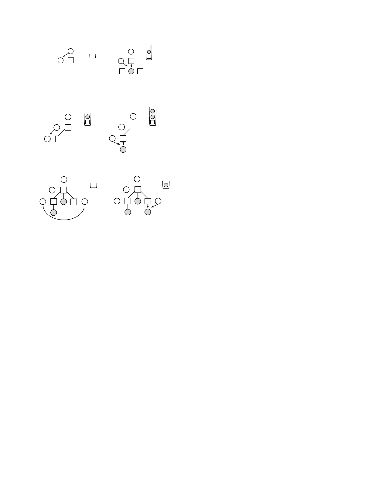
Structur ed Generativ e Models of Natural Sour ce Code Chris J. Maddison † C M A D D I S @ C S . T O RO N T O . E D U Univ ersity of T oronto Daniel T arlow D TAR L O W @ M I C RO S O F T . C O M Microsoft Research Abstract W e study the problem of building generati ve models of natural source code (NSC); that is, source code written by humans and meant to be understood by humans. Our primary con- tribution is to describe new generati v e models that are tailored to NSC. The models are based on probabilistic context free grammars (PCFGs) and neuro-probabilistic language models ( Mnih & T eh , 2012 ), which are e xtended to incorporate additional source code-specific structure. These models can be ef ficiently trained on a corpus of source code and outperform a variety of less structured baselines in terms of predicti ve log likelihoods on held-out data. 1. Introduction Source code is ubiquitous, and a great deal of human ef- fort goes into dev eloping it. An important goal is to de- velop tools that make the dev elopment of source code eas- ier , faster , and less error-prone, and to dev elop tools that are able to better understand pre-existing source code. T o date this problem has largely been studied outside of ma- chine learning. Many problems in this area do not appear to be well-suited to current machine learning technologies. Y et, source code is some of the most widely available data with many public online repositories. Additionally , mas- siv e open online courses (MOOCs) have begun to collect source code homew ork assignments from tens of thousands of students ( Huang et al. , 2013 ). At the same time, the soft- ware engineering community has recently observed that it is useful to think of source code as natural—written by hu- mans and meant to be understood by other humans ( Hindle et al. , 2012 ). This natural source code (NSC) has a great deal of statistical regularity that is ripe for study in machine learning. Pr oceedings of the 31 st International Conference on Machine Learning , Beijing, China, 2014. JMLR: W&CP volume 32. Cop y- right 2014 by the author(s). The combination of these two observ ations—the a vail- ability of data, and the presence of amenable statisti- cal structure—has opened up the possibility that machine learning tools could become useful in various tasks related to source code. At a high lev el, there are sev eral poten- tial areas of contrib utions for machine learning. First, code editing tasks could be made easier and faster . Current au- tocomplete suggestions rely primarily on heuristics dev el- oped by an Inte grated Development En vironment (IDE) de- signer . W ith machine learning methods, we might be able to offer much improved completion suggestions by le verag- ing the massiv e amount of source code av ailable in public repositories. Indeed, Hindle et al. ( 2012 ) have sho wn that ev en simple n -gram models are useful for improving code completion tools, and Nguyen et al. ( 2013 ) have extended these ideas. Other related applications include finding b ugs ( Kremenek et al. , 2007 ), mining and suggesting API us- age patterns ( Bruch et al. , 2009 ; Nguyen et al. , 2012 ; W ang et al. , 2013 ), as a basis for code complexity metrics ( Al- lamanis & Sutton , 2013 ), and to help with enforcing cod- ing con ventions ( Allamanis et al. , 2014 ). Second, machine learning might open up whole ne w applications such as au- tomatic translation between programming languages, auto- matic code summarization, and learning representations of source code for the purposes of visualization or discrim- inativ e learning. Finally , we might hope to lev erage the large amounts of existing source code to learn improved priors ov er programs for use in programming by example ( Halbert , 1984 ; Gulw ani , 2011 ) or other program induction tasks. One approach to developing machine learning tools for NSC is to improve specific one-off tasks related to source code. Indeed, much of the work cited abov e follows in this direction. An alternativ e, which we pursue here, is to dev elop a generativ e model of source code with the aim that many of the above tasks then become different forms of query on the same learned model (e.g., code comple- tion is conditional sampling; b ug fixing is model-based de- † W ork done primarily while author was an intern at Mi- crosoft Research. Structured Generati ve Models of Natural Source Code for (m[canplace] = -0; i[0] <= temp; m++) { co.nokori = Dictionary; continue; } (a) Log-bilinear PCFG for (int i = words; i < 4; ++i) { for (int j = 0; j < i; ++j) { if (words.Length % 10 == 0) { Math.Max(j+j, i*2 + Math.Abs(i+j)); } } } (b) Our Model Figure 1. Samples of for loops generated by learned models. Our model captures hierarchical structure and other patterns of vari- able usage and local scoping rules. Whitespace edited to improve readability . noising; representations may be deriv ed from latent vari- ables ( Hinton & Salakhutdinov , 2006 ) or from Fisher vec- tors ( Jaakkola & Haussler , 1998 )). W e believ e that build- ing a generativ e model focuses attention on the challenges that source code presents. It forces us to model all aspects of the code, from the high lev el structure of classes and method declarations, to constraints imposed by the pro- gramming language, to the low lev el details of how vari- ables and methods are named. W e believe building good models of NSC to be a worthwhile modelling challenge for machine learning research to embrace. In Section 2 we introduce notation and motiv ate the re- quirements of our models—they must capture the sequen- tial and hierarchical nature of NSC, naturalness, and code- specific structural constraints. In Sections 3 and 4 we in- troduce Log-bilinear T ree-T ra versal models (L TTs), which combine natural language processing models of trees with log-bilinear parameterizations, and additionally incorpo- rate compiler-like reasoning. In Section 5 we discuss how efficiently to learn these models, and in Section 7 we show empirically that they far outperform the standard NLP models that hav e previously been applied to source code. As an introductory result, Fig. 1 shows samples generated by a Probabilistic Context Free Grammar (PCFG)-based model (Fig. 1 (b)) v ersus samples generated by the full v er- sion of our model (Fig. 1 (b)). Although these models ap- ply to any common imperativ e programming language lik e C/C++/Jav a, we focus specifically on C#. This decision is based on (a) the fact that large quantities of data are read- ily av ailable online, and (b) the recently released Roslyn C# compiler ( MSDN , 2011 ) exposes APIs that allo w easy access to a rich set of internal compiler data structures and processing results. 2. Modelling Source Code In this section we discuss the challenges in building a gen- erativ e model of code. In the process we motiv ate our                      Figure 2. Example Roslyn AST . Rectangles are internal nodes and shaded circles are tokens. choice of representation and model and introduce termi- nology that will be used throughout. Hierarchical Representation. The first step in compila- tion is to lex code into a sequence of tokens , ( α t ) T t = 1 = α . T okens are strings such as “ sum ”, “. ”, or “ int ” that serve as the atomic syntactic elements of a programming language. Howe ver , representing code as a flat sequence leads to very inefficient descriptions. For example, in a C# for loop, there must be a sequence containing the tokens for , ( , an initializer statement, a condition expression, an increment statement, the token ) , then a body block. A representation that is fundamentally flat cannot compactly represent this structure, because for loops can be nested. Instead, it is more ef ficient to use the hierarchical structure that is nativ e to the programming language. Indeed, most source code processing is done on tree structures that encode this struc- ture. These trees are called abstract syntax trees (ASTs) and are constructed either explicitly or implicitly by com- pilers after lexing valid sequences of code. The leaf nodes of the AST are the tokens produced by the lex er . The inter- nal nodes { n i } N i = 1 are specific to a compiler and correspond to expressions, statements or other high le vel syntactic el- ements such as Block or ForStatement . The childr en tuple C i of an internal node n i is a tuple of nodes or to- kens. An example AST is shown in Fig. 2 . Note how the EqualsValueClause node has a subtree corresponding to the code = sum . Because many crucial properties of the source code can be deriv ed from an AST , they are a pri- mary data structure used to reason about source code. For example, the tree structure is enough to determine which variables are in scope at any point in the program. For this reason we choose the AST as the representation for source code and consider generati ve models that define distribu- tions ov er ASTs. Modelling Context Dependence. A PCFG seems like a natural choice for modelling ASTs. PCFGs generate ASTs from the root to the lea ves by repeatedly sampling children Structured Generati ve Models of Natural Source Code Algorithm 1 Sampling from L TTs. 1: initialize empty stack S 2: sample ( n , h 0 ) ∼ p ( n , h 0 ) 3: push n onto S 4: ( i , t ) ← ( 1 , 1 ) 5: while S is not empty do 6: pop the top node n from S 7: if n is an internal node then 8: n i ← n 9: sample h i ∼ p ( h i | h i − 1 ) 10: sample C i ∼ p ( C i | n i , h i ) 11: push n for n ∈ R E V E R S E D ( C i ) onto S 12: i ← i + 1 13: else 14: α t ← n 15: t ← t + 1 16: end if 17: end while tuples giv en a parent node. The procedure recurses until all leav es are tokens producing nodes n i in a depth-first trav ersal order and sampling children tuples independently of the rest of the tree. Unfortunately this independence as- sumption produces a weak model; Fig. 1 (a) sho ws samples from such a model. While basic constraints like match- ing of parentheses and braces are satisfied, most important contextual dependencies are lost. For example, identifier names (variable and method names) are drawn indepen- dently of each other giv en the internal nodes of the AST , leading to nonsense code constructions. The first source of context dependence in NSC comes from the naturalness of software. People have many stylistic habits that significantly limit the space of programs that we might expect to see. For example, when writing nested for loops, it is common to name the outer loop v ariable i and the inner loop v ariable j . The second source of conte xt de- pendence comes from additional constraints inherent in the semantics of code. Even if the syntax is context free, the fact that a program conforms to the grammar does not en- sure that a program compiles. For example, variables must be declared before they are used. Our approach to dealing with dependencies beyond what a PCFG can represent will be to introduce traversal vari- ables { h i } N i = 0 that e volv e sequentially as the nodes n i are being generated. Tra versal v ariables modulate the distrib u- tion o ver children tuples by maintaining a representation of context that depends on the state of the AST generated so far . 3. Log-bilinear T ree-T ra versal Models L TTs are a family of probabilistic models that generate ASTs in a depth-first order (Algorithm 1 ). First, the stack is initialized and the root is pushed (lines 1-4). Elements are popped from the stack until it is empty . If an internal node n i is popped (line 6), then it is expanded into a children tuple and its children are pushed onto the stack (lines 10- 11). If a token α t is popped, we label it and continue (line 14). This procedure has the effect of generating nodes in a depth-first order . In addition to the tree that is generated in a recursi ve fashion, tra versal variables h i are updated when- ev er an internal node is popped (line 9). Thus, the y trav erse the tree, ev olving sequentially , with each h i corresponding to some partial tree of the final AST . This sequential view will allow us to exploit context, such as variable scoping, at intermediate stages of the process (see Section 4 ). Algorithm 1 produces a sequence of internal nodes ( n i ) N i = 1 , trav ersal variables ( h i ) N i = 0 , and the desired tokens { α t } T t = 1 . It is defined by three distributions: (a) the prior over the root node and traversal variables, p ( n , h ) ; (b) the distribu- tion over children tuples conditioned on the parent node and h , denoted p ( C | n , h ) ; and (c) the transition distribution for the h s, denoted p ( h i | h i − 1 ) . The joint distribution ov er the elements produced by Algorithm 1 is p ( n 1 , h 0 ) N ∏ i = 1 p ( C i | n i , h i ) p ( h i | h i − 1 ) (1) Thus, L TTs can be viewed as a Markov model equipped with a stack—a special case of a Probabilistic Pushdo wn Automata (PPD A) ( Abney et al. , 1999 ). Because depth- first order produces tokens in the same order that they are observed in the code, it is particularly well-suited. W e note that other traversal orders produce valid distributions ov er trees such as right-left or breadth-first. Because we com- pare to sequential models, we consider only depth-first. Parameterizations. Most of the uncertainty in generation comes from generating children tuples. In order to a void an explosion in the number of parameters for the children tu- ple distribution p ( C | n , h ) , we use a log-bilinear form. For all distributions other than p ( C | n , h ) we use a simple tab u- lar parameterization. The log-bilinear form consists of a real-v alued vector rep- resentation of ( n i , h i ) pairs, R con ( n i , h i ) , a real-valued vec- tor representation for the children tuple, R ch ( C i ) , and a bias term for the children, b ch ( C i ) . These are combined via an inner product, which gi ves the neg ati ve energy of the chil- dren tuple − E ( C i ; n i , h i ) = R ch ( C i ) T R con ( n i , h i ) + b ch ( C i ) As is standard, this is then exponentiated and normalized to giv e the probability of sampling the children: p ( C i | n i , h i ) ∝ exp { − E ( C i ; n i , h i ) } . W e take the support over which to normalize this distribution to be the set of children tuples observed as children of nodes of type n i in the training set. The representation functions rely on the notion of an R ma- trix that can be indexed into with objects to look up D di- mensional real-valued v ectors. R x denotes the row of the R Structured Generati ve Models of Natural Source Code                                                                                                                               (a) pop n 1 , sample h 1                                                                                                                  (b) sample children, and push left-right                                                                                                                               (c) pop n 2 , sample h 2                                                                                                                          (d) sample children tuple, and push left-right                                                                                                                               (e) pop α 1 , α 2 , and n 3 , sam- ple h 3                                                                                                                          (f) sample children tuple, and push left-right Figure 3. Example sampling run from an L TT. Rectangles are in- ternal nodes, shaded circles are tokens, circles are traversal vari- ables, and stack S is shown in the state after the computations de- scribed in subcaption. Parentheses indicate tuples of nodes and ar- rows indicate conditioning. Popping of tokens omitted for brevity , but note that the y are labelled in the order encountered. matrix corresponding to an y v ariable equal to x . For exam- ple, if n i = int and n j = int , then R n i = R n j . These ob- jects may be tuples and in particular (type, int) 6 = int . Similarly , b x looks up a real number . In the simple vari- ant, each unique C sequence receiv es the representation R ch ( C i ) = R C i and b ch ( C i ) = b C i . The representations for ( n , h ) pairs are defined as sums of representations of their components. If h i is a collection of variables ( h i j represent- ing the j th v ariable at the i th step) then R con ( n i , h i ) = W con 0 R n i + H ∑ j = 1 W con j R h i j (2) The W con s are matrices (diagonal for computational effi- ciency) that modulate the contribution of a variable in a position-dependent way . In other variants the children tuple representations will also be defined as sums of their com- ponent representations. The log-bilinear parameterization has the desirable property that the number of parameters grows linearly in the dimension of h , so we can af ford to hav e high dimensional traversal variables without worry- ing about exponentially bad data fragmentation. 4. Extending L TTs The extensions of L TTs in this section allow (a) certain trav ersal variables to depend arbitrarily on previously gen- erated elements of the AST ; (b) annotating nodes with richer types; and (c) letting R ch be compositionally defined, which becomes powerful when combined with determinis- tic reasoning about variable scoping. W e distinguish between deterministic and latent traversal variables. The former can be computed deterministically from the current partial tree (the tree nodes and tokens that hav e been instantiated at step i ) that has been generated while the latter cannot. T o refer to a collection of both de- terministic and latent tra versal v ariables we continue to use the unqualified “trav ersal v ariables” term. Deterministic T raversal V ariables. In the basic genera- tiv e procedure, trav ersal variables h i satisfy the first-order Markov property , but it is possible to condition on any part of the tree that has already been produced. That is, we can replace p ( h i | h i − 1 ) by p ( h i | h 0: i − 1 , n 1: i , α 1: t ) in Eq. 1 . Inference becomes complicated unless these variables are deterministic trav ersal variables (inference is explained in Section 5 ) and the unique value that has support can be computed efficiently . Examples of these variables include the set of node types that are ancestors of a giv en node, and the last n tokens or internal nodes that ha ve been gen- erated. V ariable scoping, a more elaborate deterministic relationship, is considered later . Annotating Nodes. Other useful features may not be deterministically computable from the current partial tree. Consider kno wing that a BinaryExpression will e v aluate to an object of type int . This information can be encoded by letting nodes take values in the cross-product space of the node type space and the annotation space. For exam- ple, when adding type annotations we might hav e nodes take value ( BinaryExpression , int ) where before they were just BinaryExpression . This can be problematic, because the cardinality of the parent node space increases exponentially as we add annotations. Because the annota- tions are uncertain, this means there are more choices of node values at each step of the generative procedure, and this incurs a cost in log probabilities when ev aluating a model. Experimentally we found that simply annotating expression nodes with type information led to worse log probabilities of generating held out data: the cost of gen- erating tokens decreased because the model had access to type information, the increased cost of generating type an- notations along with nodetypes outweighed the improve- ment. Structured Generati ve Models of Natural Source Code Identifier T oken Scoping. The source of greatest uncertainty when generating a program are children of IdentifierToken nodes. IdentifierToken nodes are very common and are parents of all tokens (e.g. v ari- able and method names) that are not built-in language key- words (e.g., IntKeyword or EqualsToken ) or constants (e.g., StringLiteral s). Knowing which variables ha ve previously been declared and are currently in scope is one of the most powerful signals when predicting which IdentifierToken will be used at an y point in a program. Other useful cues include ho w recently the v ariable was de- clared and what the type the variable is. In this section we a scope model for L TTs. Scope can be represented as a set of v ariable feature vectors corresponding to each to a variable that is in scope. 1 Thus, each feature vector contains a string identifier correspond- ing to the variable along with other features as (key , v alue) tuples, for example ( type , int ) . A variable is “in scope” if there is a feature vector in the scope set that has a string identifier that is the same as the variable’ s identifier . When sampling an identifier token, there is a two step pro- cedure. First, decide whether this identifier token will be sampled from the current scope. This is accomplished by annotating each IdentifierToken internal node with a binary variable that has the states global or local . If local , proceed to use the local scope model defined next. If global , sample from a global identifier token model that giv es support to all identifier tokens. Note, we consider the global option a necessary smoothing device, although ideally we would hav e a scope model complete enough to hav e all possible identifier tokens. The scope set can be updated deterministically as we tra- verse the AST by recognizing patterns that correspond to when variables should be added or remov ed from the scope. W e implemented this logic for three cases: parameters of a method, locally declared v ariables, and class fields that hav e been defined prior in the class definition. W e do not include class fields defined after the current point in the code, and variables and methods av ailable in included namespaces. This incompleteness necessitates the global option described abov e, but these three cases are v ery com- mon and cov er many interesting cases. Giv en the scope set which contains variable feature vec- tors { v α } and parent node (IdentifierToken, local) , the probability of selecting token child α is proportional to p ( α | n i , h i ) ∝ exp { − E ( α ; n i , h i ) } , where we normalize only over the variables currently in scope. Specifically , we 1 T echnically , we vie w the scope as a deterministic traversal variable, b ut it does not contribute to R con . let R ch ( α ) and b ch ( α ) be defined as follows: R ch ( α ) = V ∑ u = 1 W ch u R v α u b ch ( α ) = V ∑ u = 1 b v α u . (3) For example, if a variable in scope has feature vector ( numNodes , ( type , int ) , ( recently-declared , 0 )), then its corresponding R ch would be a context matrix- modulated sum of representations R numNodes , R ( type , int ) , and R ( recently-declared , 0 ) . This representation will then be combined with the context representation as in the basic model. The string identifier feature numNodes is the same object as token nodes of the same string, thus they share their representation. 5. Inference and Lear ning in L TTs In this section we briefly consider how to compute gradi- ents and probabilities in L TTs. Only Deterministic T raversal V ariables. If all trav er- sal v ariables h i can be computed deterministically from the current partial tree, we use the compiler to compute the full AST corresponding to program α m . From the AST we compute the only valid setting of the trav ersal variables. Because both the AST and the traversal variables can be de- terministically computed from the token sequence, all vari- ables in the model can be treated as observed. Since L TTs are directed models, this means that the total log probability is a sum of log probabilities at each production, and learn- ing decomposes into independent problems at each produc- tion. Thus, we can simply stack all productions into a sin- gle training set and follow standard gradient-based proce- dures for training log-bilinear models. More details will be described in Section 7 , but generally we follow the Noise- Contrastiv e Estimation (NCE) technique employed in Mnih & T eh ( 2012 ). Latent T raversal V ariables. In the second case, we al- low latent trav ersal v ariables that are not deterministically computable from the AST . In this case, the traversal vari- ables couple the learning across dif ferent productions from the same tree. F or simplicity and to allo w efficient exact inference, we restrict these latent traversal v ariables to just be a single discrete variable at each step (although this re- striction could easily be lifted if one was willing to use approximate inference). Because the AST is still a deter- ministic function of the tokens, computing log probabil- ities corresponds to running the forward-backward algo- rithm over the latent states in the depth-first trav ersal of the AST . W e can formulate an EM algorithm adapted to the NCE-based learning of log-bilinear models for learning parameters. The details of this can be found in the Supple- mentary Material. Structured Generati ve Models of Natural Source Code 6. Related W ork The L TTs described here are closely related to sev eral ex- isting models. Firstly , a Hidden Markov Model (HMM) can be recovered by having all children tuples contain a token and a Next node, or just a token (which will ter- minate the sequence), and having a single discrete latent trav ersal variable. If the traversal variable has only one state and the children distributions all hav e finite support, then an L TT becomes equiv alent to a Probabilistic Context Free Grammar (PCFG). PCFGs and their v ariants are com- ponents of state-of-the-art parsers of English ( McClosky et al. , 2006 ), and many variants hav e been explored: inter- nal node annotation Charniak ( 1997 ) and latent annotations Matsuzaki et al. ( 2005 ). Aside from the question of the order of the traversals, the traversal variables make L TTs special cases of Probabilistic Pushdown Automata (PPD A) (for definition and weak equiv alence to PCFGs, see Abney et al. ( 1999 )). Log-bilinear parameterizations have been applied widely in language modeling, for n -gram models ( Saul & Pereira , 1997 ; Mnih & Hinton , 2007 ; Mnih & T eh , 2012 ) and PCFG models ( Charniak , 2000 ; Klein & Manning , 2002 ; Tito v & Henderson , 2007 ; Henderson & T itov , 2010 ). T o be clear , our claim is not that general T ree T ra versal models or the log-bilinear paremeterizations are nov el; howe ver , we believe that the full L TT construction, including the tree traversal structure, log-bilinear param- eterization, and incorporation of deterministic logic to be nov el and of general interest. The problem of modeling source code is relatively under- studied in machine learning. W e pre viously mentioned Hindle et al. ( 2012 ) and Allamanis & Sutton ( 2013 ), which tackle the same task as us but with simple NLP models. V ery recently , Allamanis & Sutton ( 2014 ) explores more sophisticated nonparametric Bayesian grammar models of source code for the purpose of learning code idioms. Liang et al. ( 2010 ) use a sophisticated non-parametric model to encode the prior that programs should factorize repeated computation, but there is no learning from existing source code, and the prior is only applicable to a functional pro- gramming language with quite simple syntax rules. Our approach builds a sophisticated and learned model and sup- ports the full language specification of a widely used imper- ativ e programming language. 7. Experimental Analysis In all experiments, we used a dataset that we collected from T opCoder .com. There are 2261 C# programs which make up 140k lines of code and 2.4M parent nodes in the col- lectiv e abstract syntax trees. These programs are solutions to programming competitions, and there is some overlap in programmers and in problems across the programs. W e created training splits based on the user identity , so the set of users in the test set are disjoint from those in the training or v alidation sets (b ut the training and v alidation sets share users). The ov erall split proportions are 20% test, 10% v al- idation, and 70% train. The e v aluation measure that we use throughout is the log probability under the model of gener- ating the full program. All logs are base 2. T o make this number more easily interpretable, we di vide by the num- ber of tokens in each program, and report the av erage log probability per token. Experimental Protocol. All experiments use a valida- tion set to choose hyperparameter values. These include the strength of a smoothing parameter and the epoch at which to stop training (if applicable). W e did a coarse grid search in each of these parameters and the numbers we re- port (for train, v alidation, and test) are all for the settings that optimized validation performance. For the gradient- based optimization, we used AdaGrad ( Duchi et al. , 2011 ) with stochastic minibatches. Unless otherwise specified, the dimension of the latent representation vectors was set to 50. Occasionally the test set will ha ve tokens or children tuples unobserved in the training set. In order to avoid as- signing zero probability to the test set, we locally smoothed ev ery children distribution with a default model that gives support to all children tuples. The numbers we report are a lower bound on the log probability of data under for a mixture of our models with this default model. Details of this smoothed model, along with additional experimental details, appear in the Supplementary Materials. There is an additional question of how to represent novel identifiers in the scope model. W e set the representations of all features in the v ariable feature vectors that were unobserved in the training set to the all zeros vector . Baselines and Basic Log-bilinear Models. The natural choices for baseline models are n -gram models and PCFG- like models. In the n -gram models we use additi ve smooth- ing, with the strength of the smoothing hyperparameter chosen to optimize validation set performance. Similarly , there is a smoothing parameter in the PCFG-like models that is chosen to optimize validation set performance. W e explored the effect of the log-bilinear parameterization in two ways. First, we trained a PCFG model that was iden- tical to the first PCFG model but with the parameteriza- tion defined using the standard log-bilinear parameteriza- tion. This is the most basic L TT model, with no trav ersal variables (L TT - / 0). The result was nearly identical to the standard PCFG. Next, we trained a 10-gram model with a standard log-bilinear parameterization, which is equiva- lent to the models discussed in ( Mnih & T eh , 2012 ). This approach dominates the basic n -gram models, allowing longer contexts and generalizing better . Results appear in Fig. 4 . Deterministic T raversal V ariables. Next, we augmented L TT - / 0 model with deterministic tra versal v ariables that in- Structured Generati ve Models of Natural Source Code Method T rain V alid T est 2-gram -4.28 -4.98 -5.13 3-gram -2.94 -5.05 -5.25 4-gram -2.70 -6.05 -6.31 5-gram -2.68 -7.22 -7.45 PCFG -3.67 -4.04 -4.23 L TT - / 0 -3.67 -4.04 -4.24 LBL 10-gram -3.19 -4.62 -4.87 Figure 4. Baseline model log probabilities per token. Method T rain V alid T est L TT - / 0 -3.67 -4.04 -4.24 L TT -Seq -2.54 -3.25 -3.46 L TT -Hi -2.28 -3.30 -3.53 L TT -HiSeq -2.10 -3.06 -3.28 Figure 5. L TT models augmented with determistically deter- minable latent variables. clude hierarchical and sequential information. The hier- archical information is the depth of a node, the kind of a node’ s parent, and a sequence of 10 ancestor history v ari- ables, which store for the last 10 ancestors, the kind of the node and the index of the child that would need to be re- cursed upon to reach the current point in the tree. The se- quential information is the last 10 tokens that were gener- ated. In Fig. 5 we report results for three v ariants: hierarchy only (L TT -Hi), sequence only (L TT -Seq), and both (L TT - HiSeq). The hierarchy features alone perform better than the sequence features alone, b ut that their contributions are independent enough that the combination of the two pro- vides a substantial gain ov er either of the indi viduals. Latent T ra versal V ariables. Next, we considered latent trav ersal variable L TT models trained with EM learning. In all cases, we used 32 discrete latent states. Here, results were more mixed. While the latent-augmented L TT (L TT - latent) outperforms the L TT - / 0 model, the gains are smaller than achiev ed by adding the deterministic features. As a baseline, we also trained a log-bilinear -parameterized stan- dard HMM, and found its performance to be far w orse than other models. W e also tried a variant where we added la- tent trav ersal variables to the L TT -HiSeq model from the previous section, but the training was too slo w to be prac- tical due to the cost of computing normalizing constants in the E step. See Fig. 6 . Scope Model. The final set of models that we trained incorporate the scope model from Section 4 (L TT -HiSeq- Scope). The features of v ariables that we use are the iden- tifier string, the type, where the variable appears in a list sorted by when the variable was declared (also known as a de Bruijn index), and where the variable appears in a list sorted by when the variable was last assigned a value. Method T rain V alid T est L TT - / 0 -3.67 -4.04 -4.24 L TT -latent -3.23 -3.70 -3.91 LBL HMM -9.61 -9.97 -10.10 Figure 6. L TT -latent models augmented with latent v ariables and learned with EM. Method T rain V alid T est L TT -HiSeq (50) -2.10 -3.06 -3.28 L TT -HiSeq-Scope (2) -2.28 -2.65 -2.78 L TT -HiSeq-Scope (10) -1.83 -2.29 -2.44 L TT -HiSeq-Scope (50) -1.54 -2.18 -2.33 L TT -HiSeq-Scope (200) -1.48 -2.16 -2.31 L TT -HiSeq-Scope (500) -1.51 -2.16 -2.32 Figure 7. L TT models with deterministic traversal variables and scope model. Number in parenthesis is the dimension of the rep- resentation vectors. Here, the additional structure provides a large additional improv ement ov er the previous best model (L TT -HiSeq). See Fig. 7 . Analysis. T o understand better where the improvements in the dif ferent models come from, and to understand where there is still room left for improvement in the models, we break down the log probabilities from the previous exper- iments based on the value of the parent node. The results appear in Fig. 8 . In the first column is the total log prob- ability number reported previously . In the next columns, the contribution is split into the cost incurred by generat- ing tok ens and trees respecti v ely . W e see, for e xample, that the full scope model pays a slightly higher cost to generate the tree structure than the Hi&Seq model, which is due to it having to properly choose whether IdentifierT okens are drawn from local or global scopes, but that it makes up for this by paying a much smaller cost when it comes to gen- erating the actual tokens. In the Supplementary Materials, we go further into the breakdowns for the best performing model, reporting the percentage of total cost that comes from the top parent kinds. IdentifierToken s from the global scope are the largest cost (30.1%), with IdentifierToken s co vered by our local scope model (10.9%) and Block s (10.6%) next. This suggests that there would be value in extending our scope model to include more IdentifierToken s and an improv ed model of Block sequences. Samples. Finally , we qualitatively ev aluate the different methods by drawing samples from the models. Samples of for loops appear in Fig. 1 . T o generate these samples, we ask (b) the PCFG and (c) the L TT -HiSeq-Scope model to generate a ForStatement . For (a) the LBL n -gram model, we simply insert a for token as the most recent token. W e also initialize the trav ersal variables to reasonable values: Structured Generati ve Models of Natural Source Code Method T otal T oken Tree L TT - / 0 -4.23 -2.78 -1.45 L TT -Seq -3.53 -2.28 -1.25 L TT -Hi -3.46 -2.18 -1.28 L TT -HiSeq -3.28 -2.08 -1.20 L TT -HiSeq-Scope -2.33 -1.10 -1.23 Figure 8. Breakdowns of test log probabilities by whether the cost came from generating the tree structure or tokens. For all models D = 50. e.g., for the L TT -HiSeq-Scope model, we initialize the lo- cal scope to include string[] words . W e also provide samples of full source code files ( CompilationUnit ) from the L TT -HiSeq-Scope model in the Supplementary Mate- rial, and additional for loops. Notice the structure that the model is able to capture, particularly related to high lev el organization, and variable use and re-use. It also learns quite subtle things, like int v ariables often appear inside square brackets. 8. Discussion Natural source code is a highly structured source of data that has been largely unexplored by the machine learning community . W e ha ve built probabilistic models that cap- ture some of the structure that appears in NSC. A key to our approach is to lev erage the great deal of work that has gone into building compilers. The result is models that not only yield large improv ements in quantitati ve measures ov er baselines, but also qualitatively produce far more re- alistic samples. There are many remaining modeling challenges. One ques- tion is how to encode the notion that the point of source code is to do something . Relatedly , how do we represent and discov er high level structure related to trying to ac- complish such tasks? There are also a number of specific sub-problems that are ripe for further study . Our model of Block statements is nai ve, and we see that it is a significant contributor to log probabilities. It would be interesting to apply more sophisticated sequence models to children tu- ples of Block s. Also, applying the compositional repre- sentation used in our scope model to other children tuples would interesting. Similarly , it would be interesting to e x- tend our scope model to handle method calls. Another high lev el piece of structure that we only briefly experimented with is type information. W e believe there to be great po- tential in properly handling typing rules, but we found that the simple approach of annotating nodes to actually hurt our models. More generally , this work’ s focus was on generative mod- eling. An observation that has become popular in machine learning lately is that learning good generati ve models can be valuable when the goal is to extract features from the data. It would be interesting to explore how this might be applied in the case of NSC. In sum, we argue that probabilistic modeling of source code provides a rich source of problems with the potential to driv e forward ne w machine learning research, and we hope that this work helps illustrate how that research might pro- ceed forward. Acknowledgments W e are grateful to John W inn, Andy Gordon, T om Minka, and Thore Graepel for helpful discussions and suggestions. W e thank Miltos Allamanis and Charles Sutton for pointers to related work. References Abney , Steven, McAllester , David, and Pereira, Fernando. Re- lating probabilistic grammars and automata. In ACL , pp. 542– 549. A CL, 1999. Allamanis, Miltiadis and Sutton, Charles. Mining source code repositories at massiv e scale using language modeling. In MSR , pp. 207–216. IEEE Press, 2013. Allamanis, Miltiadis and Sutton, Charles A. Mining idioms from source code. CoRR , abs/1404.0417, 2014. Allamanis, Miltiadis, Barr, Earl T , and Sutton, Charles. Learning natural coding conv entions. arXiv preprint , 2014. Bruch, Marcel, Monperrus, Martin, and Mezini, Mira. Learn- ing from examples to improv e code completion systems. In ESEC/FSE , pp. 213–222. A CM, 2009. Charniak, Eugene. Statistical parsing with a context-free grammar and word statistics. AAAI/IAAI , 2005:598–603, 1997. Charniak, Eugene. A maximum-entropy-inspired parser . In A CL , pp. 132–139, 2000. Duchi, John, Hazan, Elad, and Singer , Y oram. Adaptiv e subgra- dient methods for online learning and stochastic optimization. Journal of Machine Learning Research , pp. 2121–2159, 2011. Gulwani, Sumit. Automating string processing in spreadsheets using input-output e xamples. In A CM SIGPLAN Notices , vol- ume 46, pp. 317–330. A CM, 2011. Halbert, Daniel Conrad. Pr ogramming by example . PhD thesis, Univ ersity of California, Berkele y , 1984. Henderson, James and Tito v , Ivan. Incremental sigmoid belief networks for grammar learning. JMLR , 11:3541–3570, 2010. Hindle, Abram, Barr, Earl T , Su, Zhendong, Gabel, Mark, and Dev anbu, Premkumar . On the naturalness of software. In ICSE , pp. 837–847. IEEE, 2012. Hinton, Geoffre y E and Salakhutdinov , Ruslan R. Reducing the dimensionality of data with neural networks. Science , 313 (5786):504–507, 2006. Huang, Jonathan, Piech, Chris, Nguyen, Andy , and Guibas, Leonidas. Syntactic and functional variability of a million code submissions in a machine learning MOOC. In AIED , 2013. Structured Generati ve Models of Natural Source Code Jaakkola, T ommi and Haussler, David. Exploiting generative models in discriminative classifiers. In Kearns, Michael J., Solla, Sara A., and Cohn, David A. (eds.), NIPS , pp. 487–493. The MIT Press, 1998. ISBN 0-262-11245-0. Klein, Dan and Manning, Christopher D. F ast exact inference with a f actored model for natural language parsing. In NIPS , pp. 3–10, 2002. Kremenek, T ed, Ng, Andrew Y , and Engler, Dawson R. A f actor graph model for software b ug finding. In IJCAI , 2007. Liang, P ., Jordan, M. I., and Klein, D. Learning programs: A hierarchical Bayesian approach. In ICML , pp. 639–646, 2010. Matsuzaki, T akuya, Miyao, Y usuke, and Tsujii, Jun’ichi. Proba- bilistic cfg with latent annotations. In ACL , pp. 75–82. A CL, 2005. McClosky , Da vid, Charniak, Eugene, and Johnson, Mark. Effec- tiv e self-training for parsing. In ACL , pp. 152–159. A CL, 2006. Mnih, Andriy and Hinton, Geoffre y . Three ne w graphical mod- els for statistical language modelling. In ICML , pp. 641–648, 2007. Mnih, Andriy and T eh, Y ee Whye. A fast and simple algorithm for training neural probabilistic language models. In ICML , pp. 1751–1758, 2012. MSDN. Microsoft Roslyn CTP, 2011. URL http://msdn. microsoft.com/en- gb/roslyn . Nguyen, Anh T uan, Nguyen, T ung Thanh, Nguyen, Hoan Anh, T amrawi, Ahmed, Nguyen, Hung V iet, Al-K ofahi, Jafar , and Nguyen, T ien N. Graph-based pattern-oriented, context- sensitiv e source code completion. In ICSE , ICSE 2012, pp. 69–79. IEEE Press, 2012. ISBN 978-1-4673-1067-3. Nguyen, T ung Thanh, Nguyen, Anh T uan, Nguyen, Hoan Anh, and Nguyen, T ien N. A statistical semantic language model for source code. In ESEC/FSE , pp. 532–542. A CM, 2013. Saul, Lawrence and Pereira, Fernando. Aggregate and mixed- order Markov models for statistical language processing. In EMNLP , 1997. T itov , Ivan and Henderson, James. Incremental Bayesian net- works for structure prediction. In ICML , 2007. W ang, Jue, Dang, Y ingnong, Zhang, Hongyu, Chen, Kai, Xie, T ao, and Zhang, Dongmei. Mining succinct and high-coverage api usage patterns from source code. In MSR , pp. 319–328. IEEE Press, 2013. Structured Generati ve Models of Natural Source Code Supplementary Materials f or “Structur ed Generative Models of Natural Sour ce Code” EM Learning f or Latent T raversal V ariable L TTs Here we describe EM learning of L TTs with latent traversal vari- ables. Consider probability of α with deterministic trav ersal v ari- ables h d i and latent tra versal variables h l i (where h i represents the union of { h l i } and h d i ): ∑ h 0: N p ( n 1 , h 0 ) N ∏ i = 1 p ( C i | n i , h i ) p ( h l i | h l i − 1 ) × p ( h d i | h 0: i − 1 , n 1: i , , α 1: t ) (4) Firstly , the p ( h d i | · ) terms drop of f because as above we can use the compiler to compute the AST from α then use the AST to deter- ministically fill in the only legal values for the h d i variables, which makes these terms always equal to 1. It then becomes clear that the sum can be computed using the forward-backward algorithm. For learning, we follow the standard EM formulation and lo wer bound the data log probability with a free energy of the follo wing form (which for brevity drops the prior and entrop y terms): N ∑ i = 2 ∑ h l i , h l i − 1 Q i , i − 1 ( h l i , h l i − 1 ) log P ( h l i | h l i − 1 ) + N ∑ i = 1 ∑ h l i Q i ( h l i ) log p ( C i | n i , h i ) (5) In the E step, the Q’ s are updated optimally gi ven the current pa- rameters using the forward backward algorithm. In the M step, giv en Q ’ s, the learning decomposes across productions. W e rep- resent the transition probabilities using a simple tab ular represen- tation and use stochastic gradient updates. For the emission terms, it is again straightforward to use standard log-bilinear model train- ing. The only dif ference from the previous case is that there are now K training e xamples for each i , one for each possible value of h l i , which are weighted by their corresponding Q i ( h l i ) . A sim- ple way of handling this so that log-bilinear training methods can be used unmodified is to sample h l i values from the corresponding Q i ( · ) distribution, then to add unweighted examples to the train- ing set with h l i values being giv en their sampled v alue. This can then be seen as a stochastic incremental M step. More Experimental Pr otocol Details For all hyperparameters that were not validated over (such as minibatch size, scale of the random initializations, and learning rate), we chose a subsample of the training set and manually chose a setting that did best at optimizing the training log probabilities. For EM learning, we divided the data into databatches, which con- tained 10 full programs, ran forward-backward on the databatch, then created a set of minibatches on which to do an incremental M step using AdaGrad. All parameters were then held fix ed through- out the experiments, with the exception that we re-optimized the parameters for the learning that required EM, and we scaled the learning rate when the latent dimension changed. Our code used properly vectorized Python for the gradient updates and a C++ implementation of the forward-backward algorithm but was oth- erwise not particularly optimized. Run times (on a single core) ranged from a few hours to a couple days. Smoothed Model In order to avoid assigning zero probability to the test set, we as- sumed kno wledge of the set of all possible tokens, as well as all possible internal node types – information available in the Roslyn API. Nonetheless, because we specify distributions ov er tuples of children there are tuples in the test set with no support. Therefore we smooth e very p ( C i | h i , n i ) by mixing it with a def ault distribu- tion p d e f ( C i | h i , n i ) over children that gi ves broad support. p π ( C i | h i , n i ) = π p ( C i | h i , n i ) + ( 1 − π ) p d e f ( C i | h i , n i ) (6) For distributions whose children are all 1-tuples of tokens, the default model is an additiv ely smoothed model of the empiri- cal distrib ution of tok ens in the train set. For other distrib utions we model the number of children in the tuple as a Poisson dis- tribution, then model the identity of the children independently (smoothed additiv ely). This smoothing introduces trees other than the Roslyn AST with positiv e support. This opens up the possibility that there are mul- tiple trees consistent with a given token sequence and we can no longer compute log p ( α ) in the manner discussed in Section 5 . Still we report the log-probability of the AST , which is now a lower bound on log p ( α ) . Parent Kind % Log prob Count ( IdentifierToken , global ) 30.1 17518 ( IdentifierToken , local ) 10.9 27600 Block 10.6 3556 NumericLiteralToken 4.3 8070 Argument 3.6 10004 PredefinedType 3.0 7890 IfStatement 2.9 2204 AssignExpression 2.4 2747 ExpressionStatement 2.1 4141 EqualsValueClause 2.0 3937 StringLiteralToken 1.9 680 AddExpression 1.9 1882 ForStatement 1.6 1759 Figure 9. Percent of log probability contributions coming from top parent kinds for L TT -HiSeq-Scope (50) model on test set. Structured Generati ve Models of Natural Source Code for ( int i = 0 ; i < words . Length ; ++ i ) i = i . Replace ( "X" , i ) ; for ( int j = 0 ; j < words . X ; j ++ ) { if ( j [ j ] == - 1 ) continue ; if ( words [ j ] != words [ j ] ) j += thisMincost ( 1 ) ; else { j = ( j + 1 ) % 2 ; words [ j + 1 ] += words [ 0 ] ; } } for ( int j = words ; j < words . Pair ; ++ j ) for ( int i = 0 ; i < words . Length ; ++ i ) { isUpper ( i , i ) ; } for ( int i = 0 ; i < words . Length ; ++ i ) { words [ i , i ] = words . Replace ( "*" , i * 3 ) ; } for ( int j = 360 ; j < j ; ) { if ( ! words . ContainsKey ( j ) ) { if ( words . at + " " + j == j ) return ume ( j , j ) ; } else { j = 100 ; } } for ( int c = 0 ; c < c ; ++ c ) for ( int i = 0 ; i < c ; i ++ ) { if ( ! words [ i ] ) i = i ; } for ( int i = 0 ; i < words . Length ; i ++ ) { i . Parse ( i ) ; } for ( int i = words ; i < 360 ; ++ i ) { words [ i ] = words [ i ] ; i = 4 ; } Figure 10. More example for loops generated by L TT -HiSeq-Scope (50). Whitespace edited to improv e readability . Structured Generati ve Models of Natural Source Code using System ; using System . Collections . Text ; using System . Text . Text ; using System . Text . Specialized ; using kp . Specialized ; using System . Specialized . Specialized ; public class MaxFlow { public string maximalCost(int[] a, int b) { int xs = 0; int board = 0; int x = a; double tot = 100; for (int i = 0; i < xs; i++) { x = Math.mask(x); } for (int j = 0; j < x; j++) { int res = 0; if (res > 0) ++res; if (res == x) { return -1; } } for (int i = 0; i < a.Length; i++) { if (a[i - 2].Substring(board, b, xs, b, i)[i] == ’B’) x = "NO"; else if (i == 3) { if (i > 1) { x = x.Abs(); } else if (a[i] == ’Y’) return "NO"; } for (int j = 0; j < board; j++) if (j > 0) board[i] = j.Parse(3); } long[] x = new int[a.Count]; int[] dp = board; for (int k = 0; k < 37; k++) { if (x.Contains < x.Length) { dp[b] = 1000000; tot += 1; } if (x[k, k] < k + 2) { dp = tot; } } return "GREEN"; } } Figure 11. Example CompilationUnit generated by L TT -HiSeq-Scope (50). Whitespace edited to improv e readability . Structured Generati ve Models of Natural Source Code using System ; using System . sampling . Specialized ; public class AlternatingLane { public int count = 0 ; int dc = { 0 , 0 , 0 , 0 } ; double suma = count . Reverse ( count ) ; public int go ( int ID , int To , int grape , string [ ] next ) { if ( suma == 1000 || next . StartsWith . To ( ID ) [ To ] == next [ To ] ) return ; if ( next [ next ] != - 1 ) { next [ To , next ] = 1010 ; Console . Add ( ) ; } for ( int i = 0 ; i < ( 1 << 10 ) ; i ++ ) { if ( i == dc ) NextPerm ( i ) ; else { count ++ ; } } return div ( next ) + 1 ; } string solve ( string [ ] board ) { if ( board [ count ] == ’1’ ) { return 10 ; } return suma ; } } Figure 12. Example CompilationUnit generated by L TT -HiSeq-Scope (50). Whitespace edited to improv e readability . Structured Generati ve Models of Natural Source Code using System ; using System . Collections . Collections ; using System . Collections . Text ; using System . Text . Text ; public class TheBlackJackDivTwo { int dp = 2510 ; int vx = new int [ ] { - 1 , 1 , 1 , 2 } ; int [ ] i ; int cs ; double xy ; int pack2 ; long getlen ( char tree ) { return new bool [ 2 ] ; } int getdist ( int a , int splitCost ) { if ( ( ( 1 << ( a + vx ) ) + splitCost . Length + vx ) != 0 ) i = splitCost * 20 + splitCost + ( splitCost * ( splitCost [ a ] - i [ splitCost ] ) ) ; int total = i [ a ] ; for ( int i = 0 ; i < pack2 ; i ++ ) { if ( can ( 0 , i , a , i , i ) ) { total [ a ] = true ; break ; } i [ i ] -= i [ a ] ; total = Math . CompareTo ( ) ; saiki1 ( a , vx , a , i ) ; } return total + 1 < a && splitCost < a ; } } Figure 13. Example CompilationUnit generated by L TT -HiSeq-Scope (50). Whitespace edited to improv e readability .