Asymptotically Exact, Embarrassingly Parallel MCMC

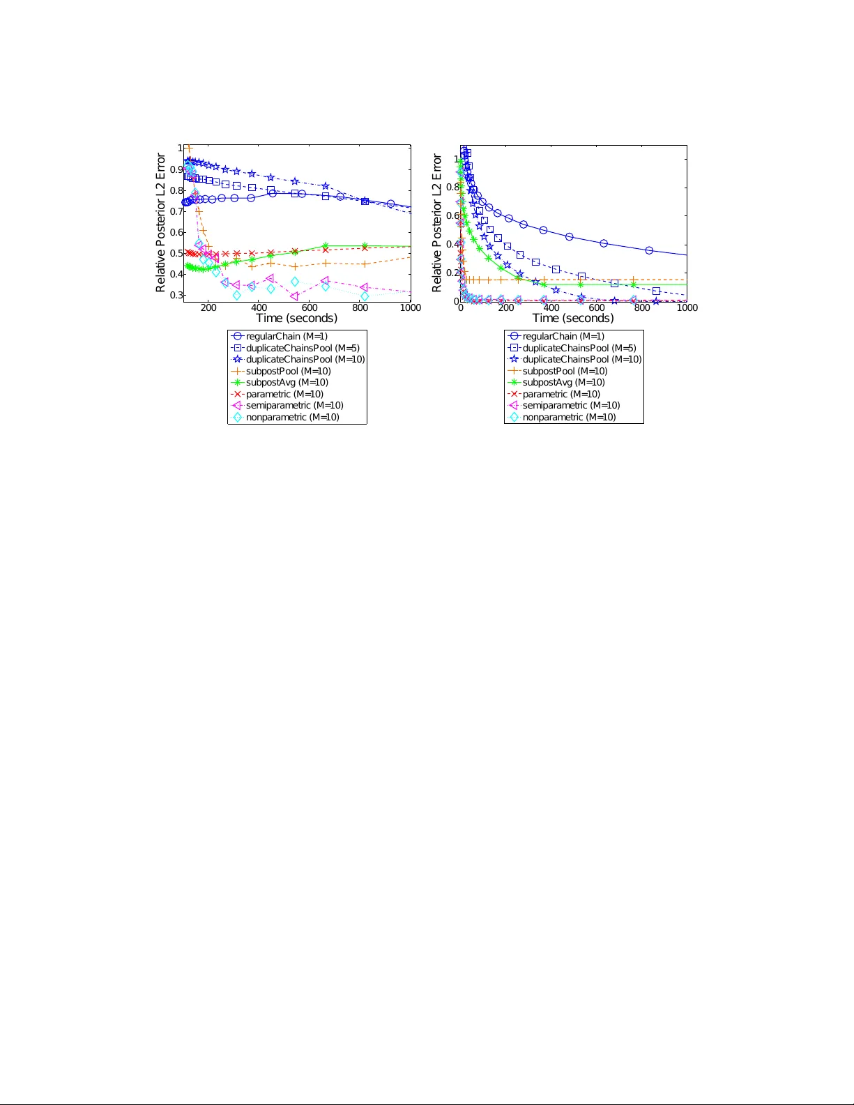
Asymptotically Exact, Em barrassingly P arallel MCMC Willie Neisw anger 1 , Chong W ang 2 , and Eric Xing 3 Machine L e arning Dep artment, Carne gie Mel lon University Abstract. Comm unication costs, resulting from synchronization requiremen ts during learning, can greatly slo w down man y parallel machine learning algorithms. In this pap er, we presen t a parallel Mark ov c hain Monte Carlo (MCMC) algorithm in which subsets of data are processed indep endently , with very little comm unication. First, w e arbitrarily partition data onto multiple mac hines. Then, on each mac hine, an y classical MCMC metho d (e.g., Gibbs sampling) may be used to dra w samples from a p osterior distribution given the data subset. Finally , the samples from each mac hine are com bined to form samples from the full p osterior. This embarrassingly parallel algorithm allows eac h machine to act indep endently on a subset of the data (without comm unication) until the final combination stage. W e prov e that our algorithm generates asymptotically exact samples and empirically demonstrate its abilit y to parallelize burn-in and sampling in several models. 1. Introduction Mark ov chain Mon te Carlo (MCMC) methods are p opular to ols for p erforming approximate Ba yesian inference via posterior sampling. One ma jor b enefit of these techniques is that they guaran tee asymptotically exact reco very of the p osterior distribution as the num b er of posterior samples grows. Ho wev er, MCMC metho ds ma y tak e a prohibitively long time, since for N data points, most metho ds must p erform O ( N ) op erations to draw a sample. F urthermore, MCMC methods might require a large num ber of “burn-in” steps b efore beginning to generate represen tative samples. F urther complicating matters is the issue that, for many big data applications, it is necessary to store and pro cess data on multiple mac hines, and so MCMC m ust b e adapted to run in these data-distributed settings. Researc hers currently tackle these problems indep endently , in t wo primary wa ys. T o sp eed up sampling, multiple indep endent chains of MCMC can be run in parallel [ 20 , 11 , 13 ]; how ever, eac h c hain is still run on the en tire dataset, and there is no sp eed-up of the burn-in pro cess (as eac h c hain m ust still complete the full burn-in b efore generating samples). T o run MCMC when data is partitioned among m ultiple machines, each mac hine can perform computation that in volv es a subset of the data and exchange information at eac h iteration to dra w a sample [ 10 , 14 , 18 ]; how ever, this requires a significan t amoun t of communication b etw een machines, whic h can greatly increase computation time when machines wait for external information [ 1 , 7 ]. W e aim to develop a pro cedure to tac kle b oth problems simultaneously , to allow for quick er burn-in and sampling in settings where data are partitioned among machines. T o accomplish this, we propose the follo wing: on each mac hine, run MCMC on only a subset of the data (indep enden tly , without comm unication betw een mac hines), and then combine the samples from eac h machine to algorithmically construct samples from the full-data p osterior distribution. W e’d lik e our procedure to satisfy the following four criteria: (1) Each machine only has access to a p ortion of the data. (2) Eac h machine p erforms MCMC indep endently , without comm unicating (i.e. the pro ce- dure is “embarrassingly parallel”). 1 willie@cs.cmu.edu , 2 chongw@cs.princeton.edu , 3 epxing@cs.cmu.edu . Last revised March 24, 2014. 1 2 WILLIE NEISW ANGER, CHONG W ANG, AND ERIC XING (3) Each machine can use an y type of MCMC to generate samples. (4) The combination pro cedure yields prov ably asymptotically exact samples from the full-data posterior. The third criterion allows existing MCMC algorithms or softw are pac k ages to b e run directly on subsets of the data—the com bination procedure then acts as a p ost-pro cessing step to transform the samples to the correct distribution. Note that this pro cedure is particularly suitable for use in a MapReduce [ 4 ] framew ork. Also note that, unlik e current strategies, this pro cedure does not in volv e m ultiple “duplicate” chains (as each chain uses a different p ortion of the data and samples from a differen t p osterior distribution), nor do es it inv olve parallelizing a single chain (as there are multiple chains op erating independently). W e will sho w ho w this allo ws our metho d to, in fact, parallelize and greatly reduce the time required for burn-in. In this paper we will (1) introduce and define the subp osterior density—a modified p osterior giv en a subset of the data—which will be used hea vily , (2) presen t methods for the em barrassingly parallel MCMC and com bination pro cedure, (3) prov e theoretical guaran tees ab out the samples generated from our algorithm, (4) describ e the curren t scop e of the presented metho d (i.e. where and when it can b e applied), and (5) show empirical results demonstrating that we can achiev e sp eed-ups for burn-in and sampling while meeting the ab ov e four criteria. 2. Embarrassingl y P arallel MCMC The basic idea b ehind our method is to partition a set of N i.i.d. data p oints x N = { x 1 , · · · , x N } in to M subsets, sample from the subp osterior —the p osterior given a data subset with an underweigh ted prior—in parallel, and then combine the resulting samples to form samples from the full-data posterior p ( θ | x N ), where θ ∈ R d and p ( θ | x N ) ∝ p ( θ ) p ( x N | θ ) = p ( θ ) Q N i =1 p ( x i | θ ). More formally , given data x N partitioned in to M subsets { x n 1 , . . . , x n M } , the pro cedure is: (1) F or m = 1 , . . . , M (in parallel): Sample from the subp osterior p m , where p m ( θ ) ∝ p ( θ ) 1 M p ( x n m | θ ) . (2.1) (2) Com bine the subp osterior samples to pro duce samples from an estimate of the sub- p osterior density pro duct p 1 ··· p M , which is prop ortional to the full-data posterior, i.e. p 1 ··· p M ( θ ) ∝ p ( θ | x N ). W e w ant to emphasize that w e do not need to iterate o ver these steps and the combination stage (step 3) is the only step that requires comm unication b et ween machines. Also note that sampling from each subp osterior (step 2) can typically b e done in the same w ay as one w ould sample from the full-data p osterior. F or example, when using the Metrop olis-Hastings algorithm, one w ould compute the likelihoo d ratio as p ( θ ∗ ) 1 M p ( x n m | θ ∗ ) p ( θ ) 1 M p ( x n m | θ ) instead of p ( θ ∗ ) p ( x N | θ ∗ ) p ( θ ) p ( x N | θ ) , where θ ∗ is the proposed mov e. In the next section, w e show how the combination stage (step 3) is carried out to generate samples from the full-data p osterior using the subp osterior samples. 3. Combining Subposterior Samples Our general idea is to com bine the subp osterior samples in suc h a wa y that w e are implicitly sampling from an estimate of the subp osterior density pro duct function \ p 1 ··· p M ( θ ). If our densit y pro duct estimator is consistent, then we can sho w that w e are dra wing asymptotically exact samples from the full posterior. F urther, b y studying the estimator error rate, we can explicitly analyze ho w quic kly the distribution from which we are dra wing samples is con verging to the true p osterior (and th us compare differen t com bination algorithms). ASYMPTOTICALL Y EXA CT, EMBARRASSINGL Y P ARALLEL MCMC 3 In the following three sections we presen t pro cedures that yield samples from differen t estimates of the density pro duct. Our first example is based on a simple parametric estimator motiv ated by the Bernstein-von Mises theorem [ 12 ]; this pro cedure generates approximate (asymptotically biased) samples from the full p osterior. Our second example is based on a nonparametric estimator, and produces asymptotically exact samples from the full posterior. Our third example is based on a semiparametric estimator, which combines b eneficial asp ects from the previous tw o estimators while also generating asymptotically exact samples. 3.1. Approximate posterior sampling with a parametric estimator The first metho d for forming samples from the full p osterior given subp osterior samples in volv es using an approximation based on the Bernstein-von Mises (Bay esian central limit) theorem, an imp ortant result in Bay esian asymptotic theory . Assuming that a unique, true data-generating mo del exists and is denoted θ 0 , this theorem states that the p osterior tends to a normal distribution concen trated around θ 0 as the n umber of observ ations grows. In particular, under suitable regularit y conditions, the p osterior P ( θ | x N ) is w ell approximated by N d ( θ 0 , F − 1 N ) (where F N is the fisher information of the data) when N is large [ 12 ]. Since w e aim to p erform p osterior sampling when the n umber of observ ations is large, a normal parametric form often serv es as a goo d p osterior approximation. A similar appro ximation was used in [ 2 ] in order to facilitate fast, appro ximately correct sampling. W e therefore estimate each subp osterior density with b p m ( θ ) = N d ( θ | b µ m , b Σ m ) where b µ m and b Σ m are the sample mean and co v ariance, resp ectiv ely , of the subp osterior samples. The pro duct of the M subp osterior densities will b e prop ortional to a Gaussian p df, and our estimate of the densit y pro duct function p 1 ··· p M ( θ ) ∝ p ( θ | x N ) is \ p 1 ··· p M ( θ ) = b p 1 ··· b p M ( θ ) ∝ N d  θ | b µ M , b Σ M  , where the parameters of this distribution are b Σ M = M X m =1 b Σ − 1 m ! − 1 (3.1) b µ M = b Σ M M X m =1 b Σ − 1 m b µ m ! . (3.2) These parameters can be computed quickly and, if desired, online (as new subp osterior samples arriv e). 3.2. Asymptotically exact p osterior sampling with nonparametric density pro duct estimation In the previous method we made a parametric assumption based on the Bernstein-v on Mises theorem, which allows us to generate appro ximate samples from the full p osterior. Although this parametric estimate has quick conv ergence, it generates asymptotically biased samples, esp ecially in cases where the p osterior is particularly non-Gaussian. In this section, we develop a pro cedure that implicitly samples from the pro duct of nonparametric densit y estimates, which allo ws us to pro duce asymptotically exact samples from the full p osterior. By constructing a consisten t density pro duct estimator from which we can generate samples, w e ensure that the distribution from which we are sampling con verges to the full posterior. 4 WILLIE NEISW ANGER, CHONG W ANG, AND ERIC XING Giv en T samples 1 { θ m t m } T t m =1 from a subposterior p m , w e can write the k ernel densit y estimator b p m ( θ ) as, b p m ( θ ) = 1 T T X t m =1 1 h d K  k θ − θ m t m k h  = 1 T T X t m =1 N d ( θ | θ m t m , h 2 I d ) , where we hav e used a Gaussian kernel with bandwidth parameter h . After we hav e obtained the kernel density estimator b p m ( θ ) for M subp osteriors, we define our nonparametric density pro duct estimator for the full posterior as \ p 1 ··· p M ( θ ) = b p 1 ··· b p M ( θ ) = 1 T M M Y m =1 T X t m =1 N d ( θ | θ m t m , h 2 I d ) ∝ T X t 1 =1 ··· T X t M =1 w t · N d  θ    ¯ θ t · , h 2 M I d  . (3.3) This estimate is the probability density function (p df ) of a mixture of T M Gaussians with unnormalize d mixture weigh ts w t · . Here, w e use t · = { t 1 , . . . , t M } to denote the set of indices for the M samples { θ 1 t 1 , . . . , θ M t M } (eac h from a separate machine) asso ciated with a given mixture comp onen t, and w e define ¯ θ t · = 1 M M X m =1 θ m t m (3.4) w t · = M Y m =1 N d  θ m t m | ¯ θ t · , h 2 I d  . (3.5) Although there are T M p ossible mixture comp onen ts, w e can efficien tly generate samples from this mixture by first sampling a mixture comp onent (based on its unnormalized comp onen t w eight w t · ) and then sampling from this (Gaussian) comp onen t. In order to sample mixture comp onen ts, we use an indep endent Metrop olis within Gibbs (IMG) sampler. This is a form of MCMC, where at eac h step in the Mark ov chain, a single dimension of the current state is prop osed (i.e. sampled) independently of its current v alue (while keeping the other dimensions fixed) and then is accepted or rejected. In our case, at each step, a new mixture component is prop os ed by redrawing one of the M curren t sample indices t m ∈ t · asso ciated with the comp onen t uniformly and then accepting or rejecting the resulting prop osed comp onent based on its mixture w eigh t. W e giv e the IMG algorithm for com bining subp osterior samples in Algorithm 1. 2 In certain situations, Algorithm 1 may hav e a lo w acceptance rate and therefore ma y mix slo wly . One wa y to remedy this is to p erform the IMG combination algorithm multiple times, b y first applying it to groups of ˜ M < M subp osteriors and then applying the algorithm again to the output samples from eac h initial application. F or example, one could b egin by applying the algorithm to all M 2 pairs (leaving one subp osterior alone if M is o dd), then rep eating this 1 F or ease of description, we assume eac h mac hine generates the same n umber of samples, T . In practice, they do not hav e to be the same. 2 Again for simplicit y , we assume that we generate T samples to represen t the full posterior, where T is the num ber of subp osterior samples from eac h mac hine. ASYMPTOTICALL Y EXA CT, EMBARRASSINGL Y P ARALLEL MCMC 5 pro cess—forming pairs and applying the combination algorithm to pairs only—until there is only one set of samples remaining, which are samples from the density pro duct estimate. Algorithm 1 Asymptotically Exact Sampling via Nonparametric Density Pro duct Estimation Input: Subp osterior samples: { θ 1 t 1 } T t 1 =1 ∼ p 1 ( θ ) , . . . , { θ M t M } T t M =1 ∼ p M ( θ ) Output: Posterior samples (asymptotically , as T → ∞ ): { θ i } T i =1 ∼ p 1 ··· p M ( θ ) ∝ p ( θ | x N ) 1: Draw t · = { t 1 , . . . , t M } iid ∼ Unif( { 1 , . . . , T } ) 2: for i = 1 to T do 3: Set h ← i − 1 / (4+ d ) 4: for m = 1 to M do 5: Set c · ← t · 6: Dra w c m ∼ Unif( { 1 , . . . , T } ) 7: Dra w u ∼ Unif([0 , 1]) 8: if u < w c · /w t · then 9: Set t · ← c · 10: end if 11: end for 12: Dra w θ i ∼ N d ( ¯ θ t · , h 2 M I d ) 13: end for 3.3. Asymptotically exact p osterior sampling with semiparametric density pro duct estimation Our first example made use of a parametric estimator, whic h has quick conv ergence, but may b e asymptotically biased, while our second example made use of a nonparametric estimator, whic h is asymptotically exact, but may conv erge slowly when the n umber of dimensions is large. In this example, w e implicitly sample from a semiparametric density pro duct estimate, whic h allo ws us to lev erage the fact that the full p osterior has a near-Gaussian form when the num b er of observ ations is large, while still pro viding an asymptotically unbiased estimate of the p osterior densit y , as the n umber of subposterior samples T → ∞ . W e make use of a semiparametric densit y estimator for p m that consists of the pro duct of a parametric estimator b f m ( θ ) ( in our case N d ( θ | b µ m , b Σ m ) as abov e ) and a nonparametric estimator b r ( θ ) of the correction function r ( θ ) = p m ( θ ) / b f m ( θ ) [ 6 ]. This estimator gives a near- Gaussian estimate when the n umber of samples is small, and conv erges to the true density as the n umber of samples grows. Giv en T samples { θ m t m } T t m =1 from a subp osterior p m , we can write the estimator as b p m ( θ ) = b f m ( θ ) b r ( θ ) = 1 T T X t m =1 1 h d K  k θ − θ m t m k h  b f m ( θ ) b f m ( θ m t m ) = 1 T T X t m =1 N d ( θ | θ m t m , h 2 I d ) N d ( θ | b µ m , b Σ m ) N d ( θ m t m | b µ m , b Σ m ) , where we hav e used a Gaussian k ernel with bandwidth parameter h for the nonparametric comp onen t of this estimator. Therefore, we define our semiparametric density pro duct estimator 6 WILLIE NEISW ANGER, CHONG W ANG, AND ERIC XING to be \ p 1 ··· p M ( θ ) = b p 1 ··· b p M ( θ ) = 1 T M M Y m =1 T X t m =1 N d ( θ | θ m t m , hI d ) N d ( θ | b µ m , b Σ m ) h d N d ( θ m t m | b µ m , b Σ m ) ∝ T X t 1 =1 ··· T X t M =1 W t · N d ( θ | µ t · , Σ t · ) . This estimate is prop ortional to the p df of a mixture of T M Gaussians with unnormalized mixture w eights, W t · = w t · N d  ¯ θ t · | b µ M , b Σ M + h M I d  Q M m =1 N d ( θ m t m | b µ m , b Σ m ) , where ¯ θ t · and w t · are given in Eqs. 3.4 and 3.5. W e can write the parameters of a giv en mixture comp onen t N d ( θ | µ t · , Σ t · ) as Σ t · =  M h I d + b Σ − 1 M  − 1 , µ t · = Σ t ·  M h I d ¯ θ t · + b Σ − 1 M b µ M  , where b µ M and b Σ M are giv en by Eq. 3.1 and 3.2. W e can sample from this semiparametric estimate using the IMG procedure outlined in Algorithm 1, replacing the comp onent weigh ts w t · with W t · and the comp onent parameters ¯ θ t · and h M I d with µ t · and Σ t · . W e also hav e a second semiparametric procedure that ma y giv e higher acceptance rates in the IMG algorithm. W e follow the abov e semiparametric procedure, where eac h comp onent is a normal distribution with parameters µ t · and Σ t · , but we use the nonparametric comp onent w eights w t · instead of W t · . This pro cedure is also asymptotically exact, since the semiparametric comp onen t parameters µ t · and Σ t · approac h the nonparametric comp onent parameters ¯ θ t · and h M I d as h → 0, and thus this pro cedure tends to the nonparametric procedure given in Algorithm 1. 4. Method Complexity Giv en M data subsets, to pro duce T samples in d dimensions with the nonparametric or semiparametric asymptotically exact pro cedures (Algorithm 1) requires O ( dT M 2 ) op erations. The v ariation on this algorithm that performs this pro cedure M − 1 times on pairs of subp osteriors (to increase the acceptance rate; detailed in Section 3.2) instead requires only O ( dT M ) operations. W e ha ve presented our method as a tw o step pro cedure, where first parallel MCMC is run to completion, and then the com bination algorithm is applied to the M sets of samples. W e can instead perform an online version of our algorithm: as eac h machine generates a sample, it immediately sends it to a master mac hine, which combines the incoming samples 3 and performs the accept or reject step (Algorithm 1, lines 3-12). This allo ws the parallel MCMC phase and the com bination phase to be p erformed in parallel, and do es not require transfering large volumes of data, as only a single sample is ever transferred at a time. The total comm unication required b y our metho d is transferring O ( dT M ) scalars ( T samples from each of M mac hines), and as stated ab ov e, this can b e done online as MCMC is b eing 3 F or the semiparametric metho d, this will inv olve an online update of mean and v ariance Gaussian parameters. ASYMPTOTICALL Y EXA CT, EMBARRASSINGL Y P ARALLEL MCMC 7 carried out. F urther, the communication is unidirectional, and eac h machine do es not pause and w ait for an y information from other machines during the parallel sampling pro cedure. 5. Theoretical Resul ts Our second and third pro cedures aim to draw asymptotically exact samples by sampling from (fully or partially) nonparametric estimates of the density pro duct. W e prov e the asymptotic correctness of our estimators, and b ound their rate of con vergence. This will ensure that w e are generating asymptotically correct samples from the full p osterior as the num b er of samples T from eac h subp osterior gro ws. 5.1. Density product estimate conv ergence and risk analysis T o pro ve (mean-square) consistency of our estimator, w e give a b ound on the mean-squared error (MSE), and show that it tends to zero as we increase the n umber of samples dra wn from eac h subp osterior. T o pro ve this, w e first bound the bias and v ariance of the estimator. The follo wing pro ofs make use of similar b ounds on the bias and v ariance of the nonparametric and semiparametric densit y estimators, and therefore the theory applies to b oth the nonparametric and semiparametric density pro duct estimators. Throughout this analysis, w e assume that we ha ve T samples { θ m t m } T t m =1 ⊂ X ⊂ R d from each subp osterior ( m = 1 , . . . , M ), and that h ∈ R + denotes the bandwidth of the nonparametric densit y pro duct estimator (which is annealed to zero as T → ∞ in Algorithm 1). Let H¨ older class Σ( β , L ) on X b e defined as the set of all ` = b β c times differen tiable functions f : X → R whose deriv ative f ( l ) satisfies | f ( ` ) ( θ ) − f ( ` ) ( θ 0 ) | ≤ L | θ − θ 0 | β − ` for all θ , θ 0 ∈ X . W e also define the class of densities P ( β , L ) to be P ( β , L ) =  p ∈ Σ( β , L )    p ≥ 0 , Z p ( θ ) dθ = 1  . W e also assume that all subp osterior densities p m are b ounded, i.e. that there exists some b > 0 suc h that p m ( θ ) ≤ b for all θ ∈ R d and m ∈ { 1 , . . . , M } . First, w e b ound the bias of our estimator. This sho ws that the bias tends to zero as the bandwidth shrinks. Lemma 5.1. The bias of the estimator \ p 1 ··· p M ( θ ) satisfies sup p 1 ,...,p M ∈P ( β ,L )   E  \ p 1 ··· p M ( θ )  − p 1 ··· p M ( θ )   ≤ M X m =1 c m h mβ for some c 1 , . . . , c M > 0 . Pr o of. F or all p 1 , . . . , p M ∈ P ( β , L ), | E  \ p 1 ··· p M  − p 1 ··· p M | = | E [ b p 1 ··· b p M ] − p 1 ··· p M | = | E [ b p 1 ] ··· E [ b p M ] − p 1 ··· p M | ≤   ( p 1 + ˜ c 1 h β ) ··· ( p M + ˜ c M h β ) − p 1 ··· p M   ≤   c 1 h β + . . . + c M h M β   ≤   c 1 h β   + . . . +   c M h M β   = M X m =1 c m h mβ 8 WILLIE NEISW ANGER, CHONG W ANG, AND ERIC XING where w e ha ve used the fact that | E [ c p m ] − p | ≤ ˜ c m h β for some ˜ c m > 0.  Next, w e b ound the v ariance of our estimator. This sho ws that the v ariance tends to zero as the n umber of samples grows large and the bandwidth shrinks. Lemma 5.2. The varianc e of the estimator \ p 1 ··· p M ( θ ) satisfies sup p 1 ,...,p M ∈P ( β ,L ) V  \ p 1 ··· p M ( θ )  ≤ M X m =1  M m  c m T m h dm for some c 1 , . . . , c M > 0 and 0 < h ≤ 1 . Pr o of. F or all p 1 , . . . , p M ∈ P ( β , L ), V [ \ p 1 ··· p M ] = E  b p 2 1  ··· E  b p 2 M  − E [ b p 1 ] 2 ··· E [ b p M ] 2 = M Y m =1 V [ b p m ] + E [ b p m ] 2 ! − M Y m =1 E [ b p m ] 2 ! ≤ M − 1 X m =0  M m  ˜ c m c M − m T M − m h d ( M − m ) ≤ M X m =1  M m  c m T m h dm where we hav e used the facts that V [ b p m ] ≤ c T h d for some c > 0 and E [ b p m ] 2 ≤ ˜ c for some ˜ c > 0.  Finally , w e use the bias and v ariance bounds to b ound the MSE, which shows that our estimator is consistent. Theorem 5.3. If h  T − 1 / (2 β + d ) , the me an-squar e d err or of the estimator \ p 1 ··· p M ( θ ) satisfies sup p 1 ,...,p M ∈P ( β ,L ) E  Z  \ p 1 ··· p M ( θ ) − p 1 ··· p M ( θ )  2 dθ  ≤ c T 2 β / (2 β + d ) for some c > 0 and 0 < h ≤ 1 . Pr o of. F or all p 1 , . . . , p M ∈ P ( β , L ), using the fact that the mean-squared error is equal to the v ariance plus the bias squared, we hav e that E  Z  \ p 1 ··· p M ( θ ) − p 1 ··· p M ( θ )  2 dθ  ≤ M X m =1 c m h mβ ! 2 + M X m =1  M m  ˜ c m T m h dm ≤ k T − 2 β / (2 β + d ) + ˜ k T 1 − d (2 β + d ) (for some k , ˜ k > 0) ≤ c T 2 β / (2 β + d ) for some c 1 , . . . , c M > 0 and ˜ c 1 , . . . , ˜ c M > 0.  6. Method Scope The theoretical results and algorithms in this pap er hold for p osterior distributions ov er finite-dimensional real spaces. These include generalized linear mo dels (e.g. linear, logistic, or Poisson regression), mixture mo dels with kno wn w eights, hierarchical mo dels, and (more generally) finite-dimensional graphical mo dels with unconstrained v ariables. This also includes ASYMPTOTICALL Y EXA CT, EMBARRASSINGL Y P ARALLEL MCMC 9 b oth unimodal and m ultimo dal posterior densities (suc h as in Section 8.2). Ho wev er, the metho ds and theory presen ted here do not y et extend to cases suc h as infinite dimensional mo dels (e.g. nonparametric Bay esian mo dels [ 5 ]) nor to distributions o ver the simplex (e.g. topics in laten t Dirichlet allo cation [ 3 ]). In the future, w e hop e to extend this work to these domains. 7. Rela ted W ork In [ 19 , 2 , 16 ], the authors develop a w a y to sample approximately from a posterior distribution when only a small randomized mini-batch of data is used at eac h step. In [ 9 ], the authors used a hypothesis test to decide whether to accept or reject prop osals using a small set of data (adaptiv ely) as opp osed to the exact Metrop olis-Hastings rule. This reduces the amount of time required to compute the acceptance ratio. Since all of these algorithms are still sequential, they can be directly used in our algorithm to generate subp osterior samples to further speed up the en tire sampling pro cess. Sev eral parallel MCMC algorithms hav e b een designed for sp ecific mo dels, such as for topic models [ 18 , 14 ] and nonparametric mixture mo dels [ 21 ]. These approaches still require sync hronization to b e correct (or approximately correct), while ours aims for more general mo del settings and do es not need sync hronization un til the final com bination stage. Consensus Mon te Carlo [ 17 ] is perhaps the most relev ant work to ours. In this algorithm, data is also p ortioned into different machines and MCMC is p erformed indep endently on each mac hine. Thus, it roughly has the same time complexity as our algorithm. Ho wev er, the prior is not explicitly rew eighted during sampling as we do in Eq 2.1, and final samples for the full p osterior are generated by av eraging subp osterior samples. F urthermore, this algorithm has few theoretical guaran tees. W e find that this algorithm can be viewed as a relaxation of our nonparametric, asymptotically exact sampling pro cedure, where samples are generated from an ev enly weigh ted mixture (instead of eac h comp onent having weigh t w t · ) and where eac h sample is set to ¯ θ t · instead of b eing drawn from N  ¯ θ t · , h M I d  . This algorithm is one of our exp erimental baselines. 8. Empirical Study In the follo wing sections, we demonstrate empirically that our metho d allows for quick er, MCMC-based estimation of a p osterior distribution, and that our consistent-estimator-based pro cedures yield asymptotically exact results. W e show our metho d on a few Bay esian models using b oth syn thetic and real data. In each exp eriment, w e compare the following strategies for parallel, comm unication-free sampling: 4 • Single c hain full-data posterior samples ( regularChain )—T ypical, single-chain MCMC for sampling from the full-data p osterior. • Parametric subp osterior densit y pro duct estimate ( parametric )—F or M sets of subposterior samples, the combination yielding samples from the parametric density pro duct estimate. • Nonparametric subp osterior density pro duct estimate ( nonparametric )—F or M sets of subposterior samples, the combination yielding samples from the nonparametric densit y pro duct estimate. • Semiparametric subp osterior density product estimate ( semiparametric )—F or M sets of subp osterior samples, the combination yielding samples from the semipara- metric densit y pro duct estimate. 4 W e did not directly compare with the algorithms that require synchronization since the setup of these experiments can b e rather different. W e plan to explore these comparisons in the extended version of this paper. 10 WILLIE NEISW ANGER, CHONG W ANG, AND ERIC XING • Subp osterior sample a verage ( subpostAvg )—F or M sets of subposterior samples, the a verage of M samples consisting of one sample tak en from each subp osterior. • Subp osterior sample p o oling ( subpostPool )—F or M sets of subposterior samples, the union of all sets of samples. • Duplicate c hains full-data p osterior sample p o oling ( duplicateChainsPool )— F or M sets of samples from the full-data p osterior, the union of all sets of samples. T o assess the p erformance of our sampling and combination strategies, w e ran a single c hain of MCMC on the full data for 500,000 iterations, remov ed the first half as burn-in, and considered the remaining samples the “groundtruth” samples for the true p osterior densit y . W e then needed a general metho d to compare the distance b et ween tw o densities given samples from each, which holds for general densities (including m ultimo dal densities, where it is ineffective to compare momen ts such as the mean and v ariance 5 ). F ollowing work in density-based regression [ 15 ], w e use an estimate of the L 2 distance, d 2 ( p, ˆ p ), betw een the groundtruth p osterior densit y p and a prop osed posterior density b p , where d 2 ( p, ˆ p ) = k p − b p k 2 =  R ( p ( θ ) − b p ( θ )) 2 dθ  1 / 2 . In the following exp erimen ts in volving timing, to compute the p osterior L 2 error at each time p oin t, we collected all samples generated b efore a giv en num ber of seconds, and added the time tak en to transfer the samples and combine them using one of the proposed metho ds. In all exp erimen ts and metho ds, w e follo wed a fixed rule of removing the first 1 6 samples for burn-in (whic h, in the case of combination pro cedures, was applied to eac h set of subp osterior samples b efore the combination was p erformed). Exp erimen ts were conducted with a standard cluster system. W e obtained subp osterior samples b y submitting batc h jobs to each work er since these jobs are all indep endent. W e then sa ved the results to the disk of each work er and transferred them to the same machine which p erformed the final combination. 8.1. Generalized Linear Mo dels Generalized linear mo dels are widely used for man y regression and classification problems. Here we conduct exp eriments, using logistic regression as a test case, on both synthetic and real data to demonstrate the sp eed of our parallel MCMC algorithm compared with t ypical MCMC strategies. 8.1.1. Synthetic data. Our syn thetic dataset con tains 50,000 observ ations in 50 dimensions. T o generate the data, we drew eac h elemen t of the mo del parameter β and data matrix X from a standard normal distribution, and then drew each outcome as y i ∼ Bernoulli ( logit − 1 ( X i β )) (where X i denotes the i th ro w of X ) 6 . W e use Stan, an automated Hamiltonian Mon te Carlo (HMC) softw are pac k age, 7 to p erform sampling for both the true p osterior (for groundtruth and comparison metho ds) and for the subp osteriors on eac h mac hine. One adv an tage of Stan is that it is implemen ted with C++ and uses the No-U-T urn sampler for HMC, whic h do es not require an y user-provided parameters [8]. In Figure 1, w e illustrate results for logistic regression, sho wing the subposterior densities, the subposterior density pro duct, the subposterior sample a verage, and the true p osterior densit y , for the n umber of subsets M set to 10 (left) and 20 (righ t). Samples generated b y our approac h (where w e dra w samples from the subp osterior densit y product via the parametric pro cedure) ov erlap with the true p osterior muc h b etter than those generated via the subpostAvg (subp osterior sample av erage) pro cedure— av eraging of samples appears to create systematic biases. F uther, the error in av eraging app ears to increase as M gro ws. In Figure 2 (left) we show 5 In these cases, dissimilar densities might hav e similar low-order moments. See Section 8.2 for an example. 6 Note that we did not explicitly include the intercept term in our logistic regression model. 7 http://mc-stan.org ASYMPTOTICALL Y EXA CT, EMBARRASSINGL Y P ARALLEL MCMC 11 S u b p o s t e r i o r s (M =10 ) P o s t e r i o r S u b p o s t e r i o r D e n s i t y P r o d u c t S u b p o s t e r i o r A v e r a g e S u b p o s t e r i o r s (M =20 ) P o s t e r i o r S u b p o s t e r i o r D e n s i t y P r o d u c t S u b p o s t e r i o r A v e r a g e 1 1 . 1 1 . 2 1 . 3 1 . 4 1 . 5 1 . 6 1 . 7 1 . 8 1 . 9 2 0 . 2 0 . 3 0 . 4 0 . 5 0 . 6 0 . 7 0 . 8 0 . 9 D i m e n s i o n 1 D i m e n s i o n 2 D i m e n s i o n 1 D i m e n s i o n 2 1 . 1 1 . 2 1 . 3 1 . 4 1 . 5 1 . 6 0 . 3 0 . 3 5 0 . 4 0 . 4 5 0 . 5 0 . 5 5 0 . 6 0 . 6 5 0 . 7 Figure 1. Bay esian logistic regression posterior ov als. W e sho w the p osterior 90% probability mass o v als for the first 2-dimensional marginal of the p osterior, the M subp osteriors, the subp osterior density pro duct (via the parametric pro cedure), and the subposterior av erage (via the subpostAvg pro cedure). W e sho w M =10 subsets (left) and M =20 subsets (right). The subp osterior densit y pro duct generates samples that are consisten t with the true p osterior, while the subpostAvg pro duces biased results, whic h gro w in error as M increases. the p osterior error vs time. A regular full-data chain takes muc h longer to conv erge to low error compared with our com bination methods, and simple av eraging and p o oling of subposterior samples giv es biased solutions. W e next compare our combination metho ds with m ultiple independent “duplicate” chains eac h run on the full dataset. Ev en though our metho ds only require a fraction of the data storage on each mac hine, w e are still able to achiev e a significant sp eed-up ov er the full-data c hains. This is primarily b ecause the duplicate chains cannot parallelize burn-in (i.e. eac h c hain m ust still take some n steps before generating reasonable samples, and the time tak en to reac h these n steps do es not decrease as more machines are added). How ever, in our metho d, eac h subp osterior sampler can take each step more quic kly , effectively allowing us to decrease the time needed for burn-in as we increase M . W e sho w this empirically in Figure 2 (right), where w e plot the posterior error vs time, and compare with full duplicate chains as M is increased. Using a Matlab implemen tation of our com bination algorithms, all (batch) combination pro cedures take under tw ent y seconds to complete on a 2.5GHz Intel Core i5 with 16GB memory . 8.1.2. R e al-world data. Here, we use the c ovtyp e (predicting forest co ver t yp es) 8 dataset, contain- ing 581,012 observ ations in 54 dimensions. A single chain of HMC running on this entire dataset tak es an a verage of 15.76 min utes p er sample; hence, it is infeasible to generate groundtruth samples for this dataset. Instead w e show classification accuracy vs time. F or a given set of samples, we perform classification using a sample estimate of the p osterior predictiv e distribution 8 http://www.csie.n tu.edu.t w/˜cjlin/libsvmtools/datasets 12 WILLIE NEISW ANGER, CHONG W ANG, AND ERIC XING 0 2 0 0 4 0 0 6 0 0 8 0 0 1 0 0 0 0 0.2 0.4 0.6 0.8 1 Ti m e ( s e c o n d s ) R e l a t i v e P o s t e r i o r L 2 E r r o r 2 0 0 4 0 0 6 0 0 8 0 0 1 0 0 0 0 0 . 2 0 . 4 0 . 6 0 . 8 1 Ti m e ( s e c o n d s ) R e l a t i v e P o s t e r i o r L 2 E r r o r r e g u l a r C h a i n ( M = 1 ) s u b p o s t A v g ( M = 1 0 ) s u b p o s t P o o l ( M = 1 0 ) n o n p a r a m e t r i c ( M = 1 0 ) s e m i p a r a m e t r i c ( M = 1 0 ) p a r a m e t r i c ( M = 1 0 ) r e g u l a r C h a i n ( M = 1 ) d u p l i c a t e C h a i n s P o o l ( M = 5 ) d u p l i c a t e C h a i n s P o o l ( M = 1 0 ) d u p l i c a t e C h a i n s P o o l ( M = 2 0 ) s e m i p a r a m e t r i c ( M = 5 ) s e m i p a r a m e t r i c ( M = 1 0 ) s e m i p a r a m e t r i c ( M = 2 0 ) Figure 2. Posterior L 2 error vs time for logistic regression. Left: the three com bination strategies prop osed in this pap er ( parametric , nonparametric , and semiparametric ) reduce the p osterior error muc h more quic kly than a single full-data Marko v c hain; the subpostAvg and subpostPool pro cedures yield biased results. Right: w e compare with m ultiple full-data Mark ov chains ( duplicateChainsPool ); our metho d yields faster conv ergence to the posterior ev en though only a fraction of the data is b eing used b y eac h chain. for a new lab el y with asso ciated datap oint x , i.e. P ( y | x, y N , x N ) = Z P ( y | x, β , y N , x N ) P ( β | x N , y N ) ≈ 1 S S X s =1 P ( y | x, β s ) where x N and y N denote the N observ ations, and P ( y | x, β s ) = Bernoulli ( logit − 1 ( x > β s )). Figure 3 (left) sho ws the results for this task, where we use M =50 splits. The parallel methods ac hieve a higher accuracy m uch faster than the single-chain MCMC algorithm. 8.1.3. Sc alability with dimension. W e inv estigate how the errors of our metho ds scale with dimensionalit y , to compare the different estimators implicit in the combination pro cedures. In Figure 3 (right) we show the relative p osterior error (tak en at 1000 seconds) vs dimension, for the syn thetic data with M =10 splits. The errors at each dimension are normalized so that the regularChain error is equal to 1. Here, the parametric (asymptotically biased) pro cedure scales b est with dimension, and the semiparametric (asymptotically exact) pro cedure is a close second. These results also demonstrate that, although the nonparametric metho d can b e view ed as implicitly sampling from a nonparametric density estimate (which is usually restricted to lo w-dimensional densities), the p erformance of our metho d do es not suffer greatly when we p erform parallel MCMC on p osterior distributions in muc h higher-dimensional spaces. ASYMPTOTICALL Y EXA CT, EMBARRASSINGL Y P ARALLEL MCMC 13 0 2 0 4 0 6 0 8 0 1 0 0 1 2 0 0 0 . 2 0 . 4 0 . 6 0 . 8 1 D i m e n s i o n R e l a t i v e P o s t e r i o r L 2 E r r o r 5 0 0 1 0 0 0 1 5 0 0 2 0 0 0 0 . 6 6 0 . 6 8 0 . 7 0 . 7 2 0 . 7 4 0 . 7 6 Ti m e ( s e c o n d s ) C l a s s i f i c a t i o n A c c u r a c y p a r a m e t r i c ( M = 5 0 ) n o n p a r a m e t r i c ( M = 5 0 ) s e m i p a r a m e t r i c ( M = 5 0 ) s u b p o s t A v g ( M = 5 0 ) r e g u l a r C h a i n ( M = 1 ) r e g u l a r C h a i n ( M = 1 ) s u b p o s t A v g ( M = 1 0 ) p a r a m e t r i c ( M = 1 0 ) s e m i p a r a m e t r i c ( M = 1 0 ) n o n p a r a m e t r i c ( M = 1 0 ) Figure 3. Left: Bay esian logistic regression classification accuracy vs time for the task of predicting forest cov er t yp e. Right: P osterior error vs dimension on synthetic data at 1000 seconds, normalized so that regularChain error is fixed at 1. 8.2. Gaussian mixture mo dels In this exp eriment, we aim to show correct posterior sampling in cases where the full-data p osterior, as well as the subp osteriors, are m ultimo dal. W e will see that the com bination pro cedures that are asymptotically biased suffer greatly in these scenarios. T o demonstrate this, we p erform sampling in a Gaussian mixture mo del. W e generate 50,000 samples from a ten comp onent mixture of 2-d Gaussians. The resulting p osterior is multimodal; this can b e seen b y the fact that the comp onent lab els can b e arbitrarily p ermuted and achiev e the same posterior v alue. F or example, we find after sampling that the p osterior distribution o ver eac h comp onent mean has ten mo des. T o sample from this multimodal posterior, we used the Metrop olis-Hastings algorithm, where the component labels were p ermuted before each step (note that this p ermutation results in a mov e b etw een tw o p oints in the p osterior distribution with equal probability). In Figure 4 w e show results for M =10 splits, showing samples from the true posterior, ov erlaid samples from all fiv e subposteriors, results from av eraging the subp osterior samples, and the results after applying our three subp osterior com bination pro cedures. This figure shows the 2-d marginal of the p osterior corresp onding to the p osterior ov er a single mean component. The subpostAvg and parametric pro cedures both give biased results, and cannot capture the m ultimo dality of the p osterior. W e show the posterior error vs time in Figure 5 (left), and see that our asymptotically exact metho ds yield quick conv ergence to lo w p osterior error. 8.3. Hierarchical models W e sho w results on a hierarchical Poisson-gamma mo del of the follo wing form a ∼ Exponential( λ ) b ∼ Gamma( α, β ) q i ∼ Gamma( a, b ) for i = 1 , . . . , N x i ∼ Poisson( q i t i ) for i = 1 , . . . , N 14 WILLIE NEISW ANGER, CHONG W ANG, AND ERIC XING 0 1 2 3 4 5 6 0 1 2 3 4 5 6 7 no np ar am et ri c 0 1 2 3 4 5 6 0 1 2 3 4 5 6 7 se mi pa ra me tr ic 0 1 2 3 4 5 6 0 1 2 3 4 5 6 7 po st er io r 0 1 2 3 4 5 6 0 1 2 3 4 5 6 7 su bp os te ri or s 0 1 2 3 4 5 6 0 1 2 3 4 5 6 7 su bp os tA vg 0 1 2 3 4 5 6 0 1 2 3 4 5 6 7 pa ra me tr ic Figure 4. Gaussian mixture model p osterior samples. W e sho w 100,000 samples from a single 2-d marginal (corresp onding to the p osterior ov er a single mean parameter) of the full-data p osterior (top left), all subp osteriors (top middle—eac h one is giv en a unique color), the subp osterior a verage via the subpostAvg pro cedure (top right), and the subp osterior density product via the nonparametric pro cedure (bottom left), semiparametric pro cedure (bottom middle), and parametric pro cedure (b ottom righ t). for N =50,000 observ ations. W e dra w { x i } N i =1 from the ab ov e generative pro cess (after fixing v alues for a , b , λ , and { t i } N i =1 ), and use M =10 splits. W e again p erform MCMC using the Stan soft ware pack age. In Figure 5 (right) w e sho w the p osterior error vs time, and see that our combination metho ds complete burn-in and con verge to a low p osterior error very quickly relativ e to the subpostAvg and subpostPool pro cedures and full-data c hains. 9. Discussion and Future W ork In this pap er, we presen t an embarrassingly parallel MCMC algorithm and provide theoretical guaran tees ab out the samples it yields. Exp erimental results demonstrate our method’s p otential to speed up burn-in and p erform faster asymptotically correct sampling. F urther, it can b e used in settings where data are partitioned onto multiple mac hines that hav e little intercomm unication— this is ideal for use in a MapReduce setting. Currently , our algorithm works primarily when the p osterior samples are real, unconstrained v alues and we plan to extend our algorithm to more general settings in future w ork. ASYMPTOTICALL Y EXA CT, EMBARRASSINGL Y P ARALLEL MCMC 15 2 0 0 4 0 0 6 0 0 8 0 0 1 0 0 0 0 . 3 0 . 4 0 . 5 0 . 6 0 . 7 0 . 8 0 . 9 1 Ti m e ( s e c o n d s ) R e l a t i v e P o s t e r i o r L 2 E r r o r r e g u l a r C h a i n ( M = 1 ) d u p l i c a t e C h a i n s P o o l ( M = 5 ) d u p l i c a t e C h a i n s P o o l ( M = 1 0 ) s u b p o s t P o o l ( M = 1 0 ) s u b p o s t A v g ( M = 1 0 ) p a r a m e t r i c ( M = 1 0 ) s e m i p a r a m e t r i c ( M = 1 0 ) n o n p a r a m e t r i c ( M = 1 0 ) r e g u l a r C h a i n ( M = 1 ) d u p l i c a t e C h a i n s P o o l ( M = 5 ) d u p l i c a t e C h a i n s P o o l ( M = 1 0 ) s u b p o s t P o o l ( M = 1 0 ) s u b p o s t A v g ( M = 1 0 ) p a r a m e t r i c ( M = 1 0 ) s e m i p a r a m e t r i c ( M = 1 0 ) n o n p a r a m e t r i c ( M = 1 0 ) 0 2 0 0 4 0 0 6 0 0 8 0 0 1 0 0 0 0 0 . 2 0 . 4 0 . 6 0 . 8 1 Ti m e ( s e c o n d s ) R e l a t i v e P o s t e r i o r L 2 E r r o r Figure 5. Left: Gaussian mixture mo del p osterior error vs time results. Righ t: P oisson-gamma hierarchical mo del p osterior error vs time results. References 1. Alekh Agarw al and John C Duchi, Distributed delaye d sto chastic optimization , Decision and Con trol (CDC), 2012 IEEE 51st Annual Conference on, IEEE, 2012, pp. 5451–5452. 2. Sungjin Ahn, Ano op Korattik ara, and Max W elling, Bayesian p osterior sampling via sto chastic gr adient fisher sc oring , Proceedings of the 29th International Conference on Machine Learning, 2012, pp. 1591–1598. 3. David M Blei, Andrew Y Ng, and Michael I Jordan, L atent dirichlet al lo c ation , The Journal of Mac hine Learning Research 3 (2003), 993–1022. 4. Jeffrey Dean and Sanja y Ghemaw at, Mapr e duc e: simplifie d data pr o c essing on lar ge clusters , Comm unications of the ACM 51 (2008), no. 1, 107–113. 5. Samuel J Gershman and Da vid M Blei, A tutorial on b ayesian nonp ar ametric mo dels , Journal of Mathematical Psychology 56 (2012), no. 1, 1–12. 6. Nils Lid Hjort and Ingrid K Glad, Nonp ar ametric density estimation with a p ar ametric start , The Annals of Statistics (1995), 882–904. 7. Qirong Ho, James Cipar, Henggang Cui, Seunghak Lee, Jin Kyu Kim, Phillip B. Gibb ons, Gregory R. Ganger, Garth Gibson, and Eric P . Xing, More effe ctive distribute d ml via a stale synchr onous p ar al lel p ar ameter server , Advances in Neural Information Pro cessing Systems, 2013. 8. Matthew D Hoffman and Andrew Gelman, The no-u-turn sampler: A daptively setting p ath lengths in hamiltonian monte c arlo , arXiv preprint arXiv:1111.4246 (2011). 9. Anoop Korattik ara, Y utian Chen, and Max W elling, Austerity in MCMC land: Cutting the Metr op olis- Hastings budget , arXiv preprint arXiv:1304.5299 (2013). 10. John Langford, Alex J Smola, and Martin Zink evich, Slow le arners ar e fast , Adv ances in Neural Information Processing Systems, 2009. 11. Kathryn Blackmond Laskey and James W Myers, Population Markov chain Monte Carlo , Machine Learning 50 (2003), no. 1-2, 175–196. 12. Lucien Le Cam, Asymptotic metho ds in statistic al de cision the ory , New Y ork (1986). 13. Lawrence Murray , Distribute d Markov chain Monte Carlo , Pro ceedings of Neural Information Processing Systems W orkshop on Learning on Cores, Clusters and Clouds, v ol. 11, 2010. 14. David Newman, Arthur Asuncion, P adhraic Smyth, and Max W elling, Distribute d algorithms for topic mo dels , The Journal of Machine Learning Research 10 (2009), 1801–1828. 15. Junier Oliv a, Barnab´ as P´ oczos, and Jeff Schneider, Distribution to distribution r e gr ession , Pro ceedings of The 30th International Conference on Machine Learning, 2013, pp. 1049–1057. 16. Sam Patterson and Y ee Why e T eh, Stochastic gr adient riemannian langevin dynamics on the pr ob ability simplex , Adv ances in Neural Information Pro cessing Systems, 2013. 16 WILLIE NEISW ANGER, CHONG W ANG, AND ERIC XING 17. Steven L. Scott, Alexander W. Block er, and F ernando V. Bonassi, Bayes and big data: The c onsensus monte c arlo algorithm , Bayes 250, 2013. 18. Alexander Smola and Shrav an Naray anamurth y , A n ar chite cture for p ar al lel topic mo dels , Pro ceedings of the VLDB Endowmen t 3 (2010), no. 1-2, 703–710. 19. Max W elling and Y ee W T eh, Bayesian le arning via sto chastic gr adient Langevin dynamics , Pro ceedings of the 28th International Conference on Machine Learning, 2011, pp. 681–688. 20. Darren J Wilkinson, Par al lel Bayesian c omputation , Statistics T extbo oks and Monographs 184 (2006), 477. 21. Sinead Williamson, Avinav a Dub ey , and Eric P Xing, Par al lel Markov chain Monte Carlo for nonp ar ametric mixtur e mo dels , Pro ceedings of the 30th International Conference on Machine Learning, 2013, pp. 98–106.