Index Distribution of Cauchy Random Matrices
Using a Coulomb gas technique, we compute analytically the probability $\mathcal{P}_\beta^{(C)}(N_+,N)$ that a large $N\times N$ Cauchy random matrix has $N_+$ positive eigenvalues, where $N_+$ is called the index of the ensemble. We show that this p…
Authors: Ricardo Marino, Satya N. Majumdar, Gregory Schehr
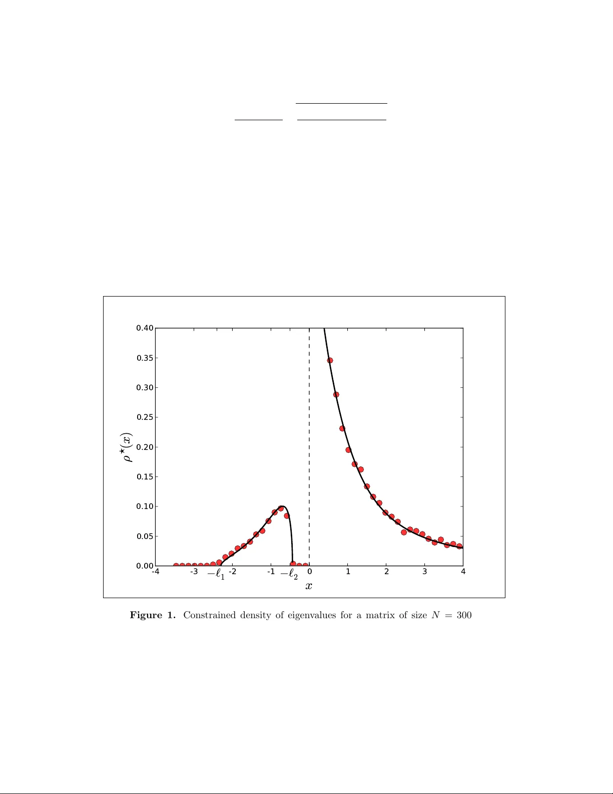
Index Distribution of Cauc h y Random Matrices Ricardo Marino, Sat ya N. Ma jumdar, Gr ´ egory Sc hehr and Pierpaolo Viv o Lab oratoire de Ph ysique Th ´ eorique et Mo d ` eles Statistiques, UMR 8626, Univ ersit ´ e P aris Sud 11 and CNRS, Bˆ at. 100, Orsa y F-91405, F rance Abstract. Using a Coulom b gas tec hnique, w e compute analytically the probabilit y P ( C ) β ( N + , N ) that a large N × N Cauc h y random matrix has N + p ositiv e eigen v alues, where N + is called the index of the ensem ble. W e show that this probability scales for large N as P ( C ) β ( N + , N ) ≈ exp − β N 2 ψ C ( N + / N ) , where β is the Dyson index of the ensem ble. The rate function ψ C ( κ ) is computed in terms of single in tegrals that are easily ev aluated numerically and amenable to an asymptotic analysis. W e find that the rate function, around its minimum at κ = 1 / 2, has a quadratic b ehavior modulated by a logarithmic singularity . As a consequence, the v ariance of the index scales for large N as V ar( N + ) ∼ σ C ln N , where σ C = 2 / ( β π 2 ) is t wice as large as the corresp onding prefactor in the Gaussian and Wishart cases. The analytical results are chec ked b y numerical simulations and against an exact finite N formula whic h, for β = 2, can b e deriv ed using orthogonal p olynomials. Index Distribution of Cauchy R andom Matric es 2 1. In tro duction Ensem bles of matrices with random en tries ha ve b een extensively studied since the seminal w orks of Wigner [ 1 ], Dyson [ 2 ] and Meh ta [ 3 ]. How ev er, many y ears b efore the official birth of Random Matrix Theory (RMT) in nuclear ph ysics in the 1950s, statisticians had already introduced some of the RMT machinery in their studies on multiv ariate analysis [ 4 , 5 , 6 ]. Restricting our scop e to matrices with real sp ectra, tw o main classes of ensem bles are typically considered, ι ) matrices with indep enden t en tries, and ιι ) matrices with rotational inv ariance. While limited analytical insigh t is generally av ailable for the former, rotationally inv ariant ensembles of N × N matrices are generally c haracterized b y a joint probability density function (jp df ) of the N real eigenv alues of the form P β ( λ ) = 1 Z N ,β Y j 0 , . . . , λ N > 0] = Prob[ λ min > 0], i.e. the probability that the smallest eigen v alue λ min is p ositiv e. Hence there is a natural connection betw een the index problem and the distribution of extreme eigenv alues, tackled in [ 8 , 9 , 13 , 43 , 44 ]. Note that the index problem in the complex plane (i.e. the s tatistics of the num b er of complex eigenv alues with mo dulus greater than a threshold) has also b een recently considered [ 45 , 46 ]. Expanding the rate function ψ G ( κ ) around the minim um, it w as found that it do es not displa y a simple quadratic b ehavior as one could ha ve naively exp ected. Instead, the quadratic b ehavior is mo dulated b y a logarithmic singularity , implying that in the close vicinity of N + = N / 2 ov er a scale of √ ln N one recov ers a Gaussian distribution, P ( G ) β ( N + , N ) ≈ exp " − ( N + − N / 2) 2 2 (V ar( N + )) # for N + → N / 2 , (5) with V ar( N + ) ∼ σ G ln N + C β + O (1 / N ) , σ G = 1 β π 2 . (6) Note that for β = 1 one recov ers the result in [ 36 ]. The constant term C 2 w as found [ 42 ] via the asymptotic expansion of a finite- N v ariance form ula conjectured by Prellb erg and later rigorously established [ 47 ]. In terestingly , the same analysis p erformed on p ositive definite Wishart matrices [ 48 ] for a threshold at ζ within the supp ort of the sp ectral density leads to V ar( N + ( ζ )) ∼ σ G ln N + O (1) , (7) where the leading term is indep enden t of ζ and exactly identical to the Gaussian case. Note that an explicit form ula for the full probabilit y of the index for finite N is not a v ailable to date in either case. Giv en the rather robust large N b eha vior of the v ariance which holds b oth for Gaussian matrices ( 6 ) and Wishart matrices ( 7 ), we inv estigate here the index probability distribution of § Hereafter, ≈ stands for a logarithmic equiv alence, lim N →∞ − ln P ( G ) β ( N + = κN ,N ) β N 2 = ψ G ( κ ). Index Distribution of Cauchy R andom Matric es 5 y et another ensemble of random matrices for which we exp ect a different b ehavior. W e consider indeed the Cauc hy ensem ble of N × N matrices H which are real symmetric ( β = 1), complex Hermitian ( β = 2) or quaternion self-dual ( β = 4). The Cauch y ensemble is characterized by the follo wing probability measure P ( H ) ∝ det 1 N + H 2 − β ( N − 1) / 2 − 1 , (8) where 1 N is the iden tity matrix N × N . The definition ( 8 ) is evidently in v arian t under the similarit y transformation H → UHU − 1 , where U is an orthogonal ( β = 1), unitary ( β = 2) or symplectic ( β = 4) matrix. The jp df of the N real eigenv alues can b e then immediately written as P β ( λ ) ∝ N Y j =1 1 (1 + λ 2 j ) β ( N − 1) / 2+1 Y ij ln | λ i − λ j | . (18) In this form, the jp df ( 17 ) mimics the Gibbs-Boltzmann w eight of a system of charged particles in equilibrium under competing in teractions. F ollowing Dyson [ 2 ] w e can treat this system for large N as a con tinuous fluid, described by a normalized densit y ρ ( λ ) = (1 / N ) P N i =1 δ ( λ − λ i ). Consequen tly , the m ultiple in tegral in ( 16 ) can b e conv erted in to a functional in tegral in the space of normalizable densities. This pro cedure w as first successfully employ ed to compute the large deviation of maximal eigenv alue of Gaussian matrices [ 43 ] and afterwards applied in sev eral differen t contexts [ 7 , 8 , 9 , 13 , 42 ]. In the contin uum limit, the multiple in tegral ( 16 ) b ecomes P ( C ) β ( N + ( ζ ) , N ) ∝ Z D [ ρ ] Z dA 1 Z dA 2 e − β 2 N 2 S [ ρ ] , (19) where the action S is given by S [ ρ ] = Z + ∞ - ∞ dxρ ( x ) ln(1 + x 2 ) − Z Z + ∞ - ∞ dxdx 0 ρ ( x ) ρ ( x 0 ) ln | x − x 0 | (20) + A 1 Z + ∞ - ∞ dxρ ( x ) − 1 + A 2 Z + ∞ ζ dxρ ( x ) − κ , (21) and A 1 , A 2 are Lagrange m ultipliers, introduced to enforce the o verall normalization of the densit y , and a fraction κ of eigenv alues exceeding ζ . The action S has an evident ph ysical meaning: it represen ts the free energy of the Coulomb fluid, whose particles are constrained to split ov er tw o regions of the real line, a fraction κ to the right of ζ and a fraction 1 − κ to the left of ζ . This Index Distribution of Cauchy R andom Matric es 8 free energy scales as N 2 (and not just N ) b ecause of the strong all-to-all in teractions among the particles. The energetic comp onent ∼ O ( N 2 ) of this free energy dominates o ver the entropic part ∼ O ( N ), making it p ossible to use a saddle p oin t metho d (see b elow). Note that the en tropic term has b een thoroughly studied and emplo y ed to define in terp olating ensem bles in [ 60 , 61 ]. As men tioned earlier, the integral ( 19 ), where w e neglected terms of O ( N ), can b e ev aluated using a saddle point metho d for large N . The c onstr aine d density of eigen v alues ρ ? ( x ) (dep ending parametrically on κ and ζ ) is determined b y the following v ariational condition δ S δ ρ = ln(1 + x 2 ) − 2 Z + ∞ −∞ dx 0 ρ ? ( x 0 ) ln | x − x 0 | + A 1 + A 2 θ ( x − ζ ) = 0 . (22) This Eq. ( 22 ), v alid for x inside the supp ort of ρ ? ( x ), can b e differentiated once with resp ect to x to give the follo wing singular integral equation x 1 + x 2 + A 2 δ ( x − ζ ) = P Z ∞ −∞ ρ ? ( y ) x − y dy , (23) where P stands for Cauch y principal part. Solving ( 23 ) with the constrain t R ∞ ζ dxρ ? ( x ) = κ is the main technical challenge. The physical intuition, supp orted by numerical simulations, p oints to wards a densit y supp orted on tw o disconnected interv als (see Fig. 1 ): for κ > 1 / 2, a compact blob with tw o edges to the left of ζ , and a non-compact blob to the right of ζ , extending all the w ay to infinity and with a singularit y for x → ζ + (for κ < 1 / 2 the situation is reversed, while only for κ = 1 / 2 the tw o blobs merge into the unconstrained single-supp ort densit y ρ ? C ( λ ) ( 11 )). In suc h a situation, the standard in v ersion formula [ 62 ] for singular integral equation of the type in ( 23 ) cannot b e applied, as it holds only for single supp ort (“one-cut”) solutions. How ev er, a more general metho d, whic h we no w present, allo ws to compute the r esolvent (or Green’s function) for this tw o-cuts problem k , and from it to deduce ρ ? . W e introduce the r esolvent G ( z ) = Z ρ ? ( x ) z − x dx , (24) for the Cauc hy case. It is an analytic function in the complex plane outside the supp ort of the densit y . F rom the resolven t, the density can b e computed in the standard wa y as 1 π lim ε → 0 Im G ( x + i ε ) = ρ ? ( x ) , (25) where Im stands for the imaginary part. Unc onstr aine d c ase. As a w arm-up exercise, we first deriv e the resolven t equation (using purely algebraic manipulations) for the unc onstr aine d case (corresp onding to ( 23 ) when A 2 = 0), where we exp ect to recov er the density ρ ? C ( x ) in Eq. ( 11 ). First, we multiply b oth sides in ( 23 ) (dropping the principal v alue) by ρ ? ( x ) / ( z − x ) and we in tegrate it ov er x , obtaining Z x 1 + x 2 ρ ? ( x ) z − x dx = Z Z ρ ? ( x ) ρ ? ( y ) ( x − y )( z − x ) dxdy . (26) k See [ 63 ] for a more sophisticated approach based on loop equation techniques. Index Distribution of Cauchy R andom Matric es 9 Our goal is to express b oth sides in terms of G ( z ) and, by doing so, obtain an algebraic equation for G ( z ). W e start b y the right hand side (RHS) where we use the simple identit y 1 ( z − x )( x − y ) = 1 z − x + 1 x − y 1 z − y . (27) Hence the RHS of ( 26 ) can b e written as Z Z ρ ? ( x ) ρ ? ( y ) ( x − y )( z − x ) dxdy = Z Z 1 z − x + 1 x − y ρ ? ( x ) ρ ? ( y ) z − y dxdy = Z Z ρ ? ( x ) ρ ? ( y ) ( z − x )( z − y ) dxdy + Z Z ρ ? ( x ) ρ ? ( y ) ( x − y )( z − y ) dxdy . (28) The second term of the sum in ( 28 ) (under the replacemen t x ↔ y ) is the original RHS of ( 26 ) with the sign c hanged. The first term of the sum is just G ( z ) 2 . Hence, w e hav e that the RHS of ( 26 ) is just equal to (1 / 2) G ( z ) 2 : Z Z ρ ? ( x ) ρ ? ( y ) ( x − y )( z − x ) dxdy = 1 2 G ( z ) 2 . (29) The left hand side (LHS) of ( 26 ) requires a little more algebraic manipulation to b e expressed in terms of G ( z ). W e manipulate this expression in t wo differen t w ays and exploit the equality b etw een the results to get rid of one in tegral. First, using the iden tit y x/ (1 + x 2 ) = 1 /x − 1 / ( x (1 + x 2 )) one has Z x 1 + x 2 ρ ? ( x ) z − x dx = Z 1 x ρ ? ( x ) z − x dx − Z 1 x (1 + x 2 ) ρ ? ( x ) z − x dx . (30) Note that in this splitting the tw o integrals in the RHS are individually div ergen t due to the p ole at x = 0, but the divergence cancels out b et ween the t wo. W e ma y regularize eac h individually div ergent in tegral by adding a small imaginary part in the denominator that is remov ed at the end of the calculation. Using the relation ( 27 ), we ma y express the first term of the sum in ( 30 ) as Z 1 x ρ ? ( x ) z − x dx = Z 1 x + 1 z − x ρ ? ( x ) z dx = 1 z Z ρ ? ( x ) x dx | {z } a 0 + 1 z Z ρ ? ( x ) z − x dx | {z } G ( z ) = a 0 z + G ( z ) z . (31) The second term of the sum in ( 30 ) will not b e calculated for now, and will b e called − α ( z ). Using this manipulation ( 31 ), we ha ve: Z x 1 + x 2 ρ ? ( x ) z − x dx = a 0 z + G ( z ) z − α ( z ) . (32) Index Distribution of Cauchy R andom Matric es 10 No w, w e use a different strategy , using the identit y x/ (1 + x 2 ) = ( x − z ) / (1 + x 2 ) + z / (1 + x 2 ), to obtain Z x 1 + x 2 ρ ? ( x ) z − x dx = Z x + z − z 1 + x 2 ρ ? ( x ) z − x dx = − Z ρ ? ( x ) 1 + x 2 dx | {z } a 1 + z Z 1 1 + x 2 ρ ? ( x ) z − x dx. (33) The first term in the sum ( 33 ) is a constan t, whic h w e call a 1 . No w w e pro ceed to manipulate the second term in ( 33 ) to obtain z Z 1 1 + x 2 ρ ? ( x ) z − x dx = z Z x − z + z x (1 + x 2 ) ρ ? ( x ) z − x dx (34) = − z Z ρ ? ( x ) x (1 + x 2 ) dx | {z } a 2 + z 2 Z 1 x (1 + x 2 ) ρ ? ( x ) z − x dx | {z } α ( z ) . (35) Therefore, the LHS of ( 26 ) can also b e written as − a 1 − z a 2 + z 2 α ( z ). W e ha ve then t wo distinct wa ys of writing the LHS, and we can use them b oth to cancel α ( z ): a 0 z + G ( z ) z − α ( z ) = (RHS) = − a 1 − z a 2 + z 2 α ( z ) . (36) Eliminating α ( z ) and recalling that the RHS is equal to (1 / 2) G ( z ) 2 ( 29 ), we find the algebraic equation for G ( z ) − a 1 + z ( a 0 − a 2 ) + z G ( z ) = (1 + z 2 ) 2 G ( z ) 2 . (37) W e pro ceed to determine the constants a 0 , a 1 and a 2 using the normalization condition of the density ρ ? ( x ). F rom ( 24 ) (setting | z | → ∞ ), it implies that G ( z ) should asymptotically go as G ( z ) ∼ 1 /z . T aking the limit | z | → ∞ in equation ( 37 ), we find equations for the co efficients − a 1 + z ( a 0 − a 2 ) + z 1 z + O ( z − 2 ) = z 2 2 1 z + O ( z − 2 ) 2 , (38) whic h implies a 0 = a 2 and a 1 = 1 2 . Our algebraic equation, finally , b ecomes: (1 + z 2 ) G ( z ) 2 − 2 z G ( z ) + 1 = 0 . (39) The tw o solutions read G ( z ) = 2 z ± p 4 z 2 − 4(1 + z 2 ) 2(1 + z 2 ) = z ± i 1 + z 2 . (40) Using ( 25 ), the densit y comes out as exp ected 1 π lim ε → 0 Im G ( x + i ε ) = 1 π 1 1 + x 2 = ρ ? C ( x ) . (41) Index Distribution of Cauchy R andom Matric es 11 Constr aine d c ase. Now, w e consider the full index problem, i.e. with an extra term in the p oten tial as in ( 23 ), x 1 + x 2 + A 2 δ ( x − ζ ) = P Z ∞ −∞ ρ ? ( y ) x − y dy , (42) where the constant A 2 will b e determined b y the new normalization condition of the rightmost blob R ∞ ζ ρ ? ( x ) dx = κ . W e rep eat the same steps as for the unconstrained in tegral equation, m ultiplying ( 23 ) (without the principal v alue) by ρ ? ( x ) z − x and in tegrating ov er x . W e get an extra term compared to Eq. ( 26 ), arising from the Lagrange multiplier Z x 1 + x 2 ρ ? ( x ) z − x dx = Z Z ρ ? ( x ) ρ ? ( y ) ( x − y )( z − y ) dxdy − A 2 z − ζ . (43) W e absorb this new term in to the RHS and proceed to express, as b efore, all integrals in terms of G ( z ). Our new algebraic equation will then b e: − a 1 + z ( a 0 − a 2 ) + z G ( z ) = (1 + z 2 ) G ( z ) 2 2 − A 2 z − ζ . (44) Imp osing the condition that G ( z ) ∼ 1 /z for | z | → ∞ , we get the tw o conditions a 1 = 1 / 2 and a 0 − a 2 + A 2 = 0. Calling A 2 = B / 2, for ζ = 0 we get the equation B 2 z + G ( z ) z − 1 2 = z 2 + 1 B / 2 z + G ( z ) 2 2 , (45) whose solutions are G ( z ) = z 2 ± √ − B z 3 − B z − z 2 z 3 + z . (46) Using ( 25 ), it is then easy to derive that the constrained density is: ρ ? ( x ) = 1 π p B ( x 3 + x ) + x 2 | x 3 + x | , (47) or equiv alently ρ ? ( x ) = 1 π (1 + x 2 ) r B ( x + ` 1 )( x + ` 2 ) x , (48) where the edge p oin ts of the leftmost blob (for κ > 1 / 2) − ` 1 , − ` 2 are determined as a function of B ` 1 = 1 2 B (1 + √ 1 − 4 B 2 ) , (49) ` 2 = 1 2 B (1 − √ 1 − 4 B 2 ) . (50) Index Distribution of Cauchy R andom Matric es 12 The functional form in Eq. ( 48 ) holds for x b elonging to any of the tw o supp orts. The constan t B is then determined as a function of κ by Z ∞ 0 dx 1 π (1 + x 2 ) r B ( x + ` 1 )( x + ` 2 ) x = κ . (51) F or κ → 1 / 2 (unconstrained case), the solution is B → 0, and ρ ? ( x ) → ρ ? C ( x ) as exp ected. This means that we recov er the unconstrained Cauch y case if we imp ose a num b er of p ositive eigen v alues exactly equal to N / 2, and this unconstrained case materializes when B → 0. As κ approac hes 1 / 2, the ` 2 edge mo ves tow ards the origin, while the other edge ` 1 approac hes infinity , un til exactly at the critical p oint κ = 1 / 2 the tw o blobs merge back together. In Fig. 1 , we sho w a plot of the density ( 48 ) for κ = 0 . 9. W e also show standard Mon te Carlo simulations of N = 300 particles distributed according to the Boltzmann w eight ∝ e − β H [ λ ] under the Hamiltonian H [ λ ] in ( 18 ), with the constrain t that 90% of them are forced to sta y on the p ositive semi axis . W e observ e a nice agreemen t b et ween our exact form ula and the numerics. -4 -3 -2 -1 0 1 2 3 4 − ` 1 − ` 2 x 0.00 0.05 0.10 0.15 0.20 0.25 0.30 0.35 0.40 ρ ( x ) Figure 1. Constrained density of eigenv alues for a matrix of size N = 300 where 90% of the eigen v alues are forced to lie on the p ositiv e semi axis and the corresponding exp ected theoretical curv e for κ = 0 . 9 [ B = 0 . 36613 ... from ( 51 )]. Finally , from ( 19 ), w e obtain the decay of the probability of the index for large N as P ( C ) β ( N + , N ) ≈ exp − β N 2 ψ C ( N + / N ) , (52) Index Distribution of Cauchy R andom Matric es 13 with ψ C ( κ ) = 1 2 S [ ρ ? ] − S [ ρ ? ] κ =1 / 2 , (53) where the additional term S [ ρ ? ] κ =1 / 2 comes from normalization. In the next section, we simplify the action ( 21 ) at the saddle p oint and express it in terms of t wo single in tegrals which are hard to ev aluate in closed form. The resulting rate function ( 53 ) can anyw ay b e efficiently ev aluated numerically with arbitrary precision. 3. Computation of the rate function The action ( 21 ) ev aluated at the saddle p oint densit y ( 48 ) reads S [ ρ ? ] = Z + ∞ - ∞ dxρ ? ( x ) ln(1 + x 2 ) − Z Z + ∞ - ∞ dxdx 0 ρ ? ( x ) ρ ? ( x 0 ) ln | x − x 0 | + A 1 Z + ∞ - ∞ dxρ ? ( x ) − 1 + A 2 Z + ∞ 0 dxρ ? ( x ) − κ . (54) Since by construction ρ ? ( x ) satisfies the normalization conditions, the terms in the second line are automatically zero. W e can no w replace the double integral with single in tegrals. W e use equation ( 22 ) for ζ = 0, 2 Z + ∞ −∞ dx 0 ρ ? ( x 0 ) ln | x − x 0 | = ln(1 + x 2 ) + A 1 + A 2 θ ( x ) . (55) Multiplying this expression by ρ ? ( x ) and integrating o v er x we obtain Z Z + ∞ - ∞ dxdx 0 ρ ? ( x ) ρ ? ( x 0 ) ln | x − x 0 | = 1 2 Z + ∞ - ∞ dxρ ? ( x ) ln(1 + x 2 ) + A 1 + A 2 κ . (56) Inserting ( 56 ) in ( 54 ) we obtain S [ ρ ? ] = 1 2 Z + ∞ - ∞ dxρ ? ( x ) ln(1 + x 2 ) − A 1 2 − A 2 2 κ. (57) W e must no w determine the constan ts A 1 and A 2 . T o do so, w e first consider, without loss of generality , the case κ > 1 2 , where the densit y has the shap e as in Fig. 1 . The left blob has a compact supp ort [ − ` 1 , − ` 2 ]. T o determine the relation b etw een A 1 and A 2 , we study the asymptotic b ehavior of equation ( 55 ) when x → + ∞ . Since b oth 2 R + ∞ −∞ dx 0 ρ ? ( x 0 ) ln | x − x 0 | and ln(1 + x 2 ) b ehav e like 2 ln( x ) in the large x limit, w e deduce that A 1 = − A 2 . Ev aluating ( 55 ) at x = − ` 1 , we find the v alue of A 1 , and hence A 2 , in terms of ` 1 : A 1 = 2 Z + ∞ - ∞ dxρ ? ( x ) ln | x + ` 1 | − ln(1 + ` 2 1 ) . (58) Index Distribution of Cauchy R andom Matric es 14 W e may finally write the action at the saddle p oint as S [ ρ ? ] = 1 2 Z + ∞ - ∞ dxρ ? ( x ) ln(1 + x 2 ) | {z } I 1 − (1 − κ ) Z + ∞ - ∞ dxρ ? ( x ) ln | x + ` 1 | | {z } I 2 + (1 − κ ) 2 ln(1 + ` 2 1 ) | {z } I 3 . (59) where ρ ? ( x ) (dep ending parametrically on κ ) is given in Eq. ( 48 ). The single integrals I 1 and I 2 do not seem expressible in closed form. Ho wev er the rate function ( 53 ) can b e plotted without difficult y (see Fig. 2 ). One can see that the rate function is symmetric, has a minim um at κ = 1 / 2, corresp onding to the “typical” situation, where half of the eigen v alues are p ositiv e and half are negativ e. In the extreme limit κ = 0 (which is the same as κ = 1), we get ψ C ( κ = 0) = 1 2 S [ ρ ? ] κ =0 − S [ ρ ? ] κ =1 / 2 = ln 2 4 ≈ 0 . 173287 ... (60) in agreement with the large deviation law for the largest Cauch y eigenv alue [Eq. (13) in [ 56 ] for w = 0]. 0.0 0.2 0.4 0.6 0.8 1.0 κ 0.00 0.02 0.04 0.06 0.08 0.10 0.12 0.14 0.16 0.18 ψ C ( κ ) Figure 2. Plot of the rate function ψ C ( κ ). In the next section, w e p erform a careful asymptotic analysis of the rate function ψ C ( κ ) around the minim um κ = 1 / 2, whic h brings a quadratic b eha vior mo dulated by a logarithmic singularit y . This is in turn resp onsible for the logarithmic growth of the v ariance of the index with N (to leading order), and pro vides the correct prefactor. Index Distribution of Cauchy R andom Matric es 15 4. Asymptotic analysis of ψ C ( κ ) in the vicinit y of κ = 1 / 2 W e ha ve already remark ed that the typical situation κ = 1 / 2 is realized when the constan t B → 0. Therefore it is necessary to expand the terms I 1 , I 2 and I 3 in the action ( 59 ), as well as the in tegral constraint ( 51 ), for B → 0. It turns out that this calculation is highly nontrivial, as several cancellations o ccur in the leading and next-to-leading terms of each con tribution (see App endix A for details). Denoting κ = 1 / 2 + δ (with δ → 0), the final result reads: S [ ρ ? ] ∼ ln 2 + π 2 B δ + o ( δ ) . (61) In App endix A , we sho w that the relation b etw een δ and B is (to leading order for δ → 0) δ ∼ − B ln | B | π . (62) In verting this relation, w e find to leading order B ∼ − π δ ln | δ | , (63) implying from ( 61 ) that S [ ρ ? ] ∼ ln 2 − π 2 2 δ 2 ln | δ | + o ( δ ) . (64) Therefore ψ ( κ = 1 / 2 + δ ) = S [ ρ ? ] − S [ ρ ? ] κ =1 / 2 ∼ − π 2 2 δ 2 ln | δ | for δ → 0 . (65) F rom ( 52 ), w e then hav e (for N + close to N / 2) P ( C ) β N + = 1 2 + δ N , N ≈ exp β N 2 2 π 2 δ 2 2 ln | δ | . (66) Restoring δ = ( N + − N / 2) / N in the RHS of ( 66 ), we obtain the Gaussian b eha vior announced in the introduction [Eq. ( 14 )]: P ( C ) β ( N + , N ) ≈ exp − ( N + − N / 2) 2 2 (V ar( N + )) ! for N + → N / 2 , (67) with V ar( N + ) ∼ 2 β π 2 ln N + O (1) . (68) In the next section, w e compare the asymptotic b ehavior of the v ariance with a closed expression v alid for finite N and β = 2, finding p erfect agreement b et w een the trends. Index Distribution of Cauchy R andom Matric es 16 5. Exact deriv ation for the v ariance of N + for finite N and β = 2 In App endix B , we derive a general form ula for the v ariance of any linear statistics at finite N and β = 2. Sp ecializing it to the index case, we deduce that V ar( N + ) = N 2 − Z Z ∞ 0 dλdλ 0 [ K N ( λ, λ 0 )] 2 , (69) where K N ( λ, λ 0 ) is the kernel of the ensemble, built up on suitable orthogonal p olynomials. It turns out that in the Cauc hy case, the orthogonal p olynomials π n ( x ) satisfying Z ∞ −∞ dx π n ( x ) π m ( x ) (1 + x 2 ) N = δ mn (70) are π n ( x ) = i n 2 N n !( N − n − 1 2 )Γ 2 ( N − n ) 2 π Γ(2 N − n ) 1 / 2 P ( − N , − N ) n (i x ) , (71) where P ( − N , − N ) n ( x ) are Jacobi p olynomials. The kernel then reads K N ( λ, λ 0 ) = 1 (1 + λ 2 ) N/ 2 1 (1 + λ 0 2 ) N/ 2 N − 1 X j =0 π j ( λ ) π j ( λ 0 ) , (72) and inserting ( 72 ) in to ( 69 ) we obtain after simple algebra V ar( N + ) = N 4 − 2 N − 1 X n 1 / 2) ρ ? ( x ) is [ − ` 1 , − ` 2 ] ∪ (0 , + ∞ ), therefore we need to consider the tw o blobs of each term in the action separately . • I 1 = 1 2 R ∞ −∞ dxρ ? ( x ) ln(1 + x 2 ) . First, we separate the in tegral as I 1 = I L 1 + I R 1 I L 1 = 1 2 Z − ` 2 − ` 1 dxρ ? ( x ) ln(1 + x 2 ) , I R 1 = 1 2 Z + ∞ 0 dxρ ? ( x ) ln(1 + x 2 ) . (A.1) Index Distribution of Cauchy R andom Matric es 21 W riting I R 1 explicitly we obtain I R 1 = 1 2 π Z + ∞ 0 dx p B ( x 3 + x ) + x 2 x ( x 2 + 1) ln(1 + x 2 ) . (A.2) T o compute the asymptotic b ehavior when B → 0, w e split this in tegral in to tw o parts, one in tegral from 0 to B and one from B to ∞ : I R 1 = 1 2 π Z B 0 dx p B ( x 3 + x ) + x 2 x ( x 2 + 1) ln(1 + x 2 ) + Z ∞ B dx p B ( x 3 + x ) + x 2 x ( x 2 + 1) ln(1 + x 2 ) ! . (A.3) No w w e can expand the in tegrands in series around B = 0 and in tegrate term by term to obtain [up to order O ( B )] I R 1 − − − → B → 0 ln 2 2 + B ln 2 ( B ) 4 π − B ln( B ) 2 π (1 + ln 4) + B 4 π 2 + 4 ln 2(1 + ln 2) + 3 π 2 4 + o ( B ) . (A.4) W e now turn our attention to I L 1 , calculating the asymptotic b ehavior when B → 0 of the in tegral: I L 1 = 1 2 π Z − ` 2 − ` 1 dx p B ( x 3 + x ) + x 2 | x ( x 2 + 1) | ln(1 + x 2 ) . (A.5) T o pro ceed, it is more conv enient to reexpress I L 1 in terms of its edge p oints I L 1 = √ B 2 π Z − ` 2 − ` 1 dx p − ( x + ` 1 )( x + ` 2 ) p | x | ( x 2 + 1) ln(1 + x 2 ) , (A.6) whic h is equiv alen t to ( A.5 ). W e pro ceed with the follo wing change of v ariable y = x + ` 1 ` 1 − ` 2 , we ha ve: I L 1 = √ B 2 π Z 1 0 ( ` 1 − ` 2 ) dy 1 + [( ` 1 − ` 2 ) y − ` 1 ] 2 ( ` 1 − ` 2 ) p y (1 − y ) p | ( ` 1 − ` 2 ) y − ` 1 | ln 1 + [( ` 1 − ` 2 ) y − ` 1 ] 2 . (A.7) Since ` 1 b eha v es lik e 1 B − B and ` 2 b eha v es lik e B when B is small, ` 1 − ` 2 go es as 1 B − 2 B . W e replace these asymptotic behaviors in ( A.7 ), k eeping only the leading orders for small B . The resulting in tegral can b e computed explicitly and w e can then extract its asymptotic b ehavior when B → 0 I L 1 − − − → B → 0 ln 2 2 − B ln 2 B 4 π + (1 + ln 4)( B ln B ) 2 π + B 4 π π 2 4 − 2 − 4 ln 2(1 + ln 2) + o ( B ) (A.8) Note an impressive series of cancellations in the sum I L 1 + I R 1 , resulting in I 1 − − − → B → 0 ln 2 + π 4 B + o ( B ) . (A.9) Index Distribution of Cauchy R andom Matric es 22 • I 2 = R ∞ −∞ dxρ ? ( x ) ln( ` 1 + x ). First, we again separate the integral ov er the tw o supp orts I 2 = I L 2 + I R 2 I L 2 = Z − ` 2 − ` 1 dxρ ? ( x ) ln( ` 1 + x ) I R 2 = Z + ∞ 0 dxρ ? ( x ) ln( ` 1 + x ) . (A.10) Both integrals are very similar to I R 1 and I L R , and w e pro ceed to calculate them b y the same metho ds. Expanding the integrals to leading orders of B and adding b oth terms, we get to I 2 − − − → B → 0 − ln B + π 2 B + o ( B ) . (A.11) The third term, I 3 , has a straightforw ard expansion I 3 − − − → B → 0 − 2 ln B + o ( B ) . (A.12) The action S [ ρ ? ] at the saddle p oint has therefore an expansion for B → 0 equal to S [ ρ ? ] ∼ ln 2 + π 4 B − (1 − κ ) − ln B + π 2 B + (1 − κ ) 2 ( − 2 ln B ) + o ( B ) . (A.13) Once we write κ = 1 2 + δ , we obtain Eq. ( 61 ). App endix B. General form ula for the v ariance of a linear statistics at finite N for β = 2 W e derive here a general fluctuation formula (v alid for β = 2 and finite N ) for the v ariance of a line ar statistics , i.e. a random v ariable φ of the form φ = N X i =1 f ( λ i ) , (B.1) for a general b enign function f ( x ). The v ariance of φ is giv en b y V ar( φ ) = h φ 2 i − h φ i 2 , where the a verage is tak en with resp ect to the jp d of the N eigen v alues P ( λ 1 , . . . , λ N ). By definition h φ 2 i = Z · · · Z dλ 1 . . . dλ N P ( λ 1 , . . . , λ N ) N X i =1 f ( λ i ) N X j =1 f ( λ j ) . (B.2) Let us first define the one-p oin t and the t wo-point correlation function (marginals) of the jpdf P ( λ 1 , . . . , λ N ) ¶ R 1 ( λ ) = N Z · · · Z dλ 2 . . . dλ N P ( λ, λ 2 , . . . , λ N ) , (B.3) R 2 ( λ, λ 0 ) = N ( N − 1) Z · · · Z dλ 3 . . . dλ N P ( λ, λ 0 , λ 3 , . . . , λ N ) . (B.4) ¶ The one-p oint function R 1 ( λ ) is related to the finite- N sp ectral density via R 1 ( λ ) = N ρ N ( λ ). Index Distribution of Cauchy R andom Matric es 23 Separating in the double sum in ( B.2 ) the term i = j from the terms i 6 = j w e easily obtain h φ 2 i = Z dλR 1 ( λ ) [ f ( λ )] 2 + Z Z dλdλ 0 f ( λ ) f ( λ 0 ) R 2 ( λ, λ 0 ) , (B.5) while clearly h φ i 2 = Z dλR 1 ( λ ) f ( λ ) 2 . (B.6) The theory of orthogonal p olynomials [ 64 ] gives a prescription to compute n -p oin t correlation functions for β = 2 in terms of a n × n determinant. More precisely , let P ( λ 1 , . . . , λ N ) ∝ Y j
Original Paper
Loading high-quality paper...
Comments & Academic Discussion
Loading comments...
Leave a Comment