Self-similar prior and wavelet bases for hidden incompressible turbulent motion

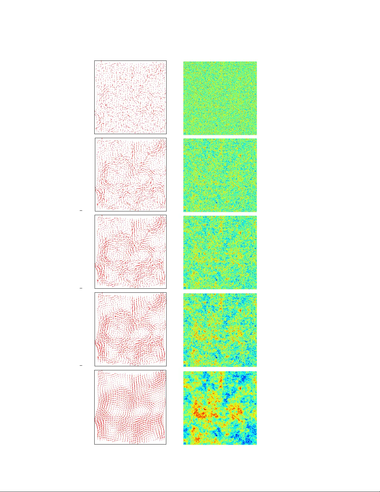
SELF-SIMILAR PRIOR AND W A VELET BASES F OR HIDDEN INCOMPRESSIBLE TURBULENT MOTION P . H ´ EAS ∗ , F. LA V ANCIER † , AND S. KADRI-HAR OUNA ‡ Abstract. This work is concerned with the ill-posed inv erse problem of estimating turbulent ﬂows from the observ ation of an image sequence. F rom a Ba y esian p erspective, a divergence-free isotropic fractional Brownian motion (fBm) is chosen as a prior model for instantaneous turbulent velocity ﬁelds. This self-similar prior characterizes accurately second-order statistics of velocity ﬁelds in incompressible isotropic turbulence. Nevertheless, the associated maximum a p osteriori inv olves a fractional Laplacian operator whic h is delicate to implement in practice. T o deal with this issue, w e propose to decompose the div ergence-free fBm on w ell-chosen wa v elet bases. As a ﬁrst alternative, w e prop ose to design wa velets as whitening ﬁlters. W e show that these ﬁlters are fractional Laplacian wa velets comp osed with the Lera y pro jector. As a second alternativ e, we use a divergence-free w a v elet basis, which tak es implicitly into accoun t the incompressibilit y constraint arising from ph ysics. Although the latter decomposition inv olv es correlated w av elet coeﬃcients, w e are able to handle this dep endence in practice. Based on these t w o wa v elet decomp ositions, we ﬁnally provide eﬀectiv e and eﬃcient algorithms to approach the maximum a p osteriori. An intensiv e numerical evaluation proves the relev ance of the prop osed wa v elet-based self-similar priors. Key w ords. Bay esian estimation, fractional Brownian motion, divergence-free wa velets, frac- tional Laplacian, connection co eﬃcien ts, fast transforms, optic-ﬂo w, isotropic turbulence. AMS sub ject classiﬁcations. 60G18, 60G22, 60H05, 62F15, 65T50, 65T60 1. In tro duction. This work is concerned with the ill-posed in v erse problem of estimating turbulen t motions from the observ ation of an image sequence. T urbulence motion phenomena are often studied in the con text of incompressible ﬂuids, which is the setting of this pap er. This inv erse problem arises in the con text of exp erimen tal ph ysical settings, where one is interested in recov ering the kinematical state of an incompressible turbulent ﬂuid ﬂow from the observ ation of a sequence of images, e.g. particle image v elocimetry in exp erimen tal ﬂuid mec hanics, wind or o cean currents retriev al from satellite imagery in geophysics. Solving accurately this type of inv erse problems constitute an imp ortant issue since a complete ph ysical theory is still missing for turbulence phenomenology . More sp eciﬁcally , the abov e inv erse problem can b e viewed as a Maxim um A P osteriori (MAP) estimation of a v ectorial ﬁeld u ov er a space of admissible solutions: u ∗ ( y 0 , y 1 ) ∈ arg max u p δ y | u p u , where y 0 and y 1 are t w o consecutiv e observed images, u is a v elo cit y ﬁeld, and δ y is a function of y 0 , y 1 and u , whic h characterizes the evolution b et w een y 0 and y 1 . In this problem, u is not observ ed and the incompressibilit y constrain t demands the motion ﬁeld u to be divergence-free. In this Ba yesian framework, p δ y | u denotes the lik eliho od model, whic h relates the motion of the physical system to the spatial and temp oral v ariations of the image intensit y . The adjunction of a prior information p u for the v elo cit y ﬁeld u is in this case mandatory since, as we will see in section 4, this non-linear problem is under-constrained. ∗ Inria Rennes, Centre de Bretagne A tlantique, Universit ´ e de Beaulieu, 35042 Rennes, F rance ( Patrick.Heas@inria.fr ) † Universit ´ e de Nan tes, Lab oratoire de Math´ ematiques Jean Leray , 2 rue de la Houssini` ere, 44322 Nantes, F rance ‡ Universit ´ e de La Ro c helle, 23 a ven ue Alb ert Einstein, 17071 La Ro chelle, F rance 1 2 Concerning the c hoice of p δ y | u , relev an t physical mo dels hav e b een prop osed for ﬂuid ﬂow imagery . A review in the context of exp erimen tal ﬂuid mechanics can b e found in [30]. W e will assume in this pap er the simple mo del where y 0 and y 1 are the solutions b etw een tw o consecutive times of a transport equation driven by u , see section 4 for more details. Concerning the c hoice of p u , the incompressible Na vier-Stok es equations perfectly describ e the structure of an incompressible velocity ﬁeld, i.e. the prior for u . Ho w ev er, this implicit choice of constraints leads to an optimization problem whic h is often sev erely ill-conditioned and computationally prohibitive. Some recent w orks prop ose to use a simpliﬁed v ersion of Navier-Stok es equations to circum v en t this issue (see e.g. [10, 38]). On the other hand, instead of relying the prior on the Navier-Stok es equations, spatial regularizers of u hav e b een proposed to serve as a prior. A ﬁrst approac h in this direction is to assume a lo w-dimensional parametric form for u , see e.g. [4, 13]. A s econd strategy is to choose a prior that in tro duces some spatial smo othness for u . Typically , the regularisation p enalises in this case the norm of the gradien t (or higher deriv ativ es) of u , see e.g. [24, 25, 45, 52]. Finally , a third approac h consists in the in tro duction of a self-similar constraint on u . Self-similarity is a well-kno wn feature of turbulence, theoretically and experimentally attested, see e.g. [36]. An attempt in this direction has been conducted in [21, 22]. Besides, a general family of self-similar regularizers has been introduced in [49]. In the same spirit, our choice for the prior of u is the divergence-free isotropic fractional Bro wnian motion (fBm), as we no w justify . In addition to self-similarity , w e assume u to b e Gaussian. Non-Gaussian tur- bulen t ﬁelds is an interesting alternativ e, which could potentially describe more ac- curately the structure of turbulence [18], but they will not been considered in this pap er. Note that the deﬁnition of such models is still an activ e domain of inv esti- gation, see [9, 27, 28, 36, 43]. Assuming further the stationarit y of the incremen ts of u leads necessarily to u being a v ector fBm (see [48]). In order to satisfy the incompressibilit y constraint, u is ﬁnally demanded to b e divergence-free. Although div ergence-free fBm’s can b e viewed as a limiting case of the vector fBm’s considered in [48], we pro vide a proper deﬁnition in section 2. In particular, a sp ectral in tegral represen tation is deduced. This choice of prior in volv es in practice fractional Laplacian operators, whic h are numerically delicate to implemen t. Indeed, there is a lac k of eﬀectiv e algorithms in the literature able to deal in practice with those particular priors. In [49], the authors circum v ent this issue in their numerical applications by limiting themselves to non-fractional settings. T o tackle this problem, we prop ose to decompose fBms on w ell-c hosen wa velet bases. This strategy allows us to expand fractional Laplacian op erators on the w a v elet components and mak es their computation feasible. W e fo cus on t w o particular w a v elet bases. - As a ﬁrst alternativ e, w e prop ose to design wa velets as whitening ﬁlters for div ergence-free isotropic fBms. F or scalar fBms indexed b y time, fractional w av elet bases represen t ideal whitening ﬁlters [16, 35]. In [46, 47, 48], the au- thors extend these bases to the case of isotropic v ector ﬁelds, namely they use the so-called fractional Laplacian p olyharmonic spline w a v elets. In our case of div ergence-free isotropic v ector fBms, we show that for any mother w av elet, fractional Laplacian wa v elet series composed with the Leray pro jector is an appropriate whitening ﬁlter. - The second alternativ e is to use div ergence-free w a v elet bases, which are w ell- Self-similar prior and wa velet bases for hidden incompressible turbulent motion 3 suited to our case. These wa velets simplify the decomp osition, since they do not in v olv e fractional op erators and make sup erﬂuous the use of Lera y pro- jector [14, 15, 26, 29]. Ho wev er, the w a v elets coeﬃcients are then correlated. As seen in section 5.1, implementation for the ﬁrst bases can b e accurately p erformed in the F ourier domain. F or the second bases, the computation of the asso ciated pos- terior density relies on the co v ariances of the wa v elet co eﬃcien ts. W e pro vide a closed form expression for these cov ariances, which allows us to prop ose an appro ximation of the posterior using wa velet connection co eﬃcients, see sections 5.2.1 and 5.2.2. Moreo ver, an additional pleasan t feature of wa v elet representations is that it is w ell adapted to the non-conv ex optimization problem of MAP estimation, since it naturally pro vides a multi-resolution approach. As a matter of fact, this approac h has pro v ed to b e experimentally eﬃcient for motion estimation problems (sub jected to diﬀeren t priors) [13, 25, 50]. The optimization algorithms rely on F ast F ourier T rans- forms (FFT) or on F ast W a v elet T ransforms (FWT). Finally , for the div ergence-free w av elet decomp osition, we introduce an appro ximated MAP optimization pro cedure, whic h turns out to be by far the fastest algorithm while being as accurate as the other approac hes. A n umerical comparison with state-of-the-art pro cedures is p erformed in section 6 on a general benchmark of div ergence-free fBm. Note that, while these ﬁelds match p erfectly our priors, they are lik ely to b e in agreemen t with real ﬂuid ﬂows according to turbulence phenomenology , as mentioned b efore. As a result, our pro cedure seems to recov er more accurately the hidden motion ﬁeld, in particular when the Hurst parameter H corresp onds to 2D and 3D turbulence mo dels, resp ectiv ely H = 1 and H = 1 3 according to ph ysics. The paper is organized as follows. In section 2, we give a spectral representation of divergence-free isotropic fBms, which will serve as the basic deﬁnition all along the pap er. In section 3, we then provide the tw o wa v elet representations described ab o v e. Section 4 displays the Bay esian mo deling of turbulent ﬂows in terms of w av elet co ef- ﬁcien ts and considers the asso ciated MAP estimators. In section 5, gradient descent optimization algorithms achieving MAP estimation are presented for b oth wa velet bases. The numerical ev aluation of the prop osed regularizers is presented in sec- tion 6. Finally , the app endix gathers the technical pro ofs and some details ab out the algorithms and the computation of fractional Laplacian wa v elet connection co ef- ﬁcien ts. 2. Sp ectral deﬁnition of div ergence-free isotropic fBm. The unique self- similar zero-mean Gaussian process with stationary increments is the fractional Bro w- nian motion (fBm), in tro duced in [34]. The deﬁnition of scalar fBm indexed by time has been extended: to the case of m ulti-dimensional state spaces, i.e. ve ctor processes indexed by time [2]; to the ﬁeld case, namely scalar isotr opic ﬁelds [41]; and to both cases, i.e. isotr opic ve ctor ﬁelds [36, 48]. As far as we are in terested in the construction of a prior for turbulent v ector ﬁelds, we are particularly concerned with diver genc e-fr e e isotropic v ector fBm in the follo wing sense. F or sak e of clarity , this work is restricted to the bi-v ariate case al- though it is p ossible to extend our results to higher dimensions. Definition 2.1. A bi-variate ﬁeld u ( x ) , ( u 1 ( x ) , u 2 ( x )) T , x ∈ R 2 , is a diver genc e-fr e e isotr opic bi-variate fBm with p ar ameter 0 < H < 1 if • u is Gaussian; • u is self-similar, i.e. for any λ > 0 , u ( λ x ) L = λ H u ( x ) ; 4 • u has stationary incr ements, i.e. ∀ h ∈ R 2 , u ( x ) − u ( x − h ) is stationary; • u is isotr opic, i.e. for any r otation matrix M , u ( x ) L = u ( M x ) ; • u is diver genc e-fr e e, i.e. div u = 0 almost sur ely. Since a fBm is almost surely not diﬀeren tiable, the divergence operator in the last prop ert y is to b e understoo d in a weak sense: for any test function ψ ∈ C 1 ( R 2 ) with a fast deca y at inﬁnity , div u , h div u , ψ i = −h u / ∇ ψ i , where h ., . i (resp. h ./. i ) denotes the inner pro duct of t w o scalar (resp. tw o bi-v ariate) functions, and ∇ denotes the gradient op erator. Let us remark that diﬀeren tiability in a w eak sense is a little bit sc hematic when compared to real ﬂo ws, since it is well kno wn that b elow the Kolmogoro v scale, the ﬁeld becomes smo oth. The fBm mo del only constitutes an appro ximation of turbulence, consistent with the range of scales mo delled in practice. Isotropic fractional Brownian v ector ﬁelds hav e b een introduced b y T afti and Unser [48] as the solution of a fractional Poisson equation, or whitening equation, see [47] and [48]. Isotropic diver genc e-fr e e fractional Bro wnian v ector ﬁelds, as we require, turns out to b e a limiting case of the solution (corresp onding to ξ irr = ∞ and ξ sol = 0 in the setting of [48]). Sp eciﬁcally , it can b e deﬁned b y: u = σ ( − ´ ∆) − H +1 2 div W , (2.1) where H ∈ (0 , 1) is the Hurst parameter, σ is a p ositiv e constan t, W is a vector of t w o indep enden t Gaussian white noise, and ( − ´ ∆) − H +1 2 div is a fractional Laplacian op erator, deﬁned for an y f in ( L 2 ( R 2 )) 2 b y ( − ´ ∆) − H +1 2 div f ( x ) = 1 (2 π ) 2 Z R 2 ( e i k · x − 1) k k k H +1  I − kk T k k k 2  F ( f )( k ) d k , where F ( f ) denotes the F ourier transform of f = ( f 1 , f 2 ) T in ( L 2 ( R 2 )) 2 , viz. F ( f )( k ) =  Z R 2 f 1 ( x ) e − i k · x d x , Z R 2 f 2 ( x ) e − i k · x d x  T . In the following proposition, we provide a spectral representation of u deﬁned b y (2.1). This prop osition gives an explicit representation, therefore it can also b e considered as an alternative deﬁnition. In fact, w e will only refer in the sequel to this represen tation when w e consider isotropic divergence-free fractional Brownian vector ﬁelds. Proposition 2.2. The isotr opic diver genc e-fr e e fr actional Br ownian ve ctor ﬁeld u , as deﬁne d by (2.1) admits the fol lowing r epr esentation, for any H ∈ (0 , 1) , u ( x ) = σ 2 π Z R 2 ( e i k · x − 1) k k k H +1  I − kk T k k k 2  ˜ W ( d k ) , x ∈ R 2 , (2.2) wher e I denotes the identity matrix and ˜ W = ( ˜ W 1 , ˜ W 2 ) T denotes a bi-variate stan- dar d Gaussian sp e ctr al me asur e, i.e. ˜ W 1 and ˜ W 2 ar e indep endent and for i = 1 , 2 , for any Bor el sets A, B in R 2 , ˜ W i ( A ) is a c enter e d c omplex Gaussian r andom variable, Self-similar prior and wa velet bases for hidden incompressible turbulent motion 5 ˜ W i ( A ) = ˜ W i ( − A ) and E ( ˜ W i ( A ) ˜ W i ( B )) = | A ∩ B | . As a by-product, we deduce the following structure matrix function that charac- terizes the law of the Gaussian vector ﬁeld u : for any i, j = 1 , 2, for any x 1 , x 2 , x 3 , x 4 in R 2 , Σ ij ( x 1 , x 2 , x 3 , x 4 ) , E [( u i ( x 2 ) − u i ( x 1 ))( u j ( x 4 ) − u j ( x 3 ))] = σ 2 c H  F H ij ( x 2 − x 3 ) − F H ij ( x 2 − x 4 ) − F H ij ( x 1 − x 3 ) + F H ij ( x 1 − x 4 )  , (2.3) where c H = Γ(1 − H ) / ( π 2 2 H +2 Γ( H + 1) H (2 H + 2)) with Γ( . ) denoting the Gamma function, and F H ( x ) = k x k 2 H  (2 H + 1) I − 2 H xx T k x k 2  . In particular, taking x 1 = x 2 − h and x 3 = x 4 − h , for some h ∈ R 2 , shows the p o w er- la w structure for the second order momen t of the incremen ts. W e can also deduce the generalized p o w er sp ectrum E j , j = 1 , 2, of eac h comp onen t u j of u , deﬁned implicitly b y (see [17, 41]): Σ j j ( x 1 , x 2 , x 3 , x 4 ) = 1 (2 π ) 2 Z R 2 E j ( k )  e i k · ( x 2 − x 4 ) − e i k · ( x 2 − x 3 ) − e i k · ( x 1 − x 4 ) + e i k · ( x 1 − x 3 )  d k . W e deduce from the proof in App endix A.1: E j ( k ) = σ 2 1 − k 2 j k k k 2 ! k k k − 2 H − 2 . (2.4) While all properties required in Deﬁnition 2.1 can be found in [48] going bac k to the deﬁnition (2.1), they are straightforw ard consequences of the spectral repre- sen tation (2.2): Gaussianit y and H -self-similarity of u are easily seen from (2.2); Stationarit y of the increments and isotrop y follow from (2.3); Finally the divergence- free property of u is a consequence of the presence of the Leray pro jection op erator h I − kk T k k k 2 i in (2.2), and will appear clearly in the wa v elet decomp osition of u consid- ered in the next section. R emark 1. The deﬁnition of u in (2.1) c an b e extende d to H > 1 , se e [48]. Similarly, the sp e ctr al r epr esentation (2.2) c an b e extende d to H > 1 by applic ation of suc c essive inte gr ations as in [41], le ading to the r epr esentation u ( x ) = σ 2 π Z R 2 ( e i k · x − P b H c j =0 ( i k · x ) j /j !) k k k H +1  I − kk T k k k 2  ˜ W ( d k ) . (2.5) In this c ase u has stationary incr ements of or der N = b H c + 1 , in the sense that for any ( h N , . . . , h 1 ) ∈ ( R 2 ) N , the suc c essive symmetric diﬀer enc es D h N . . . D h 1 u ( x ) form a stationary pr o c ess, wher e D h : f ( · ) → f ( · + h 2 ) − f ( · − h 2 ) . These incr ements write sp e ciﬁc al ly in this c ase: D h N . . . D h 1 u ( x ) = σ 2 π Z R 2 e i k · x N Y j =1 2 i sin  k · h j 2  k k k − H − 1  I − kk T k k k 2  ˜ W ( d k ) . 6 3. W a v elet represen tations of divergence-free isotropic fBm. This sec- tion presen ts wa velet expansions of the divergence-free isotropic fBm represen tation of Prop osition 2.2. As pointed out in the introduction, wa v elet bases are chosen in order to mak e fractional calculus inv olv ed b y fBms feasible and eﬀectiv e. In practice w e observ e u on a bounded domain, sa y [0 , 1] 2 . F or this reason, we fo cus on the wa v elet decomp osition of u in ( L 2 ([0 , 1] 2 )) 2 . In the ﬁrst part, the expansion of u relies on a fractional Laplacian wa v elet basis and ﬁnally inv olv es uncorrelated bi-v ariate random co eﬃcien ts. In the second part, the expansion relies on a divergence-free w av elets basis, which is well-adapted to our setting, and inv olv es mono-v ariate but correlated random co eﬃcien ts. These tw o w a v elet expansions will then allo w us to deriv e ef- ﬁcien t optimization algorithms (see section 5) solving the MAP estimation problem presen ted in the in troduction. The construction of these t w o decomp ositions relies on an orthonormal w a v elet basis of L 2 ([0 , 1]). There are several metho ds to build orthonormal wa velet bases of L 2 ([0 , 1]) (see [33], chapter 7). F or ease of presentation, we consider the simplest one, whic h consists in perio dizing scalar wa v elets of L 2 ( R ). Let ψ b e a mother w a v elet with compact supp ort and its asso ciated wa v elets dilated at scale 2 − s +1 and translated by 2 − s +1 ` : ψ `,s ( x ) , 2 ( s − 1) / 2 ψ (2 s − 1 x − ` ) . (3.1) The w a v elet set { ψ `,s ( x ); x ∈ R , `, s ∈ Z } form an orthonormal basis of L 2 ( R ). The p eriodized wa velets ψ per `,s , `, s ∈ Z is then deﬁned b y ψ per `,s ( x ) = k =+ ∞ X k = −∞ ψ `,s ( x + k ) , x ∈ [0 , 1] . (3.2) The set { ψ per `,s ( x ); x ∈ [0 , 1] , s > 0 , 0 ≤ ` < 2 s − 1 } with the indicator function ov er [0 , 1] form an orthonormal basis of L 2 ([0 , 1]). W e will assume in the sequel that ψ has M > H v anishing moments and is max( H + 2 , 2 H ) times diﬀeren tiable. 3.1. F ractional Laplacian w a v elet decomp osition. Since a div ergence-free fBm do es not b elong to ( L 2 ( R 2 )) 2 almost surely , it can not b e in principle decom- p osed in a wa velet basis of this space, unless we resort to generalized random ﬁelds [23]. How ev er, ev en in the later setting, this kind of decomposition typically inv olv es a sum dep ending on arbitrarily large scales, which is not suitable for application (see [35] in the standard fBm case). In contrast, we show in Prop osition 3.1 b elo w that in our case where u is considered on the compact domain [0 , 1] 2 , and under a mild con- dition (namely R [0 , 1] 2 u ( x ) d x = 0), the divergence-free fBm enjo ys a simple tractable decomp osition in ( L 2 ([0 , 1] 2 )) 2 with respect to fractional Laplacian wa velets. The bi-dimensional w a v elet basis of ( L 2 ([0 , 1] 2 )) 2 is constructed from ψ per `,s as follo ws. Denoting I A the indicator function o ver the set A , w e form the three follo wing w av elet sets: { Φ ` 1 ,s 1 , 0 , 0 = ψ per ` 1 ,s 1 ( x 1 ) I [0 , 1] ( x 2 ); 0 ≤ ` 1 < 2 s 1 − 1 , s 1 > 0 } , { Φ 0 , 0 ,` 2 ,s 2 = I [0 , 1] ( x 1 ) ψ per ` 2 ,s 2 ( x 2 ); 0 ≤ ` 2 < 2 s 2 − 1 , s 2 > 0 } , { Φ ` 1 ,s 1 ,` 2 ,s 2 = ψ per ` 1 ,s 1 ( x 1 ) ψ per ` 2 ,s 2 ( x 2 ); 0 ≤ ` 1 < 2 s 1 − 1 , 0 ≤ ` 2 < 2 s 2 − 1 , s 1 , s 2 > 0 } . Let us denote b y Ω the set of indices ( ` , s ) = ( ` 1 , s 1 , ` 2 , s 2 ) in v olved in these three sets and { Φ ` , s ; ( ` , s ) ∈ Ω } the union of them. An orthonormal basis of L 2 ([0 , 1] 2 ) is ﬁnally Self-similar prior and wa velet bases for hidden incompressible turbulent motion 7 the union of the latter set with the indicator function I [0 , 1] 2 ( x ) (see Theorem 7.16 in [33]). A basis of the pro duct space ( L 2 ([0 , 1] 2 )) 2 is deduced b y tensorial pro duct. Let us now consider the extension of Φ ` , s to L 2 ( R 2 ) that v anishes outside [0 , 1] 2 , whic h will be denoted by Φ 0 ` , s : Φ 0 ` , s ( x ) = ( Φ ` , s ( x ) if x ∈ [0 , 1] 2 , 0 if x / ∈ [0 , 1] 2 . F or any ( ` , s ) ∈ Ω, we deﬁne the fractional Laplacian wa v elets, that corresp ond to an in tegration of order H + 1 of Φ 0 ` , s : Φ ( − H − 1) ` , s ( x ) , F − 1 ( k 7→ k k k − H − 1 F (Φ 0 ` , s )( k )) , ∀ ( ` , s ) ∈ Ω , (3.3) where F denotes the F ourier operator in L 2 ( R 2 ) and F − 1 the in v erse F ourier operator, F − 1 ( f )( x ) = 1 (2 π ) 2 Z R 2 e i k · x f ( k ) d k , ∀ f ∈ L 2 ( R 2 ) . This fractional integration operator can b e denoted in the spatial domain by ( − ∆) − H − 1 2 , follo wing [35], leading to the relation Φ ( − H − 1) ` , s ( x ) = ( − ∆) − H − 1 2 Φ 0 ` , s ( x ). Note that { Φ ( − H − 1) ` , s ; ( ` , s ) ∈ Ω } constitutes a new family of wa v elets, which is not orthogo- nal, unlik e { Φ ` , s ; ( ` , s ) ∈ Ω } , but biorthogonal, where Φ ( H +1) ` , s is the dual w av elet of Φ ( − H − 1) ` , s , i.e. h Φ ( H +1) ` , s , Φ ( − H − 1) ` 0 , s 0 i = δ ` , ` 0 δ s , s 0 for all ` , ` 0 , s , s 0 (see [1, 8, 35]). Let us ﬁnally recall the deﬁnition of the Leray pro jector, denoted b y P , that maps square-in tegrable bi-v ariate functions v in ( L 2 ( R 2 )) 2 on to the space of div ergence-free functions: P v , F − 1  k 7→  I − kk T k k k 2  F ( v )( k )  , (3.4) where for a biv ariate function v = ( v 1 , v 2 ) T ∈ ( L 2 ( R 2 )) 2 , F v = ( F v 1 , F v 2 ) T and similarly for F − 1 . This pro jection op erator can b e formally represented in the spatial domain b y P ( v ) = [ v − ∇ ∆ − 1 ( ∇ · v )], for suﬃciently smo oth functions v . W e are no w in position to presen t the w a v elet decomposition of u in ( L 2 ([0 , 1] 2 )) 2 . W e assume for simplicit y that R [0 , 1] 2 u ( x ) d x = 0. Note that in practice, w e observe u on a lattice with n × n sites, so the latter assumption roughly means that the mean v alue of u on this lattice is assumed to be negligible. Proposition 3.1. L et u b e an isotr opic diver genc e-fr e e fBm with p ar ameter H ∈ (0 , 1) . Assuming R [0 , 1] 2 u ( x ) d x = 0 , we have in ( L 2 ([0 , 1] 2 )) 2 : u ( x ) = X ( ` , s ) ∈ Ω P h  ` , s Φ ( − H − 1) ` , s i ( x ) , (3.5) wher e c o eﬃcients  ` , s , (  1 ` , s ,  2 ` , s ) T ar e i.i.d. bi-variate zer o-me an Gaussian r andom variables with varianc e (2 π σ ) 2 I , and wher e Φ ( − H − 1) ` , s , ( ` , s ) ∈ Ω , ar e deﬁne d in (3.3) , 8 so that  ` , s Φ ( − H − 1) ` , s is the bivariate ve ctor (  1 ` , s Φ ( − H − 1) ` , s ,  2 ` , s Φ ( − H − 1) ` , s ) T . R emark 2. As shown fr om the pr o of, the simple form (3.5) holds b e c ause the orthonormal b asis of L 2 ([0 , 1] 2 ) that we have c onsider e d (the p erio dic wavelet b asis) involves a unique sc aling function which is the indic ator function I [0 , 1] 2 ( x ) . It is ther e- for e cle ar that the r epr esentation (3.5) r emains valid for any other wavelet b asis of L 2 ([0 , 1] 2 ) having the indic ator function as its unique sc aling function. This is in p articular the c ase for the folde d wavelet b asis [33]. R emark 3. F ol lowing R emark 1, it is e asy to adapt the pr o of of Pr op osition 3.1 to the c ase H > 1 and de duc e that (3.5) r emains also valid for H > 1 , sinc e the assump- tion R [0 , 1] 2 u ( x ) d x = 0 r emoves al l c onstant terms in the wavelet exp ansion. Mor e over, when H is an inte ger, ther e exists no cle ar r epr esentation of the diver genc e-fr e e fBm. In p articular this c ase is exclude d fr om the deﬁnition in [48]. Sinc e the r epr esentation (3.5) is wel l deﬁne d for any H , we cho ose to extend by c ontinuity (3.5) to inte ger values of H . Note that this c onvention makes u satisfy al l c onditions r e quir e d in Def- inition 2.1 when H is an inte ger. In p articular self-similarity is ensur e d. 3.2. Div ergence-free wa v elet decomp osition. Since u is con tin uous and div ergence-free, then u ∈ L 2 div ([0 , 1] 2 ), where L 2 div ([0 , 1] 2 ) denotes the space of divergence- free bi-v ariate ﬁelds in [0 , 1] 2 , i.e. L 2 div ([0 , 1] 2 ) , { v ∈ ( L 2 ([0 , 1] 2 )) 2 : div v = 0 } . In this section we decompose u on to a biorthogonal wa velets basis of L 2 div ([0 , 1] 2 ). Suc h basis is constructed from an orthonormal basis of L 2 ([0 , 1] 2 ), as describ ed below. Let us start from the p erio dized w a v elets ψ per `,s , `, s ∈ Z deﬁned in (3.2). The primal div ergence-free w av elets Ψ ` , s , (Ψ 1 ` , s , Ψ 2 ` , s ) T of the biorthogonal w a v elets basis of L 2 div ([0 , 1] 2 ) are deﬁned for ( ` , s ) ∈ Ω by - for 0 ≤ ` 1 < 2 s 1 − 1 , 0 ≤ ` 2 < 2 s 2 − 1 , s 1 , s 2 > 0 : Ψ 1 ` , s ( x ) = ψ per ` 1 ,s 1 ( x 1 ) ψ 0 per ` 2 ,s 2 ( x 2 ) and Ψ 2 ` , s ( x ) = − ψ 0 per ` 1 ,s 1 ( x 1 ) ψ per ` 2 ,s 2 ( x 2 ) , - for 0 ≤ ` 1 < 2 s 1 − 1 , s 1 > 0 , ` 2 = 0 , s 2 = 0 : Ψ 1 ` , s ( x ) = 0 and Ψ 2 ` , s ( x ) = − ψ 0 per ` 1 ,s 1 ( x 1 ) I [0 , 1] ( x 2 ) , - for ` 1 = 0 , s 1 = 0 , 0 ≤ ` 2 < 2 s 2 − 1 , s 2 > 0 : Ψ 1 ` , s ( x ) = I [0 , 1] ( x 1 ) ψ 0 per ` 2 ,s 2 ( x 2 ) and Ψ 2 ` , s ( x ) = 0 , where ψ 0 denotes the deriv ative of ψ . T o complete the primal wa v elets family , the func- tion Ψ 0 ( x ) , ( I [0 , 1] 2 ( x ) , I [0 , 1] 2 ( x )) T is superimp osed, leading to the primal div ergence- free wa velets family { Ψ ` , s ; ( ` , s ) ∈ Ω ∪ 0 } . Note that we ha v e Ψ ` , s = curl [Φ ` , s ] where curl , ( ∂ ∂ x 2 , − ∂ ∂ x 1 ) t and Φ ` , s is the orthonormal basis constructed in section 3.1. The dual wa velets ˜ Ψ ` , s , ( ˜ Ψ 1 ` , s , ˜ Ψ 2 ` , s ) T are then constructed in order to b e biorthogonal to Ψ ` , s , i.e. h Ψ ` , s / ˜ Ψ ` 0 , s 0 i = δ ` , ` 0 δ s , s 0 for all ` , ` 0 , s , s 0 . They are giv en b y ˜ Ψ 0 = Ψ 0 and for ( ` , s ) ∈ Ω, Self-similar prior and wa velet bases for hidden incompressible turbulent motion 9 - for 0 ≤ ` 1 < 2 s 1 − 1 , 0 ≤ ` 2 < 2 s 2 − 1 , s 1 , s 2 > 0 : ˜ Ψ 1 ` , s ( x ) = − ψ per ` 1 ,s 1 ( x 1 ) Z x 2 0 ψ per ` 2 ,s 2 ( x ) dx and ˜ Ψ 2 ` , s ( x ) = ψ per ` 2 ,s 2 ( x 2 ) Z x 1 0 ψ per ` 1 ,s 1 ( x ) dx, - for 0 ≤ ` 1 < 2 s 1 − 1 , s 1 > 0 , ` 2 = 0 , s 2 = 0 : ˜ Ψ 1 ` , s ( x ) = 0 and ˜ Ψ 2 ` , s ( x ) = I [0 , 1] ( x 2 ) Z x 1 0 ψ per ` 1 ,s 1 ( x ) dx, - for ` 1 = 0 , s 1 = 0 , 0 ≤ ` 2 < 2 s 2 − 1 , s 2 > 0 : ˜ Ψ 1 ` , s ( x ) = − I [0 , 1] ( x 1 ) Z x 2 0 ψ per ` 2 ,s 2 ( x ) dx and ˜ Ψ 2 ` , s ( x ) = 0 . The expansion of u in L 2 div ([0 , 1] 2 ) with respect to the div ergence-free biorthogonal w av elet basis describ ed ab ov e writes u ( x ) = X ( ` , s ) ∈ Ω ∪ 0 d ` , s Ψ ` , s ( x ) , where d ` , s , h u / ˜ Ψ ` , s i are the random divergence-free w a velet coeﬃcients. Unlik e de- comp osition (3.5), these wa v elets co eﬃcien ts are in general correlated. The follo wing prop osition describ es their cov ariance structure under the assumption R [0 , 1] 2 u ( x ) d x = 0. Note that in this case, since h u / ˜ Ψ 0 i = 0, the decomp osition of u b ecomes u ( x ) = X ( ` , s ) ∈ Ω d ` , s Ψ ` , s ( x ) . (3.6) Proposition 3.2. L et u b e an isotr opic diver genc e-fr e e fBm with p ar ameter H ∈ (0 , 1) . Assume that R [0 , 1] 2 u ( x ) d x = 0 . Then, the c o eﬃcients d ` , s , ( ` , s ) ∈ Ω ar e zer o-me an c orr elate d Gaussian r andom variables, char acterize d by the fol lowing c ovarianc e function: for any ( ` , s ) , ( ` 0 , s 0 ) ∈ Ω , Σ ( ` , s , ` 0 , s 0 ) , E [ d ` , s d ` 0 , s 0 ] = 4(2 π σ ) 2 h Φ ( − H − 2) ` , s , Φ ( − H − 2) ` 0 , s 0 i , (3.7) wher e Φ ( − H − 2) ` , s is deﬁne d in (3.3) . In the pap er remainder, we will assume R [0 , 1] 2 u ( x ) d x = 0 to ﬁt the assumptions of Propositions 3.1 and 3.2. 4. MAP estimation. A t this p oin t, we hav e gathered all ingredients necessary to formalize properly the problem of estimating the incompressible v elocity ﬁeld u of the in troduction by a MAP approac h. In this section, we ﬁrst justify the c hoice for the likelihoo d mo del p δ y | u from physically sound consideration. Then, we express the fBm prior for u in terms of the t w o w av elet expansions presented b efore. Finally , w e deduce the optimization problems to solv e in practice in order to obtain the MAP estimates. 10 4.1. Lik eliho od mo del. Solving a turbulent motion inv erse problem consists in reco v ering a deformation ﬁeld, denoted later on b y u , from the observ ation of an image pair. T o this aim, the estimation classically relies on a likelihoo d mo del linking the unknown deformation to the observed image pair { y 0 , y 1 } . W e ﬁrst assume that this image pair is the solution y ( x , t ) ∈ C 1 ([0 , 1] 2 × R ) tak en at times t 0 and t 1 (with t 1 > t 0 ) of the follo wing transport equation, so-called in the image pro cessing literature “optic-ﬂo w equation”:    ∂ y ∂ t ( x , t ) + v ( x , t ) · ∇ x y ( x , t ) = 0 y ( x , 0) = y 0 ( x ) , (4.1) where v ( x , t ) is the transp ortation ﬁeld that veriﬁes, at an y time t ∈ R , v ( ., t ) ∈ L 2 div ([0 , 1] 2 ) due to the incompressibilit y constraint. It is w ell known [40] that we can write y 0 ( x ) = y 1 ( X t 1 t 0 ( x )) where the function t → X t t 0 ( x ), known as the c haracteristic curv es of the partial diﬀerential equation (4.1), is the solution of the system:    d dt X t t 0 ( x ) = v ( X t t 0 ( x ) , t ) X t 0 t 0 ( x ) = x . Let us remark that system (4.1) constitutes a relev an t mo del frequently encoun tered in physics, in particular in ﬂuid mechanics: it describ es the non-diﬀusive advection of a passiv e scalar by the ﬂow v [30]. Assuming that R t 1 t 0 v ( X s t 0 ( x ) , s ) ds = v ( x , t 0 ) when dt , t 1 − t 0 is a small increment, then denoting u ( x ) , dt v ( x , t 0 ) w e obtain by time in tegration the so-called Displaced F rame Diﬀerence (DFD) constrain t: y 0 ( x ) = y 1 ( x + u ( x )) . Moreo ver, in the con text of a physical experiment, the observ ed image pair is likely to be corrupted by noise measuremen t errors. In this context, a standard approac h to estimate u is to adopt a probabilistic framew ork. W e make the assumption that the quan tit y y 1 ( x + u ( x )) − y 0 ( x ) is corrupted b y a cen tered Gaussian noise. More precisely , we assume that the so-called data-term DFD functional δ y ( u ) , 1 2 k y 1 ( x + u ( x )) − y 0 ( x ) k 2 ; u ∈ L 2 div ([0 , 1] 2 ) , y 0 , y 1 ∈ L 2 ([0 , 1] 2 ) , (4.2) follo ws an exponential la w, so that the likelihoo d mo del writes p δ y | u = β exp − β δy ( u ) , (4.3) where β is a p ositive constant. A straightforw ard criterion to estimate deformation ﬁeld u from the observ ation of { y 0 , y 1 } is to maximize the likelihoo d: arg min u ∈ L 2 div δ y ( u ). Although searc hing the deformation ﬁeld u in L 2 div instead of ( L 2 ) 2 reduces by a factor tw o the num ber of degrees of freedom, this problem remains ill-conditioned. This is due to the so-called ap erture problem [25, 52]. Therefore, a Ba y esian framework introducing prior infor- mation for u is needed for regularization of the solution. Self-similar prior and wa velet bases for hidden incompressible turbulent motion 11 4.2. Prior mo dels. As explained in in tro duction, w e choose as a prior for u the div ergence-free fBm describ ed in section 2. F rom the w a v elets decomp osition (3.5) or (3.6), this prior can (i) either be represented by a Leray pro jection of a fractional Laplacian wa v elet series, whose co eﬃcien ts are distributed according to indep enden t standard normal distributions. (ii) or b y div ergence-free w a v elet series, whose co eﬃcien ts are correlated accord- ing to (3.7). In practice, the images y 0 and y 1 are of size n × n pixels. Accordingly we will truncate the series (3.5) and (3.6) with resp ect to the index set Ω n , { ` , s ∈ Ω; s 1 , s 2 ≤ s n , l og 2 ( n ) } . In other words, wa velet coeﬃcients revealing scales smaller than the pixel size will b e neglected. W e th us consider the vector of fractional Laplacian w av elet co eﬃcien ts  n = (  1 n ,  2 n ) T with  i n = {  i ` , s ; ( ` , s ) ∈ Ω n } and the v ector of div ergence-free w a v elet co eﬃcien ts d n = { d ` , s ; ( ` , s ) ∈ Ω n } . F urther, we assume in practice p eriodic boundaries, so that the w a v elets consid- ered so far, deﬁned on [0 , 1] 2 , are extended by perio dization to R 2 . Accordingly , the F ourier transform applied so far b ecomes the sequence of F ourier co eﬃcien ts, and the in verse F ourier transform a F ourier series. They will actually be implemented in the next section b y a simple F ast F ourier T ransform. In order to express the prior for u in this ﬁnite dimensional and p erio dic setting, w e need to in tro duce some notation. F or an y function f in L 2 [0 , 1] 2 , considering its extension b y perio dization to R 2 , w e denote its F ourier co eﬃcien ts by F per ( f )( k ) = Z [0 , 1] 2 f ( x ) e − 2 π i k · x d x , ∀ k ∈ Z 2 , and for any set of co eﬃcien ts { ˆ f ( k ) } k ∈ Z 2 in ` 2 ( Z 2 ), we denote the F ourier series reconstruction operator on the square b y F − 1 per ( { ˆ f ( k ) } k ∈ Z 2 )( x ) = X k ∈ Z 2 e 2 π i k · x ˆ f ( k ) , ∀ x ∈ [0 , 1] 2 . F or a biv ariate function v = ( v 1 , v 2 ) T , F per ( v ) , ( F per ( v 1 ) , F per ( v 2 )) T and similarly for F − 1 per . The Leray pro jector in this perio dic setting is denoted b y P per . It maps bi-v ariate functions v in ( L 2 [0 , 1] 2 ) 2 on to L 2 div ([0 , 1] 2 ): P per v , F − 1 per  I − kk T k k k 2  F per ( v )( k )  k ∈ Z 2  . (4.4) F or an y H > 0 w e introduce op erator Φ ( − H − 1) n from ( ` 2 (Ω n )) 2 in to ( L 2 ([0 , 1] 2 )) 2 deﬁned for an y  n ∈ ( ` 2 (Ω n )) 2 b y Φ ( − H − 1) n  n , X ( ` , s ) ∈ Ω n F − 1 per   1 ` , s k k k − H − 1 F per (Φ ` , s )( k )  2 ` , s k k k − H − 1 F per (Φ ` , s )( k )  k ∈ Z 2 ! . (4.5) W e in troduce analogously op erator Ψ n : ` 2 (Ω n ) → L 2 div ([0 , 1] 2 ) deﬁned for any d n ∈ ` 2 (Ω n ) b y Ψ n d n = X ( ` , s ) ∈ Ω n d ` , s Ψ ` , s , (4.6) 12 where the vector d n = { d ` , s , ( ` , s ) ∈ Ω n } is a ze ro-mean Gaussian vector with co- v ariance given b y an adaptation of (3.7) to the perio dic framework. Speciﬁcally its co v ariance matrix is denoted b y Σ n whose element at ro w ( ` , s ) ∈ Ω n and column ( ` 0 , s 0 ) ∈ Ω n is Σ( ` , s , ` 0 , s 0 ) = σ 2 h  k k k − H − 2 F per (Φ ` , s )( k )  k ∈ Z 2 ,  k k k − H − 2 F per (Φ ` 0 , s 0 )( k )  k ∈ Z 2 i . (4.7) where h ., . i denotes here the scalar pro duct in ` 2 ( Z 2 ). Finally , to compute the proba- bilit y density of d n , we need to in v ert Σ n . W e approach this inv erse matrix by Σ − 1 n comp osed of elements Σ − 1 ( ` , s , ` 0 , s 0 ) = σ − 2 h  k k k H +2 F per (Φ ` , s )( k )  k ∈ Z 2 ,  k k k H +2 F per (Φ ` 0 , s 0 )( k )  k ∈ Z 2 i . (4.8) This c hoice is justiﬁed by the follo wing lemma, proving that this approximation b e- comes accurate for n suﬃciently large. Lemma 4.1. When n → ∞ , the matric es Σ n and Σ − 1 n b e c ome op er ators fr om ` 2 (Ω) to ` 2 (Ω) , that ar e inverses of e ach other. Henceforth, w e use the tw o follo wing priors: (i) based on fractional Laplacian w a v elet decomposition (3.5): u n = P per  Φ ( − H − 1) n  n  , (4.9) with p  n = 1 (2 π σ 2 ) n/ 2 e − 1 2 σ 2  T n  n ; (ii) based on div ergence-free decomp osition (3.6): u n = Ψ n d n , with p d n = 1 (2 π ) n 2 det 1 2 ( Σ n ) e − 1 2 d n T Σ − 1 n d n . (4.10) These tw o priors are adaptations to the ﬁnite-dimensional and p eriodic setting of the decompositions (3.5) and (3.6). F or the sake of conciseness, some m ultiplicativ e constan ts ha ve been remo ved to be included in σ 2 , which becomes a tuning parameter in the MAP pro cedure describ ed b elo w. 4.3. Maxim um a posteriori estimation. F rom (4.9) or (4.10), u n reduces to the kno wledge of wa v elet co eﬃcien ts  n or d n . Let us rewrite the lik eliho od in terms of these coeﬃcients: p δ y |  n = p δ y | d n = β exp − β δy , with the DFD data term (4.2) rewritten as: δ y ( · ) = 1 2 k ¯ y 1 ( x , · ) − y 0 ( x ) k 2 , (4.11) where ¯ y 1 ( x ,  n ) , y 1  x + P per  Φ ( − H − 1) n  n  ( x )  or ¯ y 1 ( x , d n ) , y 1 ( x + Ψ n d n ( x )) . (4.12) Self-similar prior and wa velet bases for hidden incompressible turbulent motion 13 The MAP estimates are deﬁned by:  n ∗ =arg max  n p δ y |  n p  n and d ∗ n = arg max d n p δ y | d n p d n . (4.13) Solving the MAP problems (4.13) is equiv alent to minimize min us the logarithm of the posterior distributions: i) with resp ect to fractional Laplacian w av elet co eﬃcien ts  n ∗ = arg min  n { δ y (  n ) + R (  n ) } (4.14) R (  n ) , 1 2 β σ 2  T n  n , (4.15) ii) with resp ect to divergence-free wa v elet coeﬃcients d ∗ n = arg min d n { δ y ( d n ) + R ( d n ) } (4.16) R ( d n ) , 1 2 β d n T Σ − 1 n d n , (4.17) where R ’s are so-called regularizers. In the following we will assume that the Hurst exp onen t H is known. Posterior mo dels describ ed ab o v e are thus characterized by tw o free-parameters, namely β and σ . How ev er, MAP estimates (4.14) and (4.16) only depend on the product of these t w o parameters, forming the so-called regularization parameter 1 β σ 2 . This regularization parameter explicitly app ears in (4.15) while it is partially hidden in the cov ariance matrix in v erse in (4.17). Let us mention that an empirical study sho ws a low sen- sitivit y to the c hoice of the regularization parameter (see section 6). Nevertheless, estimation tec hniques exist when no prior knowledge is a v ailable for the adjustmen t of Hurst exponent or regularization parameter [20, 32, 44]. 5. Optimization. In this section, w e in tro duce algorithms to solv e (4.14) and (4.16). T o deal with these non-con vex optimization problems, we use a Limited- memory Bro yden-Fletc her-Goldfarb-Shanno (LBFGS) pro cedure, i.e. a quasi-Newton metho d with a line searc h strategy , sub ject to the strong W olf conditions [37]. More- o ver, as suggested in [13] w e propose to enhance optimization by solving a sequence of nested problems, in whic h the MAP solution is sequen tially sought within higher reso- lution spaces. More precisely , wa v elet co eﬃcients are estimated sequentially from the coarsest scale 2 0 to the ﬁnest one 2 − s n . At each scale, problems (4.14) and (4.16) are solv ed by the LBF GS metho d with resp ect to a growing subset of wa velet co eﬃcien ts. This subset includes all coeﬃcients from the coarsest scale to the curren t one 2 − s , co eﬃcien ts estimated at previous coarser scales b eing used as the initialization p oin t of the gradient descent. This strategy enables to up date those coarser co eﬃcients while estimating new details at current scale 2 − s . T o implement the ab o v e pro cedure, the functional gradient and the functional itself in (4.14) and (4.16) need to b e ev aluated at an y p oint  n and d n . Note that once the functional gradient is determined, the functional v alue is simple to deduce: the ev aluation of (4.12) needed by (4.11) will b e a precondition to the computation of the DFD functional gradient while (4.15) or (4.17) may b e derived from their gradients b y simple scalar product with the v ector of w a velet co eﬃcien ts  n or d n . 14 The next section provides algorithms to compute exactly the functional gradien t for the t w o diﬀeren t w a v elet represen tations. Besides, an approached gradien t com- putation is prop osed to accelerate the algorithm in the case of the divergence-free w av elet representation. 5.1. Pro jected fractional wa velet series. Proposition 5.1. L et P i per denote the i -th r ow of the L er ay pr oje ctor P per deﬁne d by (4.4) . The gr adient of functional minimize d in (4.14) with r esp e ct to  i ` , s is ∂  i ` , s δ y (  n ) + ∂  i ` , s R (  n ) wher e for i = 1 , 2 and for al l ( ` , s ) ∈ Ω n : ∂  i ` , s δ y (  n ) = hF − 1 per   k k k − H − 1 F per  P i per [( ¯ y 1 ( · ,  n ) − y 0 ( · )) ∇ ¯ y 1 ( · ,  n )]  ( k )  k ∈ Z 2  , Φ ` , s i (5.1) ∂  i ` , s R (  n ) = 1 β σ 2  i ` , s . (5.2) Based on these formula, we deriv e a sp ectral method for the computation of the gradient of functional minimized in (4.14). It is based on FFT and FWT with recursiv e ﬁlter banks: Algorithm 1. (functional gradient w.r.t  n ) i) c ompute the FFT of the c omp onents of ( ¯ y 1 − y 0 ) ∇ ¯ y 1 , ii) apply op er ator k k k − H − 1 and L er ay pr oje ction in F ourier domain to get  k k k − H − 1 F per  P i per [( ¯ y 1 ( · ,  n ) − y 0 ( · )) ∇ ¯ y 1 ( · ,  n )]  ( k )  k ∈ Z 2 , for i = 1 , 2 iii) c ompute the inverse FFT iv) de c omp ose e ach c omp onent by FWT using the ortho gonal wavelets Φ ` , s to obtain the data-term gr adient (5.1) , v) Derive functional gr adient by adding ve ctor (5.2) to the data-term gr adient. In order to ev aluate ¯ y 1 or its gradien t in the ab o v e algorithm, one needs to reconstruct the unkno wn u n (4.9) appearing in (4.12) from the fractional Laplacian w a v elet co- eﬃcien ts  n . This can b e done by the following spectral computation 1 of the inv erse fractional w a v elet transform. Indeed, b y commuting Leray pro jector with fractional in tegration, from (4.9) w e get: u n = F − 1 per  k k k − H − 1  I − kk T k k k 2  F per ( Φ (0) n  n )( k )  k ∈ Z 2  , (5.3) where we recall that Φ (0) n is deﬁned in (4.5). In practice Φ (0) n  n is obtained on a ﬁnite grid of p oints (namely the n × n pixels), so that F ourier co eﬃcients and F ourier series in (5.3) are approximated in practice by FFT and in v erse FFT. This yields the follo wing reconstruction algorithm: Algorithm 2. (reconstruction of fBm from  n ) i) r e c onstruct Φ (0) n  n fr om  n by inverse FWT of e ach c omp onent using ortho g- onal wavelets { Φ ` , s ; ( ` , s ) ∈ Ω n } , ii) c ompute FFT of the two c omp onents of the latter function, 1 Let us remark that this reconstruction essentially diﬀers from a direct sp ectral fBm generation method which is known to bring aliasing side-eﬀects, see [3]. Self-similar prior and wa velet bases for hidden incompressible turbulent motion 15 iii) c ompute L er ay pr oje ction and fr actional diﬀer entiation in F ourier domain, iv) c ompute inverse FFT of the two c omp onents to obtain u n . Algorithms 1 and 2 yield the ingredients necessary to approach the MAP estimate  ∗ n with a gradien t descen t metho d of theoretical complexity bounded by the FFT algorithm in O ( n log n ). Nevertheless, the computation bottleneck comes mainly from the nu mber of transforms that are required at each gradien t decent step: 4 FFT, 4 in verse FFT, 2 FWT and 2 inv erse FWT. 5.2. Div ergence-free w a v elet series. 5.2.1. Exact method. F or notational con v enience w e deﬁne op erators Φ i, ( − H − 1) n : ` 2 (Ω n ) → L 2 ([0 , 1] 2 ) for i = 1 , 2 as the tw o components of the operator deﬁned in (4.5):  Φ 1 , ( − H − 1) n  1 n Φ 2 , ( − H − 1) n  2 n  , Φ ( − H − 1) n  n . (5.4) Note that w e ha v e Φ 1 , ( − H − 1) n = Φ 2 , ( − H − 1) n . Proposition 5.2. The gr adient of functional minimize d in (4.16) with r esp e ct to d ` , s is ∂ d ` , s δ y ( d n ) + ∂ d ` , s R ( d n ) wher e for al l ( ` , s ) ∈ Ω n : ∂ d ` , s δ y ( d n ) = h ( ¯ y 1 − y 0 ) ∇ ¯ y 1 / Ψ ` , s i (5.5) and ∂ d ` , s R ( d n ) = 1 β σ 2 h Φ 1 , ( H +2) n d n , Φ ( H +2) ` , s i . (5.6) Based on the previous result, we derive a sp ectral metho d for the computation of the gradien t of functional minimized in (4.16). It is based again on FFT and FWT with recursiv e ﬁlter banks: Algorithm 3. (functional gradient w.r.t d n ) i) de c omp ose ( ¯ y 1 − y 0 ) ∇ ¯ y 1 by FWT using dual diver genc e-fr e e wavelets { ˜ Ψ ` , s ; ( ` , s ) ∈ Ω n } to obtain the data-term gr adient (5.5) , ii) c ompute inverse FWT of d n using ortho gonal wavelets { Φ ` , s ; ( ` , s ) ∈ Ω n } . iii) c ompute FFT and apply the op er ator 2 k k k 2 H +4 . iv) c ompute inverse FFT to get F − 1 per   k k k 2 H +4 F per ( Φ 1 , (0) n d n )  k ∈ Z 2  . v) c ompute FWT using ortho gonal wavelets { Φ ` , s ; ( ` , s ) ∈ Ω n } and get (5.6) , vi) derive functional gr adient by adding (5.6) to the data-term gr adient. Reconstruction of u n from co eﬃcien ts d n is needed to compute ¯ y 1 . It is easily done b y an in v erse FWT. Algorithm 4. (reconstruction of fBm from d n ) i) R e c onstruct u n = Ψ n d n fr om d n by inverse FWT using diver genc e-fr e e wavelets { Ψ ` , s ; ( ` , s ) ∈ Ω n } . 2 This supp oses 2 H + 4 diﬀerentiability of ψ . If we only assume max(2 H , H + 2) diﬀerentiabilit y , algorithm 3 can b e mo diﬁed as described in App endix B. 16 Algorithms 3 and 4 yield the ingredients necessary to approach the MAP estimate d ∗ n with a gradient descent method of theoretical complexity b ounded again b y the FFT algorithm in O ( n log n ). How ev er, it is less time-consuming than the approac h based on fractional Laplacian wa v elet series since it requires for each gradient decent step: 1 FFT, 1 inv erse FFT, 2 FWT and 2 inv erse FWT. Moreov er let us remark that a simple FWT with recursive ﬁlter banks corresponding to the dual divergence-free w av elet basis [29] is required to compute the data-term gradient. 5.2.2. Approac h metho d. In this section, we approac h the divergence-free regularizer gradient (5.6) in terms of matrix pro ducts, which will mak e computation of the gradien t more eﬃcient since we a v oid in tensive use of FFT and FWT as in algorithm 3. F rom Prop osition 5.2 and the Parsev al formula, w e hav e for all ( ` , s ) ∈ Ω n : β σ 2 ∂ d ` , s R ( d n ) (5.7) = X ( ` 0 , s 0 ) ∈ Ω n d ` 0 , s 0 h  k k k H +2 F per (Φ ` 0 , s 0 )( k )  k ∈ Z 2 ,  k k k H +2 F per (Φ ` , s )( k )  k ∈ Z 2 i . W e hereafter deriv e a separable appro ximation of (5.7) in terms of one-dimensional connection coeﬃcients f ( α ) ` 0 ,s 0 ,`,s deﬁned for all ( ` 0 , s 0 ) , ( `, s ) ∈ Ω n as f ( α ) ` 0 ,s 0 ,`,s =                            (2 π ) − 2 α h ψ per ` 0 ,s 0 ,  − ∂ 2 ∂ x 2  α ψ per `,s i for 0 < s, s 0 ≤ s n , 0 ≤ ` < 2 s − 1 , 0 ≤ ` 0 < 2 s 0 − 1 (2 π ) − 2 α h ψ per ` 0 ,s 0 ,  − ∂ 2 ∂ x 2  α I [0 , 1] i for s = 0 , 0 < s 0 ≤ s n , l = 0 , 0 ≤ ` 0 < 2 s 0 − 1 (2 π ) − 2 α h I [0 , 1] ,  − ∂ 2 ∂ x 2  α ψ per `,s i for 0 < s ≤ s n , s 0 = 0 , 0 ≤ ` < 2 s − 1 , l 0 = 0 (2 π ) − 2 α h I [0 , 1] ,  − ∂ 2 ∂ x 2  α I [0 , 1] i for s = 0 , s 0 = 0 , l = 0 , l 0 = 0 . (5.8) Note that for any ﬁxed α ≤ 0 (resp. α ≥ 0), f ( α ) ` 0 ,s 0 ,`,s exists whenev er ψ p ossesses suﬃcien t v anishing moments (resp. is suﬃciently diﬀerentiable). The tw o-dimensional scalar pro ducts of ` 2 ( Z 2 ) in (5.7) can b e written hF per (Φ ` 0 , s 0 ) , k k k 2( H +2) F per (Φ ` , s ) i . If H ∈ N , Newton’s binomial theorem applies: k k k 2( H +2) = 1 2 H +2 X i =0  H + 2 i   k 2( H +2 − i ) 1 k 2 i 2 + k 2 i 1 k 2( H +2 − i ) 2  , (5.9) where  H + 2 i  , ( H + 2)( H + 2 − 1) ... ( H + 2 − i + 1) /i ! . So if H ∈ N , plugging (5.9) in to (5.7) shows that ∂ d ` , s R ( d n ) can b e expressed in a separable form: ∂ d ` , s R ( d n ) = 1 2 β σ 2 H +2 X i =0  H + 2 i  X ` 0 1 ,s 0 1 f ( H +2 − i ) ` 0 1 ,s 0 1 ,` 1 ,s 1 X ` 0 2 ,s 0 2 d ` 0 1 ,s 0 1 ,` 0 2 ,s 0 2 , f ( i ) ` 0 2 ,s 0 2 ,` 2 ,s 2 + X ` 0 1 ,s 0 1 f ( i ) ` 0 1 ,s 0 1 ,` 1 ,s 1 X ` 0 2 ,s 0 2 d ` 0 1 ,s 0 1 ,` 0 2 ,s 0 2 , f ( H +2 − i ) ` 0 2 ,s 0 2 ,` 2 ,s 2  . (5.10) Self-similar prior and wa velet bases for hidden incompressible turbulent motion 17 The latter formula can be expressed in terms of matrix pro ducts. Let F ( α ) b e the matrix of size n × n composed at ro w index ( ` 0 , s 0 ) and column index ( `, s ) by the elemen t f ( α ) ` 0 ,s 0 ,`,s . Let J d n K the n × n matrix whose elemen t at row index ( ` 1 , s 1 ) and column index ( ` 2 , s 2 ) is d ` , s . Equation (5.10) can then b e written ∂ d ` , s R ( d n ) = 1 2 β σ 2 " H +2 X i =0  H + 2 i   F ( H +2 − i ) T J d n K F ( i ) + F ( i ) T J d n K F ( H +2 − i )  # ` , s , (5.11) where [ M ] ` , s denotes the ( ` , s )-th element of matrix M . In the general case where H / ∈ N , (5.11) do es not hold anymore, but in the same spirit w e consider the following natural approximation 3 : ∂ d ` , s R ( d n ) ≈ 1 2 β σ 2   b H +2 c X i =0  H + 2 i   F ( H +2 − i ) T J d n K F ( i ) + F ( i ) T J d n K F ( H +2 − i )    ` , s , (5.12) where b H + 2 c denotes the integer part of H + 2. W e approximate matrices F ( α ) b y an oﬀ-line FWT of sc aling function connection co eﬃcien ts, as explained in App endix C and summarized in the following algorithm. These scaling function connection co eﬃcien ts are in turn easily computable as a solu- tion of a linear system, b y adapting Beylkin’s fast metho ds [7, 5, 6], see App endix C. Algorithm 5. (oﬀ-line computation of matrices F ( α ) ) i) Compute sc aling function c onne ction c o eﬃcients e α s n ( `, ` 0 ) , (2 π ) − 2 α h ϕ (2 s n x − ` ) ,  − ∂ 2 ∂ x 2  α ϕ (2 s n x − ` 0 ) i R for any inte gers `, ` 0 by inversion of line ar system (C.13) (se e the explicit solution (C.15) ), wher e ϕ denotes the sc aling function asso ciate d to wavelet ψ . ii) Construct the discr ete (2 s n ) -p erio dic function deﬁne d for any inte gers `, ` 0 with 0 ≤ `, ` 0 < 2 s n by: ( e ( α ) s n ( `, ` 0 ) for 0 ≤ | ` 0 − ` | < 2 s n − 1 , e ( α ) s n ( `, ` 0 − 2 s n ) for 2 s n − 1 ≤ | ` 0 − ` | < 2 s n . iii) Appr o ach F ( α ) by p erforming the (discr ete) FWT of the latter two-dimensional function multiplie d by factor 2 s n . Besides, note that for matrices F ( α ) with α ∈ N , connection coeﬃcients computed in step i ) of algorithm 5 are classically obtained by solving an eigenv alue problem, see [12]. Using (5.12), w e hereafter propose a fast algorithm for the minimization problem (4.16). Algorithm 6. (approac h functional gradient w.r.t d n ) 3 This approximation may b e justiﬁed by considering a truncated version of the Newton’s gener- alized formula. Howev er, a control of the approximation error of (5.12) is a technical issue, which is out of the scop e of this pap er. 18 i) De c omp ose ( ¯ y 1 − y 0 ) ∇ ¯ y 1 by FWT using the dual diver genc e-fr e e wavelet b asis { ˜ Ψ ` , s ; ( ` , s ) ∈ Ω n } to obtain the data-term gr adient (5.5) , ii) Derive functional gr adient by adding the ﬁrst terms of (5.12) to the data-term gr adient. The reconstruction algorithm is identical to algorithm 4. Algorithm 6 can b e substituted to algorithm 3 to approach the MAP estimate d ∗ n . In theory , it requires a theoretical complexit y b ounded by matrix multiplication, i.e. O ( n 3 ). In order to reduce this theoretical complexit y , one may tak e adv an tage of the very sparse structure of matrices F ( α ) , which could b e inv estigated as in [39]. Ho wev er, in practice FFT and FWT are the b ottlenec k of the computational cost. Algorithm 6 requires only one FWT for each gradient step, in contrast to the n umer- ous FFT and FWT inv olved in algorithm 3. All in all algorithm 6 turns out to b e m uch faster than algorithm 3. 6. Numerical ev aluation. In this section, w e assess the p erformance of the prop osed estimation algorithms and compare them to recen t state-of-the art methods. As explained below, the n umerical ev aluation relies on a syn thetic benchmark of noisy image couples rev ealing the turbulence transport of a passiv e scalar. T urbulence is mimic ked by synthesizing fBms for v arious Hurst exp onen ts, whic h include H = 1 3 and H = 1 mo deling resp ectively 3D and 2D turbulence. 6.1. Div ergence-free isotropic fBm ﬁelds generation. Divergence-free isotropic fBms w ere generated by a w av elet-based metho d relying on reconstruction formula (5.3). More precisely , in agreement with the fBm model (4.9), the wa v elets coeﬃ- cien ts {  ` , s } w ere sampled according to standard Gaussian white noise. The fBms realizations w ere then syn thesized b y application of algorithm 2. In order to form an ev aluation benchmark for the regularization mo del, a set of 5 fBm realizations w ere syn thesized (from an iden tical white noise realization) with a resolution 2 8 × 2 8 on the domain [0 , 1] 2 . The wa v elet generator w as constructed from p erio dized Coiﬂets with 10 v anishing momen ts, so-called Coiﬂets-10 [33]. Note that these wa v elets are 3 times diﬀeren tiable so that our regularity ass umptions are satisﬁed for any H ≤ 1. The realizations are associated to Hurst exponents H 1 = 0 . 01, H 2 = 1 3 , H 3 = 1 2 , H 4 = 2 3 and H 5 = 1. Let us remark that the cases H = 1 3 and H = 1 are consisten t with isotropic turbulence mo dels in tro duced b y Kolmogorov for 3D ﬂows [27] (resp. b y Kraic hnan for 2D ﬂows [28]), while the case H = 1 2 constitutes a standard Brownian motion. Parameter σ is chosen so that for any x b elonging to the pixel grid, the displacement | u ( x ) | is not greater that 10 × 2 − 8 , i.e. 10 pixels. Figure C.1 displa ys vector ﬁelds u ( x ) = ( u 1 ( x ) , u 2 ( x )) t and vorticit y maps ∂ x u 2 ( x ) − ∂ y u 1 ( x ) associated to the 5 fBms. Let the radial p ow er sp ectrum of u b e deﬁned by: E ( κ ) , Z S κ E 1 ( x ) + E 2 ( x ) d x , (6.1) where S κ is the circle of radius κ . It is easy to chec k that according to (2.4), this function is E ( κ ) = c κ − 2 H − 1 , where c > 0. Therefore, the sp ectra of our 5 diﬀeren t fBms deca y exponentially with pow er respectively equal to − 1 . 02, − 5 3 , − 2, − 7 3 and − 3. Self-similar prior and wa velet bases for hidden incompressible turbulent motion 19 6.2. Syn thetic image couple generation. T o simulate the couple ( y 0 , y 1 ) in the data-term (4.2), w e start by a ﬁxed image y 1 and derive y 0 from the relation y 0 ( x ) = y 1 ( x + u ( x )) deriv ed in section 4.1. Since x + u ( x ) do es not necessarily lie on the pixel grid, w e used cubic B-splines for interpolation of y 1 . T o simulate realistic measurement conditions, the so-generated images were then corrupted by i.i.d. Gaussian noise yielding a p eak signal to noise ratio (PSNR) on y 0 (resp. y 1 ) of 33.2 dB (resp. 33.5 dB). The resulting image pairs are display ed in ﬁgure C.2 for H = 1 3 and H = 1. 6.3. Optic-ﬂo w ev aluation pro cedure. The div ergence-free fBm ﬁelds w ere estimated according to a MAP criterion, solving minimization problems (4.14) or (4.16). The proposed approac hes are compared to tw o other standard regularizers, whic h all require the c hoice of a basis to decompose u . In order to make relev an t comparisons, w e c hose the div ergence-free w a velet basis for all these alternativ es. The w av elet generator was constructed from divergence-free biorthogonal Coiﬂets-10 with p eriodic b oundary conditions. Moreo v er, the optimization pro cedure used for all regularizers w as the same and relied on an iden tical data-term. The ﬁve diﬀerent estimation metho ds used for ev aluation are listed and detailed hereafter. They are denoted A, B, C, D and E. Metho ds A and B are state-of-the-art algorithms while methods C, D and E implemen t the fBm prior. A - Penalization of L 2 norm of velo city c omp onents gr adients . The most common approac h in optic-ﬂo w estimation, as ﬁrst prop osed in [24], is to p enalize the L 2 norm of the v elocity gradients. W e used the w a v elet-based implemen tation prop osed in [25]. B - Penalization of L 2 norm of vorticity gr adient . In ﬂuid motion estimation a p opular approach is to p enalize the L 2 norm of the vorticit y gradient [11, 45, 52]. Here again, we used the wa v elet-based implementation prop osed in [25]. C - fBm r e gularization in a fr actional L aplacian wavelet b asis . This corresp onds to solv e (4.14) using algorithms 1 and 2. D - fBm r e gularization in a diver genc e-fr e e wavelet b asis . This corresp onds to solv e (4.16) computed without approximation using algorithms 3 and 4. E - Appr o ache d fBm r e gularization in a diver genc e-fr e e wavelet b asis . This cor- resp onds to solv e (4.16) where the regularization term is approached using algorithms 4 and 6. Eac h of the regularizer in methods A, B, C, D and E w ere optimally tuned, that is to sa y regularization coeﬃcient w ere c hosen (using a brute-force approach) in order to the RMSE detailed hereafter. Note that an implicit regularization by p olynomial appro ximation has also b een tested. It is a w ell-kno wn approach in computer vision [4, 13, 31, 50]. The performances w ere clearly below the previous approaches, so w e do not displa y the results in this pap er. Let S denote the set of pixel sites. The t wo following criteria w ere used to ev aluate the accuracy of estimated ﬁelds denoted by u ∗ : the Root Mean Squared end-p oin t Error (RMSE) in pixel RMSE = 1 n 2 X x ∈S   u ∗ ( x ) − u ( x )   2 ! 1 2 , and the Mean Barron Angular Error (MBAE) in degrees MBAE = 1 n 2 X x ∈S arcos  u ∗ ( x ) · u ( x ) | u ( x ) | 2  , 20 where u represents the synthesized fBm. Moreov er, we in troduce a criterion to ev al- uate the accuracy of reconstruction of the p o wer-la w deca y of the radial p o w er spec- trum. More precisely , in logarithmic co ordinates the p o w er-la w (6.1) writes as an aﬃne function of log( κ ) of the form − (2 H + 1) log ( κ ) + γ , depending on tw o parame- ters, namely the Hurst exp onen t H and the intercept γ , that can b e explicitly related to σ in (2.4). P erforming a linear regression (b y the ordinary least squares metho d) on the estimated sp ectrum in logarithmic co ordinates, w e obtain an estimation of the aﬃne function parameters denoted b y H ∗ and γ ∗ . The quality criterion is then c hosen to be the L 1 distance b et w een the estimated and true aﬃne functions within the in terv al [log( κ min ) , log( κ max )] , called the Sp ectrum Absolute Error (SAE): SAE = Z log( κ max ) log( κ min ) | 2 x ( H − H ∗ ) + γ ∗ − γ | dx, In order to ev aluate the p o w er-la w reconstruction at small scales, we chose κ min = 10 and κ max = n . Finally , we performed an additional visual comparison of the accuracy of resti- tuted v orticit y maps. 6.4. Results. In table of ﬁgure C.3, the performance of the proposed methods (C, D and E) can b e compared in terms of RMSE, MBAE and SAE to state-of-the- art approac hes (A and B). Let us commen t these results. Metho ds C, D and E yield the b est results with resp ect to each criterion. Metho d C, i.e. the metho d based on fractional Laplacian wa v elets, provides the low est RMSE and MBAE. An a v erage RMSE gain of 19% with resp ect to the b est state-of-the-art metho d is observed, with a peak at 26% for H = 1 2 . How ev er, considering the 3 criteria join tly , metho ds D and E, i.e. exact and approached metho d based on divergence-free wa v elets, pro vide the b est compromise. In particular, according to SAE it can b e noticed that, unlike metho d C, methods D and E achiev e to accurately reconstruct the pow er-la w decay of the fBm spectrum. This is illustrated in ﬁgure C.4. Moreov er, the appro ximation used to deriv e method E seems to be accurate since p erformance of E are v ery close to those of D. In ﬁgure C.5, one can visualize estimated vorticit y maps with the diﬀeren t metho ds for H = 1 3 and H = 1, i.e. fBms mo deling respectively 3D or 2D turbulence. This ﬁgure clearly sho ws the sup eriorit y of methods D and E in reconstructing the fractal structure of the vorticit y ﬁelds. Plots of ﬁgure C.6 sho w the inﬂuence of the regularization parameter in terms of RMSE, MBAE and SAE for H = 1 3 and H = 1. Clear minima of RMSE and MBAE are visible for metho ds A, B, D and E. On the other hand, metho d C, i.e. fractional Laplacian wa v elet basis, seems to b e ‘unstable’ in the sense that it yields inhomoge- neous p erformances for small v ariations of regularization parameter. The saturation of the RMSE and the MBAE for large v alues of the regularization parameter shows that, on the contrary to state-of-the-art metho ds, sensitivit y of metho d D and E to the latter parameter is weak, in the sense that it yields reasonable estimation error ev en for regularization parameter far from an optimal v alue. This error saturation eﬀect is illustrated in ﬁgure C.7. It displa ys vorticit y maps produced by the diﬀerent metho ds for a very large regularization coeﬃcient. 7. Conclusion. This work addresses the in v erse-problem of estimating a hidden turbulen t motion ﬁeld from the observ ation of a pair of images. W e adopt a Bay esian framew ork where w e prop ose a family of divergence-free, isotropic, self-similar priors Self-similar prior and wa velet bases for hidden incompressible turbulent motion 21 for this hidden ﬁeld. Self-similarit y and div ergence-free are w ell kno wn features of incompressible turbulence in statistical ﬂuid mechanics. Our priors are biv ariate frac- tional Brownian ﬁelds, resulting from the extra assumptions that the hidden ﬁeld is Gaussian and has stationary increments. The main purp ose of this article is the design of eﬀectiv e and eﬃcien t algorithms to achiev e MAP estimation, by expanding these sp eciﬁc priors in to w ell-c hosen bases. F rom a sp ectral integral representation pro ved in Prop osition 2.2, we represen t div ergence-free fBms in t wo speciﬁc w av elet bases. The ﬁrst option (Prop osition 3.1) is a fractional Laplacian wa v elet basis whic h pla ys the role of a whitening ﬁlter in the sense that the w a v elet coeﬃcients are uncorrelated. The second alternativ e is to use a div ergence-free wa v elet basis, which is w ell-suited to our case. The latter wa v elets simplify the decomp osition, since they neither in- v olve fractional operators nor Leray pro jector on the div ergence-free functional space. Ho wev er, the wa velets co eﬃcien ts are then correlated. W e pro vide a closed-form ex- pression for the induced correlation structure (Prop osition 3.2), whic h is necessary to implemen t this second approac h in practice. F or these t wo approac hes, the algorithms to reach the MAP in v olve gradien t based LBF GS optimization pro cedures and rely on fast transforms (FFT or/and FWT). Moreov er we prop ose an approximation of the correlation structure of the co eﬃcien ts in the divergence-free wa velets expansion. It is based on oﬀ-line computation of fractional Laplacian w a v elet connection co eﬃ- cien ts. This appro ximation leads to the fastest algorithm without loss of accuracy . According to an intensiv e numerical ev aluation carried out in section 6, all proposed algorithms clearly outp erform the state-of-the-art metho ds. Finally , in the light of our exp erimen ts, the div ergence-free w a v elet expan sion seems to be the most appropriated represen tation to solv e our MAP inv erse-problem. An ob vious and imp ortan t p erspective is the assessment of the develops algo- rithms in the con text of real turbulence. T o simplify the exp osition, this work es- sen tially focuses on the bi-v ariate case, whic h is of interest in particular geoph ysical con texts. How ever, there ma y b e some limitations in studying three-dimensional turbulence from bi-dimensional slices or pro jections of the ﬂo w [18]. Acquisition of three-dimensional data is not an easy task. In fact volume data is generally recon- structed from bi-dimensional information and this in verse problem still represents an activ e domain of research. Nevertheless, extension of our algorithms to the three- dimensional case is straightforw ard since no theoretical or technical issue constitute a block. Ac kno wledgemen ts. The authors wish to ackno wledge Pierre D´ erian for fruit- ful discussions on wa v elets and their implementation. They are also sincerely grateful to anonymous referees for their numerous insightful comments and suggestions which considerably helped them in improving the ﬁrst v ersion of the paper. App endix A. Proofs. A.1. Pro of of Prop osition 2.2. Let us recall (see e.g. [51]) that given a standard Gaussian sp ectral measure ˜ W 1 , the integral R f ( k ) ˜ W 1 ( d k ) is well-deﬁned whenev er f ∈ L 2 ( R 2 ), has zero exp ectation and for f , g in L 2 ( R 2 ): E  Z f ( k ) ˜ W 1 ( d k ) Z g ( k ) ˜ W 1 ( d k )  = Z f ( k ) g ( k ) d k . (A.1) In (2.2), the matrix P ( k ) , h I − kk T k k k 2 i corresp onds to the Lera y pro jection matrix in the F ourier domain. It is easily veriﬁed that all en tries of P are in [0 , 1]. F or this 22 reason the in tegral (2.2) is w ell deﬁned, since for all x ∈ R 2 and all H ∈ (0 , 1), the function k 7→ ( e i k · x − 1) k k k − H − 1 b elongs to L 2 ( R 2 ). Let us sho w that the structure function of u is given by (2.3). F or j = 1 , 2, denote e j the biv ariate v ector whose j -th comp onen t is equal to one while the other comp onen t is zero. F or all i, j = 1 , 2, from (2.2) and (A.1), since P 2 = P , w e get E [( u i ( x 2 ) − u i ( x 1 ))( u j ( x 4 ) − u j ( x 3 ))] = σ 2 (2 π ) 2 Z R 2 k k k − 2 H − 2 e T i P ( k ) e j  e i k · x 2 − e i k · x 1   e − i k · x 4 − e − i k · x 3  d k = σ 2 (2 π ) 2 Z R 2 k k k − 2 H − 2 e T i P ( k ) e j  e i k · ( x 2 − x 4 ) − e i k · ( x 2 − x 3 ) − e i k · ( x 1 − x 4 ) + e i k · ( x 1 − x 3 )  d k . W e use Lemma 2.2 in [48] to get the following F ourier transform: for an y x ∈ R 2 1 (2 π ) 2 Z R 2 k k k − 2 H − 2 P ( k ) e i k · x d k = c H k x k 2 H  2 H xx T k x k 2 − (2 H + 1) I  . where c H = Γ(1 − H ) / ( π 2 2 H +2 Γ( H + 1) H (2 H + 2)). The structure function (2.3) is then deduced. Finally (2.3) coincides with the structure function obtained in [48] Section 4.5 when u is deﬁned by (2.1). As this structure function characterizes the law of the Gaussian v ector ﬁeld u , this sho ws that the t wo vector ﬁelds deﬁned b y (2.2) and (2.1) share the same distribution.  A.2. Pro of of Prop osition 3.1. Let us denote b y Φ 0 the indicator function I [0 , 1] 2 ( x ), so that according to the construction explained in Section 3.1, the wa v elets Φ ` , s , for ( ` , s ) ∈ Ω ∪ 0, form an orthonormal basis of L 2 ([0 , 1] 2 ). F or an y function v ∈ L 2 ([0 , 1] 2 ), w e hav e v ( x ) = P ( ` , s ) ∈ Ω ∪ 0 h v , Φ ` , s i Φ ` , s ( x ) in L 2 ([0 , 1] 2 ), where h ., . i denotes the scalar pro duct in L 2 ([0 , 1] 2 ). The same relation holds in L 2 ( R 2 ) if eac h function is extended outside [0 , 1] 2 b y zero, and we denote these extensions v 0 and Φ 0 ` , s resp ectiv ely . Hence, by the Planc herel’s theorem, we deduce that F v 0 ( k ) = P `, s hF v 0 , F Φ 0 ` , s iF Φ 0 ` , s ( k ) in L 2 ( R 2 ), where no w h ., . i denotes the scalar pro duct in L 2 ( R 2 ). Therefore, for j = 1 , 2, Z R 2 F v 0 ( k ) ˜ W j ( d k ) = X `, s hF v 0 , F Φ 0 ` , s i η j ` , s (A.2) with η j ` , s = Z R 2 F Φ 0 ` , s ( k ) ˜ W j ( d k ) . (A.3) F rom (A.1) and the Plancherel’s theorem, since the w a v elets are orthogonal and normalized in L 2 , w e note that η j ` , s are i.i.d standard Gaussian random v ariables. No w recall from (2.2) that u ( x ) = ( u 1 ( x ) , u 2 ( x )) T where for i = 1 , 2, u i ( x ) = R F v 0 i 1 ( k ) ˜ W 1 ( d k ) + R F v 0 i 2 ( k ) ˜ W 2 ( d k ) with F v 0 ij ( k ) = σ 2 π ( e i k · x − 1) k k k − H − 1 ( δ ij − k i k j / k k k 2 ) . (A.4) Self-similar prior and wa velet bases for hidden incompressible turbulent motion 23 Applying (A.2) to v = v i 1 , v i 2 , w e obtain for i = 1 , 2 u i ( x ) = X ( ` , s ) ∈ Ω ∪ 0 , j ∈{ 1 , 2 } η j ` , s hF v 0 ij , F Φ 0 ` , s i = X ( ` , s ) ∈ Ω ∪ 0 , j ∈{ 1 , 2 } η j ` , s Z R 2 F v 0 ij ( k ) F Φ 0 ` , s ( k ) d k , and from (A.4) we deduce the representation u ( x ) = σ 2 π X ( ` , s ) ∈ Ω ∪ 0 Z R 2 ( e i k · x − 1)  I − kk T k k k 2  η ` , s k k k − H − 1 F Φ 0 ` , s ( k ) d k , (A.5) where η ` , s , ( η 1 ` , s , η 2 ` , s ) T . Since the mother w a v elet ψ has M v anishing momen ts, for an y ( ` , s ) ∈ Ω, Φ ` , s has M v anishing moments along at least one direction (sa y x 1 ). As a consequence, there exists a b ounded function θ ` , s suc h that F Φ 0 ` , s ( k ) = ( − ik 1 ) M θ ` , s ( k ) (see [33]). So |k k k − H − 1 F Φ 0 ` , s ( k ) | = |k k k − H − 1 ( − ik 1 ) M θ ` , s ( k ) | ≤ c k k k M − H − 1 , where c is some p ositiv e constant. Since M > H , the latter b ound sho ws that k 7→ k k k − H − 1 F Φ 0 ` , s ( k ) is square-integrable on any compact. Moreov er it is square-in tegrable at inﬁnity as k 7→ F Φ 0 ` , s ( k ) is, while k 7→ k k k − H − 1 asymptotically v anishes. Hence, for any ( ` , s ) ∈ Ω, k 7→ k k k − H − 1 F Φ 0 ` , s ( k ) ∈ L 2 ( R 2 ) and the in tegral in (A.5) can b e split, leading to the representation in ( L 2 ([0 , 1] 2 )) 2 , u ( x ) = 2 π σ X ( ` , s ) ∈ Ω P h η ` , s Φ ( − H − 1) ` , s i ( x ) − P h η ` , s Φ ( − H − 1) ` , s i (0) + σ 2 π Z R 2 ( e i k · x − 1)  I − kk T k k k 2  η 0 k k k − H − 1 F Φ 0 0 ( k ) d k , (A.6) where Φ ( − H − 1) ` , s and P are resp ectiv ely deﬁned in (3.3) and (3.4), and η ` , s Φ ( − H − 1) ` , s is the biv ariate vector ( η 1 ` , s Φ ( − H − 1) ` , s , η 2 ` , s Φ ( − H − 1) ` , s ) T . The decomp osition (3.5) is a consequence of (A.6), where  ` , s , 2 π σ η ` , s , pro vided w e pro ve that X ( ` , s ) ∈ Ω P h η ` , s Φ ( − H − 1) ` , s i (0) = 1 (2 π ) 2 Z R 2 ( e i k · x − 1)  I − kk T k k k 2  η 0 k k k − H − 1 F Φ 0 0 ( k ) d k . (A.7) Since by assumption R [0 , 1] 2 u ( x ) d x = 0, in tegrating b oth sides of (A.6) on [0 , 1] 2 leads to X ( ` , s ) ∈ Ω Z [0 , 1] 2 P h η ` , s Φ ( − H − 1) ` , s i ( x ) d x − P h η ` , s Φ ( − H − 1) ` , s i (0) + 1 (2 π ) 2 Z [0 , 1] 2 d x Z R 2 ( e i k · x − 1)  I − kk T k k k 2  η 0 k k k − H − 1 F Φ 0 0 ( k ) d k = 0 . (A.8) Let z ( x ) = η ` , s Φ ( − H − 1) ` , s ( x ). Since wa v elets possess at least one v anishing moment R [0 , 1] 2 z ( x ) d x = 0. According to Deﬁnition (3.4) of the Leray pro jector this implies 24 that R [0 , 1] 2 P z ( x ) d x = 0 and therefore X ( ` , s ) ∈ Ω Z [0 , 1] 2 P h η ` , s Φ ( − H − 1) ` , s i ( x ) d x = 0 . (A.9) No w consider the last term in (A.8). W e hav e for j = 1 , 2 ∂ ∂ x j Z R 2 ( e i k · x − 1)  I − kk T k k k 2  η 0 k k k − H − 1 F Φ 0 0 ( k ) d k = Z R 2 ( ik j ) e i k · x  I − kk T k k k 2  η 0 k k k − H − 1 F Φ 0 0 ( k ) d k = Z R 2 e i k · x  I − kk T k k k 2  η 0 k k k − H − 1  Z R 2 e − i k · x ∂ ∂ x j I [0 , 1] 2 ( x ) d x  d k = 0 . Therefore, w e obtain Z [0 , 1] 2 d x Z R 2 ( e i k · x − 1)  I − kk T k k k 2  η 0 k k k − H − 1 F Φ 0 0 ( k ) d k = Z R 2 ( e i k · x − 1)  I − kk T k k k 2  η 0 k k k − H − 1 F Φ 0 0 ( k ) d k . (A.10) Using (A.9) and (A.10) in (A.8) prov es (A.7), which concludes the pro of.  A.3. Pro of of Proposition 3.2. F rom (3.5), w e ha ve d ` , s = X ( i , j ) ∈ Ω hP h  ( i , j ) Φ ( − H − 1) ( i , j ) i / ˜ Ψ ` , s i = X ( i , j ) ∈ Ω h  ( i , j ) Φ ( − H − 1) ( i , j ) / P h ˜ Ψ ` , s i i , where the scalar product is in ( L 2 ([0 , 1] 2 )) 2 . In the abov e form ula and in the follo wing, ˜ Ψ ` , s is extended outside [0 , 1] 2 b y zero, so that the op eration P h ˜ Ψ ` , s i mak es sense according to Deﬁnition (3.4). In other w ords, the deﬁnition of ˜ Ψ ` , s in Section 3.2 b ecomes in this case F ˜ Ψ ` , s = ( − 1 / ( ik 2 ) F Φ 0 ` , s ( k ) , (1 /ik 1 ) F Φ 0 ` , s ( k )) T . Since  ( i , j ) are iid zero-mean Gaussian random v ariables with v ariance (2 π σ ) 2 I , w e ha ve (2 π σ ) − 2 E [ d ` , s d ` 0 , s 0 ] = X ( i , j ) ∈ Ω h Φ ( − H − 1) i , j , P 1 ˜ Ψ ` , s ih Φ ( − H − 1) i , j , P 1 ˜ Ψ ` 0 , s 0 i + h Φ ( − H − 1) i , j , P 2 ˜ Ψ ` , s ih Φ ( − H − 1) i , j , P 2 ˜ Ψ ` 0 , s 0 i , where P k is the k -th row of matrix op erator P , i.e. giv en in the F ourier domain by F P 1 = (1 − k 2 1 / k k k 2 , − k 1 k 2 / k k k 2 ) and F P 2 = ( − k 1 k 2 / k k k 2 , 1 − k 2 2 / k k k 2 ). Let us simplify the sum abov e. First, recall that Φ ( − H − 1) ` , s ( x ) = ( − ∆) − H − 1 2 Φ 0 ` , s ( x ), so for an y k = 1 , 2: X ( i , j ) ∈ Ω h Φ ( − H − 1) i , j , P k ˜ Ψ ` , s ih Φ ( − H − 1) i , j , P k ˜ Ψ ` 0 , s 0 i = h X ( i , j ) ∈ Ω Φ ( − H − 1) i , j h Φ ( − H − 1) i , j , P k ˜ Ψ ` 0 , s 0 i , P k ˜ Ψ ` , s i = h X ( i , j ) ∈ Ω Φ 0 i , j h Φ 0 i , j , ( − ∆) − H − 1 2 P k ˜ Ψ ` 0 , s 0 i , ( − ∆) − H − 1 2 P k ˜ Ψ ` , s i . Self-similar prior and wa velet bases for hidden incompressible turbulent motion 25 Since the mother w a velet ψ has M > H v anishing moments, similar arguments as in the proof of Proposition 3.1 lead to |k k k − H − 1 F [ P k ˜ Ψ ` 0 , s 0 ]( k ) | ≤ c k k k M − H − 1 , where c is some p ositive constant. So Z [0 , 1] 2 ( − ∆) − H − 1 2 P k ˜ Ψ ` 0 , s 0 ( x ) d x = k k k − H − 1 F [ P k ˜ Ψ ` 0 , s 0 ]( k )    k =0 = 0 and w e ha v e the equalit y in L 2 ([0 , 1] 2 ) : X ( i , j ) ∈ Ω Φ i , j h Φ 0 i , j , ( − ∆) − H − 1 2 P k ˜ Ψ ` 0 , s 0 i = X ( i , j ) ∈ Ω ∪ 0 Φ i , j h Φ 0 i , j , ( − ∆) − H − 1 2 P k ˜ Ψ ` 0 , s 0 i = ( − ∆) − H − 1 2 P k ˜ Ψ ` 0 , s 0 . Therefore X ( i , j ) ∈ Ω h Φ ( − H − 1) i , j , P k ˜ Ψ ` , s ih Φ ( − H − 1) i , j , P k ˜ Ψ ` 0 , s 0 i = h ( − ∆) − H − 1 2 P k ˜ Ψ ` 0 , s 0 , ( − ∆) − H − 1 2 P k ˜ Ψ ` , s i and E [ d ` , s d ` 0 , s 0 ] = (2 π σ ) 2 h ( − ∆) − H − 1 2 P ˜ Ψ ` , s / ( − ∆) − H − 1 2 P ˜ Ψ ` 0 , s 0 i . (A.11) Since the op erators P and ( − ∆) − H − 1 2 comm ute, and P is self-adjoint with P P = P , w e ha v e E [ d ` , s d ` 0 , s 0 ] = (2 π σ ) 2 h ( − ∆) − H − 1 2 P ˜ Ψ ` , s / ( − ∆) − H − 1 2 ˜ Ψ ` 0 , s 0 i , that is b y P arsev al relation E [ d ` , s d ` 0 , s 0 ] = (2 π σ ) 2 hk k k − H − 1  I − kk T k k k 2   − 1 ik 2 F Φ 0 ` , s ( k ) 1 ik 1 F Φ 0 ` , s ( k )  / k k k − H − 1  − 1 ik 2 F Φ 0 ` , s ( k ) 1 ik 1 F Φ 0 ` , s ( k )  i = (2 π σ ) 2 hk k k − 2 H − 2  k 2 2 k k k 2 1 k 2 + k 1 k 2 k k k 2 1 k 1  1 k 2 F Φ 0 ` , s ( k ) , F Φ 0 ` , s ( k ) i + (2 π σ ) 2 hk k k − 2 H − 2  k 1 k 2 k k k 2 1 k 2 + k 2 1 k k k 2 1 k 1  1 k 1 F Φ 0 ` , s ( k ) , F Φ 0 ` , s ( k ) i = (2 π σ ) 2 h 4 k k k − 2 H − 4 F Φ 0 ` , s ( k ) , F Φ 0 ` , s ( k ) i . = 4(2 π σ ) 2 h Φ ( − H − 2) ` , s , Φ ( − H − 2) ` 0 , s 0 i , where the existence of wa v elet Φ ( − H − 2) ` , s is guaranteed b y the M > H v anishing momen ts of the mother wa v elet ψ .  A.4. Pro of of Lemma 4.1. When n → ∞ , the matrix Σ n b ecomes the op erator Σ : ` 2 (Ω) → ` 2 (Ω) deﬁned for any a ∈ ` 2 (Ω) b y: [ Σ a ] ` , s , X ( ` 0 , s 0 ) ∈ Ω a ` 0 , s 0 Σ( ` , s , ` 0 , s 0 ) , ∀ ( ` , s ) ∈ Ω , (A.12) 26 where Σ( ` , s , ` 0 , s 0 ) is given b y (4.7). Similarly , the matrix Σ − 1 n b ecomes the op erator Σ − 1 giv en for an y a ∈ ` 2 (Ω) b y: [ Σ − 1 a ] ` , s = X ( ` 0 , s 0 ) ∈ Ω a ` 0 , s 0 Σ − 1 ( ` , s , ` 0 , s 0 ) , ∀ ( ` , s ) ∈ Ω , (A.13) where Σ − 1 ( ` , s , ` , s ) is giv en by (4.8). W e denote Φ ( − H − 2) per ; ` , s , F − 1 per   k k k − H − 2 F per (Φ ` , s )( k )  k ∈ Z 2  and similarly Φ ( H +2) per ; ` , s , that are w ell-deﬁned since the mother wa v elet ψ has M > H v anishing momen ts and is H + 2 times diﬀeren tiable. Using the fact that the w a velets Φ ( − H − 2) per ; ` , s and the dual w av elets Φ ( H +2) per ; ` , s form a biorthogonal basis of L 2 ([0 , 1] 2 ) when ( ` , s ) ∈ Ω, w e ha v e for an y a ∈ ` 2 (Ω): [ ΣΣ − 1 a ] ` , s = X ( i , j ) ∈ Ω X ( ` 0 , s 0 ) ∈ Ω a ` 0 , s 0 Σ − 1 ( i , j , ` 0 , s 0 )Σ( ` , s , i , j ) = X ( ` 0 , s 0 ) ∈ Ω X ( i , j ) ∈ Ω a ` 0 , s 0 h Φ ( H +2) per ; ` 0 , s 0 , Φ ( H +2) per ; i , j ih Φ ( − H − 2) per ; ` , s , Φ ( − H − 2) per ; i , j i = X ( ` 0 , s 0 ) ∈ Ω a ` 0 , s 0 h Φ ( H +2) per ; ` 0 , s 0 , X ( i , j ) ∈ Ω Φ ( H +2) per ; i , j h Φ ( − H − 2) per ; ` , s , Φ ( − H − 2) per ; i , j ii = X ( ` 0 , s 0 ) ∈ Ω a ` 0 , s 0 h Φ ( H +2) per ; ` 0 , s 0 , Φ ( − H − 2) per ; ` , s i = a ` , s . W e can show similarly that Σ − 1 Σ a = a . Therefore op erator Σ − 1 corresp onds to the in verse op erator of Σ .  A.5. Pro of of Proposition 5.1. The gradient with respect to  1 ` , s of the data- term δ y (  n ) in (4.14) is given by inner pro ducts with the fractional divergence-free w av elets. Indeed, we hav e: ∂  1 ` , s δ y (  n ) = h ( ¯ y 1 ( x ,  n ) − y 0 ( x )) , ∇ ¯ y 1 ( x ,  n ) T ∂ ∂  1 ` , s P per h Φ ( − H − 1) n  n i ( x ) i = h ¯ y 1 ( x ,  n ) − y 0 ( x )) ∇ ¯ y 1 ( x ,  n ) / ∂ ∂  1 ` , s P per h  ` , s Φ ( − H − 1) ` , s i ( x ) i and b y F ourier-Plancherel formula: ∂  1 ` , s δ y (  n ) = hF per (( ¯ y 1 ( k ,  n ) − y 0 ( k )) ∇ ¯ y 1 ( k ,  n )) / ∂ ∂  1 ` , s  I − kk T k k k 2   ` , s k k k − H − 1 F per (Φ ` , s )( k ) i = hF per (( ¯ y 1 ( k ,  n ) − y 0 ( k )) ∇ ¯ y 1 ( k ,  n )) / k k k − H − 1 1 − k 2 1 k k k 2 − k 1 k 2 k k k 2 ! F per (Φ ` , s )( k ) i = hk k k − H − 1 1 − k 2 1 k k k 2 − k 1 k 2 k k k 2 ! T F per (( ¯ y 1 ( k ,  n ) − y 0 ( k )) ∇ ¯ y 1 ( k ,  n )) , F per (Φ ` , s )( k ) i Self-similar prior and wa velet bases for hidden incompressible turbulent motion 27 where scalar products are in ` 2 ( Z 2 ). Hence (5.1) is deduced when i = 1 b y Parsev al form ula. The gradien t with resp ect to  2 ` , s is obtain similarly . The gradien t of the regularization term is simply: ∂  n R (  n ) = 1 β σ 2  n .  A.6. Pro of of Prop osition 5.2. The gradient (5.5) of the data-term δ y ( d n ) is obtained analogously to (5.1). F or the gradien t of the regularizer term, b y Deﬁni- tion (4.8) of Σ − 1 n : ∂ d ` , s R ( d n ) = 1 β X ( ` 0 , s 0 ) ∈ Ω n Σ − 1 n ( ` , s , ` 0 , s 0 ) d ` 0 , s 0 = 1 β σ 2 X ( ` 0 , s 0 ) ∈ Ω n h Φ ( H +2) ` , s , Φ ( H +2) ` 0 , s 0 i d ` 0 , s 0 F ormula (5.6) follows from deﬁnition of Φ 1 , ( H +2) n , see (5.4).  App endix B. Adaptation of algorithm 3 for irregular w a v elets. If ψ is not 2 H + 4 but only max(2 H , H + 2) times diﬀerentiable, one ma y replace iii )- v ) in algorithm 3 by the following steps: - compute F − 1 per  k k k 2 H F per ( Φ 1 , (0) n d n )  b y FFT - compute the FWT using orthogonal w a v elets { Φ ` , s ; ( ` , s ) ∈ Ω n } to get the n × n matrix denoted by J e n K whose element at ro w index ( ` 1 , s 1 ) and column index ( ` 2 , s 2 ) is hF − 1 per  k k k 2 H F per ( Φ 1 , (0) n d n )  , Φ ` , s i . - compute oﬀ-line matrices F ( α ) for α = 0 , 1 , 2 with algorithm 5 (section 5.2.2) - obtain the scalar product in (5.6) by addition of matrix products h Φ 1 , ( H +2) n d n , Φ ( H +2) ` , s i = X ( ` 0 , s 0 ) ∈ Ω n  hF − 1 per  k k k 2 H F per ( Φ 1 , (0) n d n )  , Φ ` 0 , s 0 i hF − 1 per  k k k 2 F per (Φ ` 0 , s 0 )  , F − 1 per  k k k 2 F per (Φ ` , s )  i  =  F (2) T J e n K F (0) + 2 F (1) T J e n K F (1) + F (0) T J e n K F (2)  ` , s , where ( M ) ` , s denotes the ( ` , s )-th element of matrix M App endix C. Matrices of mono-dimensional connection coeﬃcients. The matrices F ( α ) in volv ed in (5.12), where 0 ≤ α < H + 2, are comp osed of w av elets connection co eﬃcien ts deﬁned in (5.8). Note that F (0) is the identit y ma- trix since we are considering an orthonormal basis. Moreov er, for α being a p ositiv e in teger, fractional Laplacian op erator v 7→ F − 1 per ( k k k α F per ( v )) b ecomes a standard diﬀeren tiation up to factor ( − 2 π ) α and F ( α ) can b e computed by solving an eigen- v alue problem as detailed in [5, 12]. How ev er, in the more general case of fractional Laplacian diﬀeren tiation, no metho d ha v e b een explicitly prop osed in literature. In this app endix we provide an approximation of F ( α ) in terms of sc aling functions con- nection co eﬃcien ts, that turn out to b e easily computable as the solution of a linear system, as explained in the following. 28 C.1. Matrix F ( α ) . In this section we assume α > 0 and we show that any en try f ( α ) `,s,` 0 ,s 0 of F ( α ) can b e determined recursiv ely from an inﬁnite series of connec- tion co eﬃcien ts of scaling functions deﬁned at the ﬁnest scale s n = log 2 ( n ). These connection coeﬃcients, denoted by e ( α ) s n , are giv en for any ` , ` 0 ∈ Z by e ( α ) s n ( `, ` 0 ) , h ϕ (2 s n x − ` ) ,  − ∂ 2 ∂ x 2  α ϕ (2 s n x − ` 0 ) i R (C.1) where ϕ denotes the scaling function asso ciated to wa velet ψ . An eﬃcient algorithm for the computation of e ( α ) s n is obtained in section C.2. W e hereafter prop ose an appro ximation of f ( α ) `,s,` 0 ,s 0 as a truncation of these inﬁnite series of scaling function connection coeﬃcients. Let us b egin b y recalling the tw o-scale relations asso ciated to the orthonormal w av elet basis { ψ `,s ( x ); x ∈ R , `, s ∈ Z } deﬁned in (3.1), see [33]: ϕ ( x ) = √ 2 X k h k ϕ (2 x − k ) , (C.2) ψ ( x ) = √ 2 X k g k ϕ (2 x − k ) , (C.3) where h and g are the conjugate mirror ﬁlters of ﬁnite impulse response giv en b y h k = 1 √ 2 h ϕ ( x ) , ϕ (2 x − k ) i and g k = 1 √ 2 h ψ ( x ) , ϕ (2 x − k ) i . F or any function b ( `, ` 0 ) ∈ L 2 ( Z 2 ), let us deﬁne the following conv olution operators: G 1 b ( `, ` 0 ) , X k g k b (2 ` + k , ` 0 ) . (C.4) G 2 b ( `, ` 0 ) , X k g k b ( `, 2 ` 0 + k ) (C.5) H 1 b ( `, ` 0 ) , √ 2 X k h k b (2 ` + k , ` 0 ) (C.6) H 2 b ( `, ` 0 ) , √ 2 X k h k b ( `, 2 ` 0 + k ) . (C.7) W e also consider op erator H ( i ) 1 (resp. H ( i ) 2 ) deﬁned b y iterating i times operator H 1 (resp. H 2 ). F ollowing the metho dology introduced in [7] (see details in [39]), w e obtain from (C.2)-(C.7) that for s, s 0 ≤ s n h ψ `,s ,  − ∂ 2 ∂ x 2  α ψ ` 0 ,s 0 i = G 1 G 2 H ( s n − s ) 1 H ( s n − s 0 ) 2 e ( α ) s n ( `, ` 0 ) . (C.8) T o get a similar represen tation for f ( α ) `,s,` 0 ,s 0 , w e need to consider the same procedure with perio dized wa v elets and scaling functions instead of ψ and ϕ . It can b e shown that in the case of scaling functions deﬁned at scale s n and p erio dized o v er [0 , 1], connection coeﬃcients are (2 s n )-p eriodic functions + ∞ X k,k 0 = −∞ h ϕ (2 s n x − ` + k ) ,  − ∂ 2 ∂ x 2  α ϕ (2 s n x − ` 0 + k 0 ) i [0 , 1] = + ∞ X k = −∞ e ( α ) s n ( ` + k 2 s n , ` 0 ) , Self-similar prior and wa velet bases for hidden incompressible turbulent motion 29 pro vided the latter series conv erges. Therefore, by redeﬁning operators (C.4)-(C.7) with circular conv olution on (2 s n )-p eriodic signals, w e obtain similarly as (C.8): for 0 < s, s 0 ≤ s n and for 0 ≤ ` < 2 s − 1 , 0 ≤ ` 0 < 2 s 0 − 1 , f ( α ) `,s,` 0 ,s 0 = (2 π ) − 2 α G 1 G 2 H ( s n − s ) 1 H ( s n − s 0 ) 2 + ∞ X k = −∞ e ( α ) s n ( ` + k 2 s n , ` 0 ) , (C.9) pro vided the latter series is con v ergent. The remaining terms of F ( α ) can b e treated in the same wa y: for 0 < s ≤ s n , 0 ≤ ` < 2 s − 1                          f ( α ) 0 , 0 ,`,s = (2 π ) − 2 α G 2 H ( s n ) 1 H ( s n − s ) 2 + ∞ X k = −∞ e ( α ) s n ( k 2 s n , ` ) f ( α ) `,s, 0 , 0 = (2 π ) − 2 α G 1 H ( s n − s ) 1 H ( s n ) 2 + ∞ X k = −∞ e ( α ) s n ( ` + k 2 s n , 0) f ( α ) 0 , 0 , 0 , 0 = (2 π ) − 2 α H ( s n ) 1 H ( s n ) 2 + ∞ X k = −∞ e ( α ) s n ( k 2 s n , 0) . (C.10) Recursiv e form ulae (C.9)-(C.10) sho w that the knowledge of e ( α ) s n en tirely determines the matrix F α . Finally , as it will be explained in section C.2, e ( α ) s n ( `, 0) ∼ c α | ` | − 1 − 2 α as ` → ∞ , where c α > 0. Since e ( α ) s n ( `, ` 0 ) = e ( α ) s n ( ` − ` 0 , 0), we deduce that for an y 0 ≤ `, ` 0 < 2 s n , and for an y k 6 = 0, e ( α ) s n ( ` + k 2 s n , ` 0 ) b eha ves as c α | ` 0 − ` − k 2 s n | − 1 − 2 α if 2 s n is suﬃciently large. This sho ws that the terms asso ciated to k 6 = 0 in (C.9)-(C.10) are negligible with resp ect to the the terms asso ciated to k = 0, pro vided 2 s n is suﬃcien tly large. The latter condition is a reasonable assumption in standard image setting where t ypically s n ≥ 8. This is the reason why we prop ose the following approximation, for any 0 ≤ `, ` 0 < 2 s n : + ∞ X k = −∞ e ( α ) s n ( ` + k 2 s n , ` 0 ) ≈ ( e ( α ) s n ( `, ` 0 ) for 0 ≤ | ` 0 − ` | < 2 s n − 1 , e ( α ) s n ( `, ` 0 − 2 s n ) for 2 s n − 1 ≤ | ` 0 − ` | < 2 s n . (C.11) This appro ximation is based on the ab ov e explanation when | ` 0 − ` | < 2 s n − 1 and is extended to 2 s n − 1 ≤ | ` 0 − ` | < 2 s n in order to resp ect (2 s n )-p eriodicity . The deriv ation of matrix F ( α ) is thus very simple: from (C.9)-(C.10), we see that matrix F ( α ) is a bi-dimensional anisotropic discrete wa v elet transform of the (2 s n )-p eriodic function P + ∞ k = −∞ e ( α ) s n ( ` + k 2 s n , ` 0 ), where the latter is approximated b y (C.11). In other words, relations (C.9)-(C.10) perform a basis c hange from the orthonormal family { P k,k 0 ϕ (2 s n ( x 1 + k ) − ` ) ϕ (2 s n ( x 2 + k ) − ` 0 ); 0 ≤ `, ` 0 < 2 s n } to the orthonormal family { Φ ` , s ; ( ` , s ) ∈ Ω n ∪ 0 } . Indeed, recursiv e conv olutions app earing in (C.9)-(C.10) implement (up to the multiplicativ e constant 2 s n ) the fast recursiv e ﬁltering algorithm prop osed b y Mallat [33] for FWT. In practice, w e thus compute F ( α ) b y a simple FWT of the discrete function deﬁned in the right hand side of (C.11) m ultiplied b y factor (2 π ) − 2 α . C.2. Computation of connection co eﬃcien ts e ( α ) s n . W e hereafter adapt the general framew ork proposed b y Beylkin in [5, 6] to the case of the computation of scaling function connection co eﬃcients app earing in (C.11). 30 The fractional Laplacian op erator is rewritten as a conv olution operator for an y scaling function with a compact supp ort. Indeed, if α − 1 / 2 ∈ R \ N , fractional Lapla- cian can also b e deﬁned b y Riesz p otential 4 [19]: ϕ ( α ) ( x ) ,  − ∂ 2 ∂ x 2  α ϕ ( x ) = 1 c α Z + ∞ −∞ ϕ ( z ) 1 | x − z | 2 α +1 dz , with c α = √ π Γ( − α )2 − 2 α Γ((1+2 α ) / 2) . In the previous expression, the con v olution k ernel writes k ( x ) = 1 c α | x | 2 α +1 . (C.12) Since we ha v e e ( α ) s n ( `, ` 0 ) = e ( α ) s n ( ` − ` 0 , 0), the computation of all scaling function connection co eﬃcien ts reduces to the computation of e ( α ) s n ( `, 0) for ` ∈ Z . F rom (C.2), w e deriv e that ϕ ( α ) ( x ) = √ 2 L − 1 X k =0 h k  − ∂ 2 ∂ x 2  α ϕ (2 x − k ) = √ 22 2 α L − 1 X k =0 h k ϕ ( α ) (2 x − k ) , where L denotes the n um b er of non zero co eﬃcien ts of the scaling ﬁlter h . Using (C.2) for ϕ and the ab o v e relation for ϕ ( α ) in (C.1) leads to e ( α ) s n ( `, 0) = 2 2 α L − 1 X k =0 L − 1+2 ` − k X j =2 ` − k h k h k − 2 ` + j e ( α ) s n ( j, 0) . (C.13) Moreo ver, an asymptotic behavior can be derived from the T aylor expansion of the k ernel (C.12) as in [5, 6]: for ` → ∞ , e ( α ) s n ( `, 0) = 1 c α | ` | 1+2 α + O  1 | ` | 1+2 α +2 M  . (C.14) In order to compute e ( α ) s n ( `, 0), we solve the linear system (C.13) sub jected to the ab o ve asymptotic b ehavior as boundary conditions. Sp eciﬁcally , for | ` | > ` min , where ` min is chosen suﬃcien tly large (t ypically ` min > n/ 8), w e set e ( α ) s n ( `, 0) = 1 c α | ` | 1+2 α . Then for ` = − ` min , ..., ` min , an analytical solution e ( α ) s n ( `, 0) of (C.13) is obtained as describ ed b elo w. Let H k b e the function deﬁned for an y of `, j ∈ Z b y H k ( `, j ) = ( h k h k − 2 ` + j if 2 ` − k ≤ j ≤ L − 1 + 2 ` − k, 0 otherwise . Let H k b e the matrix of size (2 ` min + 1) × (2 ` min + 1) whose elemen t at row ` and column j is H k ( ` − ` min , j − ` min ). Let I denote the iden tity matrix. Then e ( α ) s n = [2 2 α L − 1 X k =0 H k − I ] − 1 b (C.15) 4 This deﬁnition can b e extend to α − 1 / 2 ∈ N using some appropriate kernel, see e.g. [42] Self-similar prior and wa velet bases for hidden incompressible turbulent motion 31 where e ( α ) s n and b are (2 ` min + 1)-dimensional v ector whose components are resp ectiv ely e ( α ) s n ( `, 0) and b ` = − 2 2 α   ` min + L X j = ` min +1 L − 1 X k =0 H k ( ` − ` min , j ) c α | j | 1+2 α + − ` min − 1 X j = − ` min − L L − 1 X k =0 H k ( ` − ` min , j ) c α | j | 1+2 α   . REFERENCES [1] Abry , P ., Sellan, F.: The w av elet-based syn thesis for fractional brownian motion proposed by F. Sellan and Y. Meyer: Remarks and fast implementation. Applied and Computational Harmonic Analysis 3 , 377–383 (1996) [2] Amblard, P .O., Coeurjolly , J.F., La vancier, F., Philippe, A.: Basic prop erties of the multiv ariate fractional Brownian motion. S´ eminaires et Congr` es 28 , 65–87 (2013) [3] Bardet, J.M., Lang, G., Oppenheim, G., Philippe, A., T aqqu, M.S.: Generators of long-range dependent pro cesses: A survey , pp. 579–623. Birkhaeuser (2003) [4] Beck er, F., Wienek e, B., P etra, S., Sc hroeder, A., Sc hno err, C.: V ariational adaptiv e correlation method for ﬂow estimation. Image Processing, IEEE T rans. on 21 (6), 3053–3065 (2012) [5] Beylkin, G.: On the represen tation of operator in bases of compactly supported w a velets. SIAM J. Numer. Anal 6 (6), 1716–1740 (1992) [6] Beylkin, G.: W av elets and fast n umerical algorithms. Lecture Notes for short course, AMS-93 (1993) [7] Beylkin, G., Coifman, R., Rokhlin, V.: F ast wav elet transforms and n umerical algorithms I. Communications on Pure and Applied Mathematics 44 , 141–183 (1991) [8] Blu, T., Unser, M.: W av elets, fractals, and radial basis functions. Signal Pro cessing, IEEE T rans. on 50 (3), 543 –553 (2002) [9] Chevillard, L., Robert, R., V argas, V.: A sto c hastic represen tation of the lo cal structure of turbulence. EPL (Europhysics Letters) 89 (5), 54,002 (2010) [10] Corp etti, T., Heas, P ., Memin, E., Papadakis, N.: Pressure image assimilation for atmospheric motion estimation. T ellus A 61 (1) (2009) [11] Corp etti, T., M´ emin, E., P´ erez, P .: Dense estimation of ﬂuid ﬂows. Pattern Anal Mac h Intel 24 (3), 365–380 (2002) [12] Dahmen, W., Micchelli, C.A.: Using the reﬁnement equation for ev aluating integrals of w a v elets. SIAM Journal on Numerical Analysis 30 (2), pp. 507–537 (1993) [13] D´ erian, P ., H´ eas, P ., Herzet, C., M ´ emin, E.: W av elets and optic ﬂow motion estimation. Numerical Mathematics: Theory , Methods and Applications (to app ear, hal-00737566) [14] Deriaz, E., Perrier, V.: Divergence-free and Curl-free wa v elets in 2D and 3D, application to turbulence. J. of T urbulence 7 , 1–37 (2006) [15] Deriaz, E., Perrier, V.: Direct n umerical sim ulation of turbulence using div ergence-free w a velet. SIAM Multi. Mod. and Sim ul. 7 (3), 1101–1129 (2008) [16] Elliott, F., Horn trop, D., Ma jda, A.: A fourier-wa velet monte carlo metho d for fractal random ﬁelds. Journal of Computational Physics 2 , 384–408 (1996) [17] Flandrin, P .: On the sp ectrum of fractional brownian motions. Information Theory , IEEE T ransactions on 35 (1), 197 –199 (1989) [18] F risch, U.: T urbulence : the legacy of A.N. Kolmogorov. Cam bridge universit y press (1995) [19] Gorenﬂo, R., Mainardi, F.: Random walk models for space-fractional diﬀusion pro cesses. F rac- tional Calculus and Applied Analysis 1 (2), 167–191 (1998) [20] Heas, P ., Herzet, C., Memin, E.: Bay esian inference of mo dels and hyper-parameters for robust optic-ﬂow estimation. IEEE T rans. Image Processing 4 (21), 1437 –1451 (2012) [21] Heas, P ., Herzet, C., Memin, E., D., H., Mininni, P .: Bay esian estimation of turbulent motion (to app ear, hal-00745814). IEEE T rans. Pattern Analysis and Machine Intelligence (2012) [22] Heas, P ., Memin, E., Heitz, D., Mininni, P .: Po w er laws and inv erse motion mo deling: appli- cation to turbulence measurements from satellite images. T ellus A 64 , 1–24 (2012) [23] Hida, T., Si, S.: An Inno v ation Approac h to Random Fields: Application of White Noise Theory . W orld Scientiﬁc (2004) [24] Horn, B., Sch unc k, B.: Determining optical ﬂow. Artiﬁcial Intelligence 17 , 185–203 (1981) [25] Kadri-Harouna, S., Derian, P ., Heas, P ., Memin, E.: Divergence-free wa v elets and high order regularization (to appear, hal-00646104). Int. J. Computer Vision (2012) [26] Kadri Harouna, S., P errier, V.: Eﬀective construction of div ergence-free wa v elets on the square. J. Computational Applied Mathematics 240 , 74–86 (2013) 32 [27] Kolmogorov, A.: The lo cal structure of turbulence in inompressible viscous ﬂuid for very large reynolds num b er. Dolk. Ak ad. Nauk SSSR 30 , 301–5 (1941) [28] Kraichnan, R.: Inertial ranges in tw o-dimensional turbulence. Phys. Fluids 10 , 1417–1423 (1967) [29] Lemari´ e-Rieusset, P .: Analyses multir ´ esolutions non orthogonales, commutation en tre pro- jecteurs et d ´ erivation et ondelettes vecteurs ` a divergence nulle. Revista Matematica Iberoamericana 8 , 221–237 (1992) [30] Liu, T., Shen, L.: Fluid ﬂow and optical ﬂow. Journal of Fluid Mechanics 614 , 253–291 (2008) [31] Lucas, B., Kanade, T.: An iterative image registration technique with an application to stere- ovision. In: Int. Joint Conf. on Artiﬁcial Intel. (IJCAI), pp. 674–679 (1981) [32] MacKay , D.J.C.: Ba y esian in terpolation. Neural Computation 4 (3), 415–447 (1992) [33] Mallat, S.: A W av elet T our of Signal Processing: The Sparse W ay. Academic Press (2008) [34] Mandelbrot, B.B., Ness, J.W.V.: F ractional bro wnian motions, fractional noises and applica- tions. SIAM Review 10 , 422–437 (1968) [35] Meyer, Y., Sellan, F., T aqqu, M.S.: W avelets, generalized white noise and fractional integration: the synthesis of fractional brownian motion. J. of F ourier Analysis and Applications 5 (5), 465–494 (1999) [36] Monin, A., Y aglom, A.: Statistical Fluid Mechanics: Mec hanics of T urbulence. JDo v er Pubns (1971) [37] No cedal, J., W right, S.J.: Numerical Optimization. Springer Series in Op erations Research. Springer-V erlag, New Y ork (1999) [38] Papadakis, N., Memin, E.: V ariational assimilation of ﬂuid motion from image sequences. SIAM Journal on Imaging Science 1 (4), 343–363 (2008) [39] Perrier, V., Wick erhauser, M.V.: Multiplication of short wa v elet series using connection co ef- ﬁcients. In: in Adv ances in W av elets, pp. 77–101. Springer-V erlag (1999) [40] Raviart, P ., Thomas, J.: Introduction ` a l’analyse num ´ erique des ´ equations aux d´ eriv´ ees par- tielles. Collection Math´ ematiques appliqu ´ ees p our la ma ˆ ıtrise. Masson (1983) [41] Reed, I., Lee, P ., T ruong, T.: Spectral representation of fractional bro wnian motion in n dimensions and its properties. IEEE T rans. on information theory 41 (5), 1439–1451 (1995) [42] Reichel, W.: Characterization of balls b y riesz-potentials. Annali di Matematica Pura ed Applicata 188 , 235–245 (2009) [43] Rob ert, R., V argas, V.: Hydrodynamic turbulence and intermitten t random ﬁelds. Comm uni- cations in Mathematical Physics 284 , 649–673 (2008) [44] Stein, C.M.: Estimation of the mean of a m ultiv ariate normal distribution. The Annals of Statistics 9 (6), pp. 1135–1151 (1981) [45] Suter, D.: Motion estimation and vector splines. In: Proc. Conf. Comp. Vision Pattern Rec., pp. 939–942. Seattle, USA (1994) [46] T afti, P ., V an De Ville, D., Unser, M.: Inv ariances, Laplacian-like wa v elet bases, and the whitening of fractal pro cesses. IEEE T rans. on Image Processing 18 (4), 689–702 (2009) [47] T afti, P .D., Unser, M.: Self-similar random vector ﬁelds and their wa v elet analysis. In: M. P a- padakis, V.K. Goy al, D. V anDeVille (eds.) Proceedings of the SPIE Conference on Math- ematical Imaging: W av elets XI II., vol. 7446, pp. 1–8 (2009) [48] T afti, P .D., Unser, M.: F ractional Brownian vector ﬁelds. Multiscale mo deling & sim ulation 8 (5), 1645–1670 (2010) [49] T afti, P .D., Unser, M.: On regularized reconstruction of v ector ﬁelds. Image Processing, IEEE T rans. on 20 (11), 3163 –3178 (2011) [50] W u, Y., Kanade, T., Li, C., Cohn, J.: Image registration using wa v elet-based motion model. Int. J. Computer Vision 38 (2), 129–152 (2000) [51] Y aglom, A.M.: Correlation Theory of Stationary and Related Random F unctions. Springer- V erlag, New Y ork (1987) [52] Y uan, J., Schn¨ orr, C., Memin, E.: Discrete orthogonal decomp osition and v ariational ﬂuid ﬂow estimation. Journ. of Math. Imaging & Vison 28 , 67–80 (2007) Self-similar prior and wa velet bases for hidden incompressible turbulent motion 33 H = 0 . 01 H = 1 3 H = 1 2 H = 2 3 H = 1 Fig. C.1 . Synthesize d fBms u ( x ) = ( u 1 ( x ) , u 2 ( x )) T for diﬀerent values of H (left). Asso ciate d vorticity maps, i.e. ∂ x u 2 ( x ) − ∂ y u 1 ( x ) (right) . 34 H = 1 3 H = 1 Fig. C.2 . Initial image y 0 (left), deformation ﬁeld u (midd le) and ﬁnal image y 1 (right) for H = 1 3 and H = 1 . Images y 0 and y 1 have b e en c orrupte d by a white noise. H RMSE/MBAE/SAE A B C D E 0.01 2.03/37.67/10.12 2.09/38.59/12.95 1.69 / 30.23 / 2.34 1.96 / 34.46 / 1.88 1.96 / 35.73 / 2.08 1 / 3 1.50/19.60/5.08 1.55/20.44/11.55 1.15 / 15.18 / 3.20 1.35 / 17.41 / 1.01 1.36 / 17.52 / 1.11 1 / 2 1.19/12.71/4.04 1.25/13.55/11.10 0.88 / 9.52 / 3.17 1.14 / 12.31 / 1.40 1.11 / 11.98 / 1.31 2 / 3 0.89/7.77/ 4.16 0.93/8.37/10.67 0.68 / 6.08 /10.16 0.87 / 7.55 / 0.84 0.85 / 7.51 / 1.00 1 0.46/3.40/ 3.25 0.45/3.38/9.87 0.41 / 3.21 /9.18 0.44 / 3.27 / 2.28 0.43 / 3.24 / 2.23 Fig. C.3 . Performanc e of the r e gularizers ac c ording to the value of H . R e gularization c o eﬃcient for metho ds A to E (se e section 6.3 for a description) wer e chosen to minimize the RMSE. The given criteria ar e in order RMSE/MBAE/SAE. F or e ach value of H , the 3 best r esults with r esp e ct to e ach criterion ar e displaye d in blue. Self-similar prior and wa velet bases for hidden incompressible turbulent motion 35 H = 1 3 H = 1 0.01 1 100 10000 1e+06 1 10 100 radial power spectrum frequency A B C D E Truth 1e-06 0.0001 0.01 1 100 10000 1e+06 1e+08 1 10 100 radial power spectrum frequency A B C D E Truth 0.01 1 100 10000 1e+06 1 10 100 power-law regression frequency A B C D E -5/3 Kolmogorov decay 1e-06 0.0001 0.01 1 100 10000 1e+06 1e+08 1 10 100 power-law regression frequency A B C D E -3 Kraichnan decay Fig. C.4 . R adial p ower spe ctrum estimates in lo garithmic c o ordinates (above) and or dinary le ast squar es ﬁtting (b elow) for metho ds A to E (se e se ction 6.3 for a description) for H = 1 3 (left) and H = 1 (right), c omp ar e d to gr ound truth and the the or etical de c ay. R e gularization c o eﬃcients wher e chosen to minimize the RMSE. 36 H = 1 3 T ruth A B C D E H = 1 T ruth A B C D E Fig. C.5 . Estimate d vorticity maps for metho ds A to E (see se ction 6.3 for a description) and for H = 1 3 (ab ove) and H = 1 (b elow). R e gularization c o eﬃcients wer e chosen to minimize the RMSE Self-similar prior and wa velet bases for hidden incompressible turbulent motion 37 H = 1 3 H = 1 1 1.2 1.4 1.6 1.8 2 2.2 2.4 2.6 2.8 1e-06 0.0001 0.01 1 100 10000 1e+06 RMSE regularization coefficient A B C D E 0.4 0.5 0.6 0.7 0.8 0.9 1 1e-06 0.0001 0.01 1 100 10000 1e+06 RMSE regularization coefficient A B C D E 15 20 25 30 35 1e-06 0.0001 0.01 1 100 10000 1e+06 MBAE regularization coefficient A B C D E 3 3.5 4 4.5 5 5.5 6 6.5 1e-06 0.0001 0.01 1 100 10000 1e+06 MBAE regularization coefficient A B C D E 0 2 4 6 8 10 12 14 1e-06 0.0001 0.01 1 100 10000 1e+06 SAE regularization coefficient A B C D E 0 2 4 6 8 10 12 14 1e-06 0.0001 0.01 1 100 10000 1e+06 SAE regularization coefficient A B C D E Fig. C.6 . Inﬂuenc e of re gularization c o eﬃcient on the ac cur acy of the estimate in terms of RMSE (ab ove), MBAE (midd le) and SAE (b elow) for methods A to E (se e se ction 6.3 for a de- scription) and for H = 1 3 (left) and H = 1 (right). 38 H = 1 3 T ruth A B C D E H = 1 T ruth A B C D E Fig. C.7 . Estimate d vorticity maps for metho ds A to E (see se ction 6.3 for a description) for H = 1 3 and H = 1 in the c ase of a very lar ge re gularization c o eﬃcient ( ∼ 1 e 6)

Self-similar prior and wavelet bases for hidden incompressible turbulent motion

Original Paper

Comments & Academic Discussion

Leave a Comment

Original Paper

Related Papers

Comments & Academic Discussion

Leave a Comment