A quantitative version of the Besicovitch projection theorem via multiscale analysis

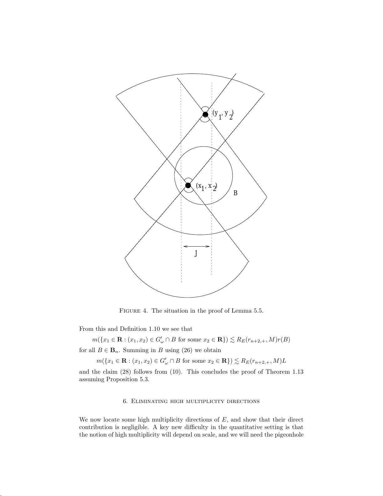
A QUANTIT A TIVE VERSION OF THE BESICOVITCH PR OJECTION THEOREM VIA MUL TISCALE ANAL YSIS TERENCE T AO Abstract. By using a m ultiscale an alysis, we esta blish quant itativ e versions of the Besicovitc h pro jection theorem (almost ev ery pro j ection of a purely un- rectifiable set in the plane of finite length has measure zero) and a standard companion result, namely that an y planar set with at least tw o pro jections of measure zero is purely unrectifiable. W e i llustrate these results b y provid- ing an explicit (but wea k) upper bound on the av erage pro jection of the n th generation of a pro duct Cantor set. 1. Introduction 1.1. The Besico vitc h pro jection theorem. The purp ose of this note is to es- tablish a quantitativ e v ersion of the famo us pro jection theorem of B esico vitch. T o state this theorem we first set o ut some notation. Definition 1.2 (Spherical measure) . Let E ⊂ R 2 , a nd let 0 ≤ r − < r + . The one-dimensional r est ricte d spheric al c ontent S 1 r − ,r + ( E ) of E is defined to b e the quantit y S 1 r − ,r + ( E ) := inf X B ∈ B diam( B ) where the infim um ranges ov er all at most countable co llec tio ns B of op en balls B of ra dius r ( B ) ∈ [ r − , r + ] whic h cover E . The one-dimensional spheric al me asur e S 1 ( E ) is then defined as S 1 ( E ) := lim r + → 0 S 1 0 ,r + ( E ) . A set E ⊂ R 2 is S 1 -me asur able if w e ha ve S 1 ( F ) = S 1 ( F ∩ E ) + S 1 ( F \ E ) for all F ⊂ R 2 . If E is compact, then it is easy to see that S 1 0 ,r + ( E ) = lim r − → 0 S 1 r − ,r + ( E ) and hence (1) S 1 ( E ) = lim r + → 0 lim r − → 0 S 1 r − ,r + ( E ) . It is als o w ell known (see e .g . [4, Ch. 4,5]) that spherica l measure S 1 is compa - rable up to constants with Hausdorff measure H 1 , a nd if E is S 1 -measurable with 1 2 TERENCE T A O S 1 ( E ) < ∞ , then the r estriction d S 1 | E of spherical measure to E is a Radon mea- sure. W e refer the r e a der to [4] for further prop erties o f Hausdorff and spherical measure. Definition 1.3 (F av ard length) . W e endo w the unit circle S 1 ⊂ R 2 with no rmalised arclength measure dσ = d H 1 | S 1 2 π , and the cylinder R × S 1 with the pro duct dm × dσ of Lebe s gue measure and nor malised arclength measure. Given any ( c, ω ) ∈ R × S 1 , we form the dual line l c,ω := { x ∈ R 2 : x · ω = c } , th us R × S 1 can be viewed as a double c over of the affine Gr a ssmanian A (2 , 1 ). Given any Lebesg ue measurable set A ⊂ R 2 × S 1 (whic h one ca n view as the cosphere bundle of R 2 ), w e define the F avar d length F av( A ) of A to b e the quantit y F av( A ) := m × σ ( { ( c, ω ) ∈ R × S 1 : ( l c,ω × { ω } ) ∩ A 6 = ∅} ) . If E ⊂ R 2 , we ado pt the co n v ention F av( E ) := F av( E × S 1 ). R emark 1.4 . The F av a rd length is usually defined (see e.g. [2, p. 357]) for subsets E of R 2 rather than subsets A of R 2 × S 1 , but it will b e c on venien t to gener alise the definition of F av ard length in our arguments beca use most of our analys is s ha ll take place on R 2 × S 1 . F or future reference, w e ma k e the simple observ ations that F av ard length is mono tone a nd subadditiv e, th us (2) max(F av( A ) , F av( B )) ≤ F av( A ∪ B ) ≤ F av( A ) + F av( B ) for all A, B ⊂ R 2 × S 1 . Also if A 1 ⊃ A 2 ⊃ . . . is a nested seq uence of compact subsets of R 2 × S 1 , then we have (3) F av( ∞ \ n =1 A n ) = ∞ \ n =1 F av( A n ) . Definition 1. 5 (Rectifiabilit y) . If F : R → R is a function, w e define the Lipschitz c onstant k F k Lip( R ) := sup x 6 = y | F ( x ) − F ( y ) | | x − y | . W e define a Lipsch itz gr aph in R 2 to be an y set Γ of the for m Γ = { xω 1 + F ( x ) ω 2 : x ∈ R } where ω 1 , ω 2 ∈ S 1 are orthonormal and F : R → R has finite Lipschitz constant. W e say that a set E is pur ely unr e ctifiabl e if S 1 ( E ∩ Γ) = 0 for all Lipsc hitz g r aphs Γ, or equiv alen tly if m ( { x ∈ R : xω 1 + F ( x ) ω 2 ∈ E } ) = 0 for all orthono r mal ω 1 , ω 2 ∈ S 1 and all Lipschitz F : R → R , where m deno tes Leb e s gue measure o n R . W e can no w state the Besicovitc h pr o jection theorem: Theorem 1.6 (Besicovitc h pro jection theorem) . [1, Theorem 6.13] L et E ⊂ R 2 b e an S 1 -me asur able set s u ch that S 1 ( E ) < ∞ and that E is pur el y unr e ctifiable. Then F av( E ) = 0 . As a corollar y of this and (3), we obtain QUANTIT A TIVE BESICOVITC H PROJECT ION THEOREM 3 Corollary 1 .7. L et E ⊂ R 2 b e an S 1 -me asur able set such that S 1 ( E ) < ∞ and that E is pur ely unr e ctifiable. S upp ose also that E = T ∞ n =1 E n for some neste d c omp act sets E 1 ⊃ E 2 ⊃ . . . (in p articular, E is also c omp act). Then lim n →∞ F av( E n ) = 0 . As a n instance of this coro lla ry , let us recall the standard example of the product Cantor set. Example 1.8 (Can tor set) . Let K := { P ∞ n =1 a n 4 − n : a n ∈ { 0 , 3 }} b e the middle- half Cant or set, then K × K has finite S 1 measure and is purely unrec tifiable (see Prop osition 1 .1 6 b elo w), and thus has zero F av ard length b y Theorem 1 .6. If we let K n := { ∞ X k =1 a k 4 − k : a k ∈ { 0 , 3 } for 1 ≤ k ≤ n and a k ∈ { 0 , 1 , 2 , 3 } for k > n } then K × K = T ∞ n =1 K n × K n , and thus by Corollar y 1.7 we have F av( K n × K n ) → 0 as n → ∞ . 1.9. A quantitat iv e Besico vitc h pro jection theorem. The standard pro of of Corollar y 1.7 do es not g iv e a n explicitly quan titative bo und on how quickly F av( E n ) decays to zero. Ev en in the mo del case of the pro duct Cantor set in Example 1.8, a non-trivial upper b ound on F av( K n × K n ) was only established re c e ntly in [7], who established a b ound of the form (4) F av( K n × K n ) ≤ C e − c log ∗ n for some explicit a bsolute constant s C, c > 0, where log ∗ is the inv erse tow er func- tion log ∗ y := min { n ≥ 0 : log ( n ) y ≤ 1 } and lo g ( n ) y is the n th iterated logarithm, thus for instance log (3) y = log log log y . This w eak b ound was strengthened more recently [5] to (5) F av( K n × K n ) ≤ C n − c for s ome explicit a bsolute constants C, c > 0; in the con verse dir e ction, an easy argument esta blishes the low er bound F av( K n × K n ) ≥ c/n for some c > 0, whic h is expe c ted to b e shar p. The argument in [7] also extends to several other mo del examples o f unrectifiable sets, but to the author’s knowledge no qua n titativ e v ersion of Theorem 1.6 in its full generality has appear e d in the literature. This is the main purp ose of the current pap er; we will not quite b e able attain the type o f b ounds in (4) (and certainly not those in (5)), but w e will obtain some explicit b ound nonetheless (see Prop osition 1.21 b elow). These results are p erhaps not so terribly in teresting in their own right, but the a uthor hop es that they do illustrate a g e ner al p oin t, namely that the qualitative (and ostensibly ineffectiv e) arg umen ts coming from infinitary measure theory (e.g. using the Leb esgue differentiation theor em) can often be conv erted in to quan titative (but rather weak) bounds by use of multiscale analysis and the pigeonhole principle (see b elo w). T o ac hieve these goals, we must firs t obtain a quantitativ e v ersion of the unrectifi- abilit y hypothesis. This will b e achiev ed a s follows. 4 TERENCE T A O Definition 1. 1 0 (Rectifiabilit y constant) . Let E be a se t, and let ε, M > 0. W e define the r e ctifiab ility c onstant R E ( ε, r , M ) of E with Lipschitz constant M , error tolerance ε , and scale r to b e the quantit y R E ( ε, r , M ) = sup m ( { x ∈ J : xω 1 + ( F ( x ) + y ) ω 2 ∈ E for so me − ε ≤ y ≤ ε } ) m ( J ) where the supremum ra nges ov er all or thonormal ω 1 , ω 2 ∈ S 1 , all F : R → R with Lipschit z constant k F k Lip( R ) ≤ M , and all interv als J ⊂ R of length at least r . Clearly we hav e the trivial b ound R ( ε, r, M ) ≤ 1. Pure unrectifiability is the assertion that one can improv e upon this bound when ε → 0: Prop osition 1.11 (Equiv alence of qualitative and quan titative unrectifiabilit y) . L et E b e a c omp act subset of R 2 . Then E is pur ely unr e ctifia ble if and only if lim ε → 0 R ( ε, r, M ) = 0 for al l r > 0 and M > 0 . Pr o of. If E is not purely unrectifiable, then E ∩ Γ has p ositiv e S 1 -measure for so me Lipschit z gra ph Γ with s ome Lipschitz constant M , and one easily verifies that R ( ε, r, M ) is then bounded from b elow uniformly in ε for ev ery r > 0 . Now suppose for contradiction that E is purely unrectifiable, but that there exists r > 0 and M > 0 suc h that R ( ε, r, M ) do es not converge to zero as ε → 0. Thus there exists a sequence ε n → 0 a nd δ > 0 suc h that R ( ε n , r , M ) > δ for a ll n . F ro m Definition 1.10, there th us exists o r thonormal ω 1 ,n , ω 2 ,n ∈ S 1 , functions F n : R → R , and in terv als J n ⊂ R with m ( J n ) ≥ r such that m ( { x ∈ J n : xω 1 ,n + ( F n ( x ) + y ) ω 2 ,n ∈ E for some − ε n ≤ y ≤ ε n } ) m ( J n ) > δ. Since E is co mpact, we conclude that J n m ust b e contained in a fixed b ounded set; similarly F n m ust take v alues in a fixed bounded range. By the Bolza no-W eiers tr ass theorem w e ma y th us pass to a subsequence a nd assume that J n conv erges to a fixed in terv al J of length m ( J ) ≥ r , th us m ( J n \ J ) + m ( J \ J n ) → 0. Similarly we ma y assume that ω 1 ,n → ω 1 and ω 2 ,n → ω 2 for some or tho no rmal ω 1 , ω 2 ∈ S 1 . By the Arzela-Ascoli theorem w e can also ass ume that F n conv erges uniformly to so me F , which then has Lipsc hitz norm of at mos t M . F rom the compactness of E , w e see that the set (6) { x ∈ J : xω 1 + F ( x ) ω 2 ∈ E } contains the limit sup erior of the se ts { x ∈ J n : xω 1 ,n + ( F n ( x ) + y ) ω 2 ,n ∈ E for some − ε n ≤ y ≤ ε n } , in the s e ns e that any p oint in the interior of J which lies in infinitely many of the latter, m ust also lie in the for mer. By F ubini’s theo r em we th us see that the set (6) has p o sitiv e measure, cont radicting pure unrectifiability .  One might now naiv ely hope that a quantitativ e version of the Besicovitc h pro- jection theorem would asser t that if E was an S 1 -measurable compact set with some b ounded spherical (or Hausdorff ) measure and bounded diameter, and if w e had some suitable control on the rectifiability constant s, then we would o btain an QUANTIT A TIVE BESICOVITC H PROJECT ION THEOREM 5 explicit non-trivia l upper b ound o n F av( E ), which w ould go to zero as the r ecti- fiabilit y c onstan ts wen t to zero uniformly in E . W e do not know how to achiev e this, and in fac t suspect that such a statemen t is probably false (it is so mewhat analogo us to asking for qua n titativ e bo unds on the a.e. conv ergence in Lebe s gue’s different iation theorem lim r → 0 1 2 r R x + r x − r f ( y ) dy = f ( x ) whic h a re uniform for all bo unded f ; such uniform b ounds are w ell known to b e impo ssible). The problem is that a b ound S 1 ( E ) < L on the spherical measur e of a s e t E is still partially qualitative; it asserts that the spher ica l conten t S 1 0 ,r + ( E ) is ev en tually less than L , but do es not give an effective b ound on the scale r + at which this o ccurs. If how ev er we make these scales explicit, we can in fact r eco ver an effective b ound, which is the main re s ult of this paper: Definition 1.12 (Asymptotic notation) . W e use X . Y or X = O ( Y ) to denote the estimate X ≤ C Y for some absolute co nstan t C > 0 . W e use X ∼ Y to denote the estimates X . Y . X . Theorem 1 .13 (Quantitativ e Besicovitc h pro jection theorem) . L et L > 0 , and let E ⊂ R 2 b e a c omp a ct subset of the un it b al l B (0 , 1) with S 1 ( E ) ≤ L . L et N ≥ 1 b e an inte ger, and s u pp ose that we c an find sc ales (7) 0 < r N , − ≤ r N , + ≤ . . . ≤ r 1 , − ≤ r 1 , + ≤ 1 ob ey ing the fol lowing thr e e pr op erties: • (Uniform length b oun d) F or al l 1 ≤ n ≤ N we have (8) H 1 r n, − ,r n, + ( E ) ≤ L . • (Sc ale sep ar a tion) F or al l 1 ≤ n < N we have (9) r n +1 , + ≤ 1 2 r n, − . • (Unr e ctifiabi lity) F or al l 1 ≤ n < N we have (10) R E ( r n +1 , + , r n, − , 1 r n, − ) ≤ N − 1 / 100 . Then we have F av( E ) . N − 1 / 100 L. Note that by applying (8) at a single sca le n , w e only obtain the trivial b ound F av( E ) ≤ L . The po in t is that we can improve up on this bo und b y using mult iple separated scales , as long as at each scale, E is quantitativ ely unr ectifiable relative to the next finer scale. W e remark tha t the facto rs of 100 can certainly b e low ered (for instance, one can easily replace these factors with 10) but we hav e exag gerated these co nstan ts in order to cla rify the argument (and a lso b ecause these b ounds are in an y even t extremely po or). W e observe that Theorem 1.13 eas ily implies Theorem 1.6. Indeed, for the latter theorem one can quickly reduce to the case when E is co mpact (basically b ecause the r estriction of spherica l measur e to E is a Radon measure, and also becaus e Lemma 5.1 b elo w allows one to neglect sets o f small spherical measure for the 6 TERENCE T A O purp o ses of computing F av a rd length); we can then normalise E to lie in the unit ball B (0 , 1). Giv en any N , one can use (1) and Pro position 1.11 to iter ativ ely construct s c a les (7) ob eying the pr operties in Theorem 1.13, with L set equal to S 1 ( E ) + ε for some ε > 0. Setting N → ∞ we obtain Theorem 1.6. Our pro of is essen tially a finitised version of the one in the b oo k [4] by Ma ttila, and in particular uses essent ially the sa me g eometric ingredients; we give it in Sections 5-9. The main difficulty is to translate the q ualitativ e co mponents o f the arguments in [4] to a quan titative version. F or instance, a fundamen tal fact in qualitative mea sure theory is that countably additive measures are contin uous from below; thus if ( X , µ ) is a measure space and E 0 ⊂ E 1 ⊂ E 2 ⊂ . . . are measurable then µ ( S ∞ n =1 E n ) = lim n →∞ µ ( E n ). W e will rely heavily on the following simple quantit ative version o f this fact. Lemma 1.14 (Pigeonhole principle) . L et ( X , µ ) b e a me asur e sp ac e, and let E 0 ⊂ E 1 ⊂ . . . ⊂ E N b e any se quenc e of me a sur able subsets of X with N ≥ 2 . If 1 / N ≤ ε ≤ 1 / 2 , then t her e exists 0 ≤ n < m ≤ N with m − n ≥ εN such that µ ( E m \ E n ) . εµ ( E N ) . Pr o of. Let k b e the fir st in teger greater than o r equa l to εN . Obser ve that any element of E N belo ngs to a t mos t k + 1 ∼ εN sets of the for m E n + k \ E n for 0 ≤ n ≤ N − k . The claim then follo ws from the pigeonhole principle.  Roughly sp eaking, this lemma will allow us to reduce the size of cer ta in exceptional sets by a n arbitrar y factor ε , at the cost o f reducing the num b er of av ailable scales b y the same factor ε . W e will genera lly apply this lemma with ε equal to s ome power of N − 1 / 100 , ensuring that there ar e always plen ty 1 of scales av ailable. 1.15. A quant itativ e t w o pro jection theorem. In order to a pply the Besi- covitc h pro jection theorem, one of co urse needs to verify the hypothesis of unrec- tifiabilit y; similarly , in o rder to a pply Theorem 1.1 3 , one needs some no n- trivial quantit ative decay rate o n the rectifiability constants R E ( ε, r , M ) as ε → 0 . One such tool to ac hieve the former is the following simple and well-known result, whic h among other things shows that the product Ca n tor set is purely unrectifiable. Prop osition 1.1 6 (Two pro jection theore m) . L et E ⊂ R 2 b e a c o mp act set such that two of its pr oj e ctions E ω := { x · ω : x ∈ E } and E ω ′ := { x · ω ′ : x ∈ E } have me asur e zer o, whe r e ω , ω ′ ∈ S 1 ar e distinct and not antip o dal. Then E is pur ely unr e ctifiab le. Pr o of. Supp ose for con tradiction that E w as not purely rectifiable, th us (after a rotation if necessar y) there exists a Lipschitz graph { ( x, F ( x )) : x ∈ R } such that the (compact) set A := { x ∈ R : ( x, F ( x )) ∈ E } had po sitiv e Leb esgue measure. 1 One could work more efficien tly here by r unning all the pigeonhole argument s “in paral l el” rather than “in series”, as is for instance done i n Section 4 , but this only leads to a modest improv emen t in the final exponents, and also obscures the exposi tion somewhat, so w e hav e c hosen this m ore conceptually simple approac h. QUANTIT A TIVE BESICOVITC H PROJECT ION THEOREM 7 By the Leb esgue differen tiation theorem, almost every x ∈ A is a p oin t of densit y o f A , thus lim r → 0 m ( A ∩ [ x − r, x + r ]) / 2 r = 1. Also, by the Radamacher differentiation theorem, F ( x ) is differentiable for almos t ev ery x . Thus w e can find an x 0 ∈ A which is a po in t o f density and where F has some der iv ative F ′ ( x 0 ). Since ω, ω ′ are distinct and not antipo dal, at leas t one o f the inner pro ducts ω · (1 , F ′ ( x 0 )) a nd ω ′ · (1 , F ′ ( x 0 )) is non-zer o ; without loss of generality we can a s sume ω · (1 , F ′ ( x 0 )) is not zero . It is then not difficult to show that the set { ω · ( x, F ( x )) : x ∈ A, | x − x 0 | ≤ ε } has po sitiv e measur e for all sufficient ly s ma ll ε > 0. But this s et is cont ained in E ω , contradicting the hypothesis.  It is thus na tur a l to ask for a quantitativ e v ersion of the ab o ve pr oposition. Insp ect- ing the ab o ve argument, we see that a pro of of such a qua n titativ e version is likely to r equire some sort of quantitativ e Leb e s gue differentiation theorem and a quan- titativ e Radama cher differentiation theorem. This can in fact b e do ne relatively easily , and leads to the following quan titative version: Theorem 1.17 (Qua n titativ e tw o pro jection theorem) . L et E ⊂ B (0 , 1) b e a c omp act set, and let ω , ω ′ ∈ S 1 b e such that ∠ ( ω , ω ′ ) , ∠ ( ω , − ω ′ ) ∼ 1 , wher e 0 ≤ ∠ ( ω , ω ′ ) ≤ π denotes the signe d angle b etwe en t wo unit ve ctors. S upp ose also that we hav e a se quenc e of sc ales 0 < r N < r N − 1 < . . . < r 1 ≤ 1 with t he fol lowing pr op erties. • (Sc ale sep ar a tion) Each r n is a ne gative p ower of two; in p articular for al l 1 ≤ n < N we hav e (11) r n +1 ≤ 1 2 r n . • (Smal l pr oje ctions) If E ω := { x · ω : x ∈ E } and E ω ′ := { x · ω ′ : x ∈ E } , then we have (12) m ( N r n +1 ( E ω )) , m ( N r n +1 ( E ω ′ )) ≤ r n for al l 1 ≤ n < N , wher e N r ( A ) denotes the op en r -neighb ourho o d of a set A . Then we have R E ( r N , 1 , N 1 / 100 ) . N − 1 / 100 . R emark 1.18 . This theorem gives a non-trivial b ound on the rectifiability co nstan t R E ( ε, r , M ) when r = 1 ; it is a simple matter to resca le this theorem to cov er more general v alues of r , but we will no t do so here. It is also a ro utine matter to deduce Prop osition 1.16 from Theorem 1.1 7 using Prop osition 1.11 and the contin uit y of Leb e s gue measure with resp ect to monotone limits; w e leave the details to the reader as an exer c is e. As befo r e, the exponents 100 can b e impro ved significantly , but we hav e c hosen not to do so in o rder to clarify the structure of the ar gumen t. The pro of of this theorem is a relatively straight forward finitisation of the ar gumen t used to prov e Prop osition 1.16, a nd we give it in Sections 2-4. This simple pro of 8 TERENCE T A O will also serve as a model for the more complicated argument o f the same nature used to prov e Theorem 1 .13. 1.19. Example: the pro duct Cantor s e t. T o illustrate the ab ov e theorems, w e return to the Ca ntor set K × K and its approximan ts K n × K n describ ed in Ex a mple 1.8. W e first use Theo rem 1 .17 to establish a rectifiabilit y b ound: Prop osition 1.20 (Rectifiabilit y bound for pro duct Cantor set) . If n ≥ m > l ≥ 0 and 1 ≤ M ≤ c lo g 1 / 100 ( m − l + 1 ) for some sufficiently smal l absolute c onstant c > 0 , then R K n × K n (2 − m , 2 − l , M ) . lo g − 1 / 100 ( m − l + 1) . Pr o of. By res caling we ma y normalise l = 0. Set E := K n × K n , and let ω = e 1 , ω ′ = e 2 be the standard basis. With the notatio n o f Theo rem 1.17, o ne ea sily verifies that m ( N r ( E ω )) , m ( N r ( E ω ′ )) ∼ r 1 / 2 for all 2 − n ≤ r ≤ 1 (this is basica lly the asse rtion that K is Minko wski dimension 1 / 2). W e ca n th us create a sequence of sca les 2 − m < r N < r N − 1 < . . . < r 1 ≤ 1 ob eying the h yp otheses of Theorem 1.17 provided that N ≤ c lo g m for some suffi- cient ly large c . The claim now fo llo ws from Theorem 1.17.  W e can no w obtain a b ound s omewhat weak er than (4) (and substantially weak er than (5)). Prop osition 1.21 (F av ard b ound for pro duct Cantor set) . If n ≥ 10 0 , then F av( K n × K n ) . (log ∗ n ) − 1 / 100 . Pr o of. Let E := ∂ ( K n × K n ) b e the boundar y of K n × K n . Observe that K n × K n and E ha ve iden tical pro jections and thus hav e iden tical F av ard length. Also o bserv e that S 1 r,r ( E ) . 1 for all 2 − n ≤ r ≤ 1. F r om this a nd Pr o position 1.20, we see that we can find a sequence of sca les (7) ob eying the prop erties needed for Theorem 1.13, with the r j, + = r j, − = 2 m j equal to nega tiv e pow ers of 2 with 0 ≤ m j ≤ n , provided that we can ensure m j +1 − m j ≫ N and (13) m j +1 ≫ 2 C m 100 j for some large constant C . This is pos sible as long as N ≤ c log ∗ n for some sufficient ly small c . The claim now fo llows from Theorem 1.13.  QUANTIT A TIVE BESICOVITC H PROJECT ION THEOREM 9 W e remark that the bound Prop osition 1.20 can b e improved b y using the mac hinery of β -num bers, as dev elop ed b y Jones [3 ] (see also [6]), although this do es not end up significantly improving P ropo sition 1 .21. As w e will not use such impro vemen ts in this pap er, we shall defer these r e s ults to the Appendix. 1.22. Ac kno wledgements. W e thank Y uv al Peres and P eter Jones for encourage- men t, to Peter Jones and Raanan Sch ul for pointing out the use of β -num bers to bo und the rectifiability constants, and John Garnett for corr ections. The a uthor is also indebted to the anon ymous r eferee for many useful commen ts. The author is suppo rted by a gra n t from the Maca rth ur F oundation. 1.23. Organisation of the paper. The paper is or ganised as follows. Sections 2-4 are devoted to the pro of of the quantitativ e analogue of the tw o pro jection theorem (Prop osition 1.1 6 ), namely Theorem 1.17. W e have chosen to cov er this theorem first, ahead of the mo r e difficult quant itative Besicovitch pro jection theo- rem (Theorem 1.13), as the arg umen ts are s omewhat simpler and th us ser v e a s a n in tro duction to the methods used to prov e Theor em 1 .13. The pro of o f Theorem 1 .17 is mo deled on the pro of of Prop osition 1.1 6, but of course with all qualitativ e statements conv erted into quantitativ e ones. An in- sp e c tio n of that pr o of r ev eals three ma jor ing redien ts: the Lebesg ue differen tiation theorem (that establishes p oints of density inside a dense set), the Radamacher different iation theorem (that establishes points of differen tiability for a Lipsc hitz function), and then a simple o bserv a tion that the imag e o f a set under a Lipschitz function will have pos itiv e measure if there exists a point of density o f that set for which the Lipschitz function is differentiable with non-zero deriv ativ e. W e will give quantitativ e analogues of these three facts in Sections 2, 3, 4 resp ectively , thus concluding the pro of of Theorem 1.17. The remaining sections 5- 9 is devoted to the pro of of Theorem 1.13. The arguments broadly follow the standard pro of of the pro jection theorem, as found for instance in [4], and we summarise it as fo llo ws. In Sec tio n 5 we dispos e of the “nor mal” directions - the directions ω and the p oin ts x ∈ E such that E behaves s omewhat like a subset of a Lipschit z graph in the direction ω near x . Becaus e of the unrec- tifiabilit y of E , we exp ect the contribution of these directions to the F av ard length to be small, and this is indeed what is shown in Section 5. The remaining sectio ns ar e dev oted to the more difficult statement that the non- normal directions (in whic h E has large pieces that are orient ed somewhat along the direction ω near x ) also cont ribute a negligible a moun t to the F av ar d length. T o do this one needs to divide the space of non-nor mal dir ections in to further pieces. In Section 6 we dispose of the “high m ultiplicit y” directions - those directions ω a nd po in ts x ∈ E such that the ray from x in dir e c tio n ω intersects E a large n um b er of times. It turns o ut that the bo unds on the length of E will allow us to get a go o d bo und on the contribut ion of this case to the F av a rd length. 10 TERENCE T A O W e are no w left with the directions whose m ultiplicit y is b ounded or zero. It turns out that a scale pigeonholing argument allows one to disp ose of the former (this is done in Section 7), and so it remains to handle the latter case (in whic h E is behaving like a graph in the ω dir ection, alb eit one with unbounded Lipschit z con- stant) . In Section 8 w e use the Hardy-Littlewoo d maximal inequality to eliminate the “high-density strips” of such gra phs - po rtions of the graph which hav e large densit y inside thin r ectangles oriented along ω . After eliminating suc h regions , it turns out that each p oin t x has only a few directio ns ω which are s till contributing to the F av ard length, g iving a small net contribution in all; w e detail this in Section 9. 2. A quantit a tive Lebesgue differentia tion theorem W e now begin the pro of of Theorem 1.1 7. Let E , ω , ω ′ , N , r 1 , . . . , r N be as in that Theorem. F rom the trivial bound R E ( r N , 1 , N 1 / 100 ) ≤ 1 we obtain the claim for N . 1, so w e may take N to b e large. F o r minor no tational r easons it is als o conv enien t to assume (as w e may) that N 1 / 100 is an integer. Using rotation in v ariance and the h yp othesis E ⊂ B (0 , 1), it suffices to show that m ( { x ∈ [ − 1 , 1] : ( x, F ( x ) + y ) ∈ E for some − r N ≤ y ≤ r N } ) . N − 1 / 100 for all F : R → R with Lipschit z constant k F k Lip ≤ N 1 / 100 . Let us th us fix F , and set A := { x ∈ [ − 1 , 1 ] : ( x, F ( x ) + y ) ∈ E for so me − r N ≤ y ≤ r N } . Note that A is clear ly a compact set; our task is to show that (14) m ( A ) . N − 1 / 100 . F r om definition of A w e see that (15) { ( x, F ( x )) · ω : x ∈ A } ⊂ N r N ( E ω ) and similarly with ω replaced by ω ′ . Inspe c ting the pro of of Prop osition 1.16, w e see that the next step should be so me quantit ative version of the Leb esgue differen tiation theorem, which would es tablish plen ty of p oin ts of densit y in A . It turns out that the correct wa y to a c hieve this is to work with discr etised versions of A . F o r any 1 ≤ n ≤ N , we partition [ − 1 , 1 ] in to dyadic interv als of length r n (the endpo in ts may overlap, but these hav e measure zero a nd will play no role). Let A n be the union of all suc h dy adic in terv als which hav e a non-e mpty intersection with A , thu s A ⊂ A N ⊂ . . . ⊂ A 1 ⊂ [ − 1 , 1 ] . Applying Lemma 1 .14 (and re c a lling that N is larg e), we ma y th us find 0 . 1 N ≤ n 0 ≤ 0 . 9 N such tha t the set ∆ A := A n 0 − N − 3 / 100 N \ A n 0 + N − 3 / 100 N QUANTIT A TIVE BESICOVITC H PROJECT ION THEOREM 11 has small Leb esgue measure: (16) m (∆ A ) . N − 3 / 100 . Roughly sp eaking, this will mean that most points in the coarse-scale set A n 0 − N − 3 / 100 N are s till p o in ts o f densit y fo r A n 0 + N − 3 / 100 N all the wa y down to the muc h finer scale n 0 + N − 3 / 100 N . The set A n 0 + N − 3 / 100 N is no t quite as small as A itself, so these a re not p oints of densit y for A , but this set will nevertheless serve as a go o d enough proxy for A for o ur arg umen ts (which will take place at scale s significantly coa rser than r n 0 + N − 3 / 100 N . W e now fix this v alue of n 0 , a nd henceforth shall be working e ntirely in the range of scale indices n ∈ [ n 0 − N − 3 / 100 N , n 0 + N − 3 / 100 N ] ⊂ [1 , N ] . 3. A quantit a tive Rad amac her differentia tion theorem W e co n tin ue to use Prop osition 1.16 as a mo del for our argument. This mo del suggests that the next s tep in the argument should inv olve so me quanti tative v ersion of the Radamacher differentiation theorem. This w e do as follows. Given a ny scale index 1 ≤ n ≤ N , w e can consider the dyadic g rid { j r n ∈ [ − 1 , 1] : j ∈ Z } o f p oint s in [ − 1 , 1], equally separa ted by r n . W e then let F n : [ − 1 , 1 ] → R b e the unique con tinu ous, piecewise linear function which agrees with F on this dy adic grid (th us F n ( j r n ) = F ( j r n )), and is linear on each dy adic interv al [ j r n , ( j + 1) r n ] inside [ − 1 , 1]. Since F has a Lipschitz no rm o f at mos t N 1 / 100 , it is ea sy to see that F n do es also, and furthermore we hav e the uniform approximation (17) k F − F n k L ∞ ([ − 1 , 1]) . N 1 / 100 r n . Also, the deriv ative F ′ n , whic h is defined a lmost everywhere, has an L 2 norm o f O ( N 1 / 100 ), th us 0 ≤ k F ′ n k 2 L 2 ([ − 1 , 1]) . N 2 / 200 . Also, o ne can readily c heck that the differences F ′ n +1 − F ′ n are all or thogonal to eac h other , and to F ′ 1 . Thu s b y Pythagoras’ theorem, k F ′ n k 2 L 2 ([ − 1 , 1]) is an increasing function of n . Specia lis ing to scale indices betw een n 0 − N − 3 / 100 N and n 0 + N − 3 / 100 N , and using the pigeonhole principle, we can thus find a scale n 0 − 0 . 9 N − 3 / 100 N ≤ n 1 ≤ n 0 + 0 . 9 N − 3 / 100 N such that k F ′ n 1 + N − 9 / 100 N k 2 L 2 ([ − 1 , 1]) − k F ′ n 1 − N − 9 / 100 N k 2 L 2 ([ − 1 , 1]) . N − 4 / 100 . In particular we see fro m Pytha g oras’ theor em that (18) k F ′ n 1 + N − 9 / 100 N − F ′ n 1 − N − 9 / 100 N k L 2 ([ − 1 , 1]) . N − 2 / 100 . Roughly speaking , this estimate a sserts that F is “ mostly differen tiable” betw een the co arse scale index of n 1 − N − 9 / 100 and the fine scale index of n 1 + N − 9 / 100 , and will serve as our quantitativ e substitute for the Radamac her differen tiation theorem. 12 TERENCE T A O W e now fix this v alue of n 1 , a nd henceforth shall be working e ntirely in the range of scale indices n ∈ [ n 1 − N − 9 / 100 N , n 1 + N − 9 / 100 N ] ⊂ [ n 0 − N − 3 / 100 N , n 0 + N − 3 / 100 N ] ⊂ [1 , N ] . 4. Conclusion of the argument The scale index n 1 established in the preceding section will no w b e a g o o d place to conduct our analysis. Let us supp ose for contradiction that the conclusio n of Theorem 1 .17 is false, then m ( A ) & N − 1 / 100 . This implies that the set (19) m ( A n 0 − N − 3 / 100 N ) & N − 1 / 100 . W e now lo calise to a relatively large interv a l in A n 0 − N − 3 / 100 N in which A and F are both well-behav ed (this is the quantit ative analog ue of selecting a p oin t x 0 in the pro of of Prop osition 1 .16). F r om (1 9) , (16 ) w e hav e Z A n 0 − N − 3 / 100 N N 2 / 100 1 ∆ A . m ( A n 0 − N − 3 / 100 N ) . Also, from (19), (18) Z A n 0 − N − 3 / 100 N N 3 / 100 | F ′ n 1 + N − 9 / 100 N − F ′ n 1 − N − 9 / 100 N | 2 . m ( A n 0 − N − 3 / 100 N ) . W e concatenate these t w o b ounds together: Z A n 0 − N − 3 / 100 N N 2 / 100 1 ∆ A + N 3 / 100 | F ′ n 1 + N − 9 / 100 N − F ′ n 1 − N − 9 / 100 N | 2 . m ( A n 0 − N − 3 / 100 N ) . The set A n 0 − N − 3 / 100 N is the union of dyadic in terv als of length r n 0 − N − 3 / 100 N , and hence also the union of dyadic interv a ls of leng th r n 1 − N − 9 / 100 N . Thus b y the pi- geonhole principle, w e can find a dyadic I ⊂ A n 0 − N − 3 / 100 N of leng th r n 1 − N − 9 / 100 N , such that Z I N 2 / 100 1 ∆ A + N 3 / 100 | F ′ n 1 + N − 9 / 100 N − F ′ n 1 − N − 9 / 100 N | 2 . m ( I ) . W e fix s uch an interv al I . F ro m the a bov e estimate we hav e (20) m (∆ A ∩ I ) . N − 2 / 100 m ( I ) and (21) Z I | F ′ n 1 + N − 9 / 100 N − F ′ n 1 − N − 9 / 100 N | 2 . N − 3 / 100 m ( I ) . Note that the function F ′ n 1 − N − 9 / 100 N is constant on I , so let us write c := F ′ n 1 − N − 9 / 100 N (this is the analog ue of F ′ ( x 0 ) in the pro of of Prop osition 1 .16); no te that | c | ≤ N 1 / 100 . F r om the h ypo theses o n ω , ω ′ , we see that e ither | (1 , c ) · ω | & 1 QUANTIT A TIVE BESICOVITC H PROJECT ION THEOREM 13 or | (1 , c ) · ω ′ | & 1 . Without loss of generality we may ass ume that the former holds. By reversing the sign of ω if necessar y , we shall assume that (22) t := (1 , c ) · ω & 1 . In view o f (21), (22), w e exp ect the function x 7→ ( x, F ( x )) · ω to b e larg ely increasing on I a t scales r n 1 + N − 9 / 100 N and ab ov e. The plan is to co m bine this with (15) to get some go o d lower b ounds on the size of some neighbo urhoo d of E ω . Let us sub divide I int o S := r n 1 + N − 9 / 100 N /r n 1 − N − 9 / 100 N dyadic interv als J 1 , . . . , J S of leng th r n 1 + N − 9 / 100 N . W e also divide R into disjoint interv als ( K m ) m ∈ Z of leng th 100 N 1 / 100 r n 1 + N − 9 / 100 N . W e then say that a dyadic interv al J j of the former kind r e aches an interv a l K m of the latter kind if we have ( x, F n 1 + N − 9 / 100 N ( x )) · ω ∈ K m for at least one x ∈ J j . Since F n 1 + N − 9 / 100 N has a Lipschitz constant o f at most N 1 / 100 , we see that e a c h J j reaches either o ne o r t w o interv als K m . The function F ′ n 1 + N − 9 / 100 N is constant o n eac h int erv al J j . Let us s a y that an in terv al J j is go o d if | F ′ n 1 + N − 9 / 100 N − c | < t/ 100, and b ad otherwise, where t is the q ua n tit y in (22) . F r om (21) and Chebyshev’s inequality we see tha t at most O ( N − 3 / 100 S ) of the in terv a ls J 1 , . . . , J S are bad. The k ey lemma is Lemma 4 . 1 (Rising sun t yp e lemma ) . L et m ∈ Z . Then at le ast one of the fol lowing statements is true: (i) Ther e ar e at most O ( N 1 / 100 ) intervals J j which re ach K m . (ii) Of al l the intervals J j which r e a ch K m , t he pr o p ortion of those J j which ar e b ad is & N − 1 / 100 . (Se e Figur e 1.) Pr o of. O bserv e that on any go o d in terv al J j , the function x 7→ ( x, F n 1 + N − 9 / 100 N ( x )) · ω is a linear function whose slop e is positive and compara ble to 1 , by (22). On a bad interv al, this function is still linear, but the slop e can hav e either sign and has magnitude O ( N 1 / 100 ). On the other hand, an interv a l K m only has length 100 N 1 / 100 times the length of any of the J j . As a co nsequence, we see that any consecutive string J j , J j +1 , . . . , J j + s of go o d interv als which reach K m can hav e length at most s = O ( N 1 / 100 ). Now consider a maxima l string J j , J j +1 , . . . , J j + s of consecutive interv als whic h reach K m . If this string has length muc h larger than N 1 / 100 , the a bov e discussion shows that at lea s t & N − 1 / 100 of the in terv als in this string must b e bad. If the string has length O ( N 1 / 100 ) and there is a t least one bad in terv al, then clearly & N − 1 / 100 of the in terv als in this string a re bad. The only remaining ca s e is if the string has length O ( N 1 / 100 ) and consists entirely o f go od interv als ; let us call these 14 TERENCE T A O g g g g g g g g g g g g b b b b b b b Figure 1. A graph of the function x 7→ ( x, F n 1 + N − 9 / 100 N ( x )) · ω , and the v ario us in terv a ls J j which reach a certain interv al K m . The go o d in terv a ls J j that reach K m are marked with “ g”; the bad ones are marked with “b”. The fir st and last strings are exceptional strings; the other tw o are not. the “exceptional strings”. Then we see that any exce ptional string , the function x 7→ ( x, F n 1 + N − 9 / 100 N ( x )) · ω ascends mono tonically from b elo w K m to ab o ve K m . Thu s, by the in termediate v alue theo r em, betw een any tw o exceptional strings there m ust b e at least one bad in terv al that touches K m ; thus the num ber of exceptional strings cannot exceed o ne plus the num ber of bad int erv als that touch K m . On the other hand, on all the no n-exceptional strings we hav e seen that & N − 1 / 100 of the in terv als are bad. Since all exceptional strings hav e length O ( N − 1 / 100 ), the claim follows.  Call an interv al K m low multiplicity if case (i) of Lemma 4.1 ho lds (with a suitable choice of implied constant), and high multiplicity otherwise. W e ca ll an interv al J j typic al if it only reaches low m ultiplicit y in terv als K m , and atypic al if it reaches at least one high multipli city in terv al K m . Observe that o f all the at ypical interv als J j that reach an y given high m ultiplicit y int erv al K m , at leas t & N − 1 / 100 of them will be bad. Since every interv al J j reaches either one or t wo interv als K m , we thus see that & N − 1 / 100 of the at ypical in terv als J j are bad. Since the n um b er of bad in terv als is O ( N − 3 / 100 S ), we conclude that O ( N − 2 / 100 S ) of the in terv als J 1 , . . . , J S are atypical. QUANTIT A TIVE BESICOVITC H PROJECT ION THEOREM 15 Let us say that an interv a l J j is A -empty if A ∩ J j = ∅ , and A -nonempty otherwise. Note that if J j is A -empt y , then it is completely contained in ∆ A , thu s fro m (20) w e see that at most O ( N − 2 / 100 S ) of the interv als J 1 , . . . , J S are A -empt y . Combining this with the previo us analysis, we see that all but O ( N − 2 / 100 S ) of the in terv als J 1 , . . . , J S are both typical and A -no nempty; in partiuclar the num ber of typical A -nonempt y in terv a ls is ∼ S . F or an y s uc h typical A -nonempty interv a l J j , we th us ha ve an elemen t x j ∈ A ∩ J j , and the n um b er ( x j , F n 1 + N − 9 / 100 N ( x j )) · ω will lie in a low-m ultiplicit y interv al K m . Since the K m are low-mu ltiplicit y , a simple countin g argument then shows that the n umber of such in terv als K m obtained in this manner must be at least & N − 1 / 100 S . By (15 ) and (17), any such interv a l K m will be con tained in N r n 1 ( E ω ). Th us we s ee that N r n 1 ( E ω ) & N − 1 / 100 S 1 00 N 1 / 100 r n 1 + N − 9 / 100 N & r n 1 − N − 9 / 100 N . But this contradicts (12) if N is la rge eno ugh. This establishes Theorem 1.17. 5. Reduction to a normal component W e now beg in the pr oo f o f Theorem 1.13. The main idea is to split E × S 1 in to a “non-normal” region, which r oughly sp eaking b e haves somewhat lik e a Lipschitz graph a nd so can b e cont rolled by the unrectifiability hypothesis, and a “normal” region whic h will be dealt with by v arian ts of the Leb esgue differen tiation theorem. In this section we handle the non-normal co mp onent, lea ving the no rmal comp onent for later. Let µ be 1-dimensional spherical measure S 1 restricted to E , thus µ is s upported on E a nd µ ( E ) ≤ L . W e let µ × σ be the pro duct measure on E × S 1 , thus (23) µ × σ ( E × S 1 ) ≤ L. The following basic lemma will b e useful for eliminating sev eral error terms: Lemma 5.1. F or any µ × σ -me asur able A ⊂ E × S 1 we hav e F av( A ) . µ × σ ( A ) . Pr o of. By F ubini’s theorem, it suffices to show that m ( { x · ω : ( x, ω ) ∈ A } ) . µ ( x : ( x, ω ) ∈ A } for almost every ω ∈ S 1 . But the map x 7→ x · ω is a contraction. Since µ is the restriction of 1- dimensional spherica l meas ure, the claim follo ws.  Lemma 5.1 already yields the claim when N is bounded, so without loss of g e ner alit y we can assume N to b e larg e, say N ≥ 10 100 . F o r s imilar rea sons we can also take N 1 / 100 to be an in teger. Given any ( x, ω ) ∈ E × S 1 , r > 0, and M > 0 , we define the (double) sector X ( x,ω ) ( r , M ) := { y ∈ R 2 : | y − x | < r ; | ( y − x ) · ω | ≤ 1 M | y − x |} (see Figure 2.) 16 TERENCE T A O x ω r ~ r/M Figure 2. A sector X ( x,ω ) ( r , M ). E Figure 3. The sectors asso ciated to a non-nor ma l pair (left) and a normal pair (rig ht). In this figure E is depicted as connected, but this is of course not the cas e in gener al; for instance one could imagine repla cing E here by a mo derately dense subset. Note that this sector has a “ thic kness” compa rable to r/ M in the ω direction, and so we expect the mea sure µ ( X x,ω ( r , M )) to exceed this quantit y when ω is so meho w “normal” to E . Let us formalise this with a definition: Definition 5.2 (Normal dir ection) . Let 100 < n ≤ N − 100 and let M > 1 0 5 . W e say that a pa ir ( x, ω ) ∈ E × S 1 is n ormal at sc ale n with Lipsc hitz constan t M if we hav e (24) µ ( X x,ω ( r , M / 1 0 4 ) \ X x,ω ( r n +100 , − , M / 1 0 4 )) > N − 1 / 100 r/ M for at least one r n +100 , − ≤ r ≤ r n − 100 , + . W e let Norm n,M ⊂ E × S 1 denote the set of all pairs which a re nor mal a t sca le n and L ips chitz constant M . (See Fig ure 3.) It is easy to v erify that No r m n,M is measurable with respec t to µ × σ . In the next section we shall establish the following somewhat technical res ult. QUANTIT A TIVE BESICOVITC H PROJECT ION THEOREM 17 Prop osition 5.3 (Normal directions negligible) . L et the notation and hyp otheses b e as in The or em 1. 13. Ther e ex ists a sc al e index 100 < n ≤ N − 100 and a Lipschitz c onstant M ≤ 1 /r n − 100 , − such that F av(Norm n,M ( E )) . N − 1 / 100 L. Let us assume Pro position 5.3 for now, and see how it implies Theorem 1 .1 3 . If we let G be the space of “go o d” or “non-normal” directions G := ( E × S 1 ) \ Norm n,M then by (2 ) it suffices to show that F av( G ) . N − 1 / 100 L. F o r each ω , let G ω ⊂ E denote the set G ω := { x : ( x, ω ) ∈ G } ; b y F ubini’s theorem, it thus suffices to show that (25) m ( { x · ω : x ∈ G ω } ) . N − 1 / 100 L for all ω ∈ S 1 . Fix ω . W e fir s t get rid of an exceptional set. By (8) we can find a finite collection B n of op en balls with radius b et ween r n, − and r n, + which cov er E , such that (26) X B ∈ B n r ( B ) . L. If B ∈ B n is s uch a ball, we say that an interv al J ⊂ R is low-density r elative to B and ω if | J | ≤ r n, − and (27) µ ( { x ∈ B ∩ G ω : x · ω ∈ 5 J } ) ≤ 10 10 N − 1 / 100 | J | , where 5 J is the interv a l with the same cen tre as J but fiv e times the length. W e let E ω denote the union of all the sets { x ∈ B ∩ G ω : x · ω ∈ J } generated b y balls B ∈ B n and in terv als J which a re lo w-density relative to B and ω . Lemma 5.4. We have µ ( E ω ) . N − 1 / 100 L . Pr o of. By (8) it suffices to show that µ ( [ J ∈ J B { x ∈ B ∩ G ω : x · ω ∈ J } ) . N − 1 / 100 r ( B ) for all B ∈ B n , where J B is the collection of all the interv als J which are low- densit y relative to B and ω . By monotone con vergence (and the separability of R ), it suffices to sho w this with J B replaced b y any finite sub collection of such interv als. W e can also clea rly restrict atten tion to those J whic h intersect { x · ω ⊥ : x ∈ B } . Using Wiener’s Vitali-type cov ering lemma 2 , we can then cov er this s ubcollection b y 5 J 1 , . . . , 5 J K for so me disjoin t J 1 , . . . , J K in J B which in tersect { x · ω ⊥ : x ∈ B } . But b y hypothesis (27) we ha ve µ ( { x ∈ B ∩ G ω : x · ω ∈ 5 J k } ) . N − 1 / 100 | J k | 2 This lemma asserts that given an y finite collection of balls B 1 , . . . , B n , one can find a sub col- lection B i 1 , . . . , B i K of disjoint balls suc h that the dilates 5 B i 1 , . . . , 5 B i K co ve r S n j =1 B j . 18 TERENCE T A O for a ll 1 ≤ k ≤ K . Since the J k are disjoint , hav e length at most | J k | ≤ r n, − ≤ r ( B ), and in tersect { x · ω : x ∈ B } , w e see that P K k =1 | J k | . r ( B ). Summing the previous estimate in k we obtain the claim.  W e now use ro tational symmetry to normalise ω = e 1 . Let G ′ ω := G ω \ E ω . In view of the ab o ve lemma, we see that to show (25) it suffices to show that (28) m ( { x 1 ∈ R : ( x 1 , x 2 ) ∈ G ′ ω for some x 2 ∈ R } ) . N − 1 / 100 L. W e now make a k ey geometric observ ation (cf. [4, Lemma 15 .1 4]), that G ′ ω is behaving v ery muc h lik e a Lipschitz g r aph: Lemma 5 .5 (Approximate Lipsc hitz prop erty) . L et ( x 1 , x 2 ) , ( y 1 , y 2 ) ∈ G ′ ω b e such that | x 1 − y 1 | + | x 2 − y 2 | ≤ 1 0 r n − 1 , − . Then | x 2 − y 2 | ≤ 1 10 M | x 1 − y 1 | + 1 10 r n +2 , + . (Se e Figur e 4.) Pr o of. Fix ( x 1 , x 2 ) ∈ G ′ ω , and define the set H := { ( y 1 , y 2 ) ∈ G ω : | x 1 − y 1 | + | x 2 − y 2 | ≤ 10 r n − 1 , − } and the quantit y R := sup {| x 2 − y 2 | : ( y 1 , y 2 ) ∈ H } . Clearly R ≤ 10 r n − 1 , − . T o establish the claim, it will suffice (since G ω contains G ′ ω ) to show that R ≤ 1 10 M | x 1 − y 1 | + 1 10 r n +2 , + . Suppose this is not the case, th us (29) 1 10 M | x 1 − y 1 | + 1 10 r n +2 , + < R ≤ 10 r n − 1 , − . By definition of R , we can th us find ( y 1 , y 2 ) ∈ H such that (30) 1 2 R ≤ | x 2 − y 2 | ≤ R ; in particular, from (29) and (30) we ha ve (31) | x 2 − y 2 | ≥ 1 20 M | x 1 − y 1 | , 1 20 r n +2 , + . Fix this ( y 1 , y 2 ). By the non-nor malit y hypo thesis , we ha ve µ (( X ( x 1 ,x 2 ,ω ) ( r , M / 1 0 4 ) \ X ( x 1 ,x 2 ) ,ω ( r n +100 , − , M / 1 0 4 )) ∩ G ω ) ≤ N − 1 / 100 r/ M and µ (( X ( y 1 ,y 2 ,ω ) ( r , M / 1 0 4 ) \ X ( y 1 ,y 2 ) ,ω ( r n +100 , − , M / 1 0 4 )) ∩ G ω ) ≤ N − 1 / 100 r/ M for all r n +100 , − ≤ r ≤ r n − 100 , + , and thus (32) µ ( Y r ∩ G ω ) ≤ 2 N − 1 / 100 r/ M where Y r := ( X ( x 1 ,x 2 ,ω ) ( r , M / 1 0 4 ) \ X ( x 1 ,x 2 ) ,ω ( r n +100 , − , M / 1 0 4 )) ∪ ( X ( y 1 ,y 2 ,ω ) ( r , M / 1 0 4 ) \ X ( y 1 ,y 2 ) ,ω ( r n +100 , − , M / 1 0 4 )) . W e apply this fact with r := 10 0 0 | y 2 − x 2 | ; note that (30), (29), (9) clearly ensure that r lies in the range r n +100 , − ≤ r ≤ r n − 100 , + . QUANTIT A TIVE BESICOVITC H PROJECT ION THEOREM 19 Let J be the in terv a l J := [ x 1 + y 1 2 − 10 | x 2 − y 2 | M , x 1 + y 1 2 + 10 | x 2 − y 2 | M ]. F rom (3 1) we see that [ x 1 , y 1 ] ⊆ J . W e claim the set inclusio n (33) { ( z 1 , z 2 ) ∈ H : z 1 ∈ 5 J } ⊂ Y r . Indeed, if ( z 1 , z 2 ) ∈ H is such that z 1 ∈ 5 J , then | z 2 − x 2 | ≤ R ≤ 2 | x 2 − y 2 | and | z 1 − x 1 + y 1 2 | ≤ 50 M | x 2 − y 2 | , and th us by the triangle inequalit y and (31) (34) | z 2 − x 2 | , | z 2 − y 2 | ≤ 3 | x 2 − y 2 | and | z 1 − x 1 | , | z 1 − y 1 | ≤ 60 M | x 2 − y 2 | . By the triang le inequality , w e either hav e | z 2 − x 2 | ≥ 1 2 | y 2 − x 2 | or | z 2 − y 2 | ≥ 1 2 | y 2 − x 2 | . If | z 2 − y 2 | ≥ 1 2 | y 2 − x 2 | we see fro m (31), (34) that | z 2 − y 2 | ≥ 1 2 | y 2 − x 2 | ≥ 1 120 M | z 1 − y 1 | which implies from choice of r that ( z 1 , z 2 ) ∈ X ( y 1 ,y 2 ,ω ) ( r , M / 1 0 4 ) \ X ( y 1 ,y 2 ) ,ω ( r n +100 , − , M / 1 0 4 ) . Similarly , if | z 2 − x 2 | ≥ 1 2 | y 2 − x 2 | then ( z 1 , z 2 ) ∈ X ( x 1 ,x 2 ,ω ) ( r , M / 1 0 4 ) \ X ( x 1 ,x 2 ) ,ω ( r n +100 , − , M / 1 0 4 ) . In either case we o btain (33). The point ( x 1 , x 2 ) lies in E , and is thus contained in a ball B in B n , whose r adius r ( B ) is at most r n, + . In particular we see from definition of H (and (9)) that B ∩ G ω ⊂ H . Thus from (33) and (32) we hav e µ ( { ( z 1 , z 2 ) ∈ B ∩ G ω : z 1 ∈ 5 J } ) ≤ 1 0 5 N − 1 / 100 | J | / M (say). Compar ing this with (27) we see that J is lo w-density relative to B and ω , and th us ( x 1 , x 2 ) ∈ E ω , contradicting the hypo thesis that ( x 1 , x 2 ) ∈ G ′ ω .  W e now mo dify the sta nda rd pro of o f the w ell-known result that a partially defined real-v alued Lipschitz funct ion extends to a totally defined rea l-v alued Lipschit z function to obtain: Corollary 5.6 (Explicit rectifiability) . L et B ⊂ R 2 b e a b al l of ra dius at most r n, − . Then ther e exists a Lipschitz function F B : R → R of Lipsch itz c onstant at most M such t hat | x 2 − F B ( x 1 ) | ≤ r n +2 , + for al l ( x 1 , x 2 ) ∈ G ′ ω ∩ B . Pr o of. W e may assume that G ′ ω ∩ B is no n-empt y , otherwise there is nothing to prov e. If we then define F ( x ) := sup { y 2 + M | x − y 1 | : ( y 1 , y 2 ) ∈ G ′ ω } then the claim easily follows fro m the previous lemma.  20 TERENCE T A O 0 0 0 1 1 1 0 0 0 1 1 1 0000000000 0000000000 0000000000 0000000000 0000000000 0000000000 0000000000 0000000000 0000000000 0000000000 0000000000 0000000000 0000000000 0000000000 0000000000 0000000000 0000000000 0000000000 0000000000 0000000000 0000000000 1111111111 1111111111 1111111111 1111111111 1111111111 1111111111 1111111111 1111111111 1111111111 1111111111 1111111111 1111111111 1111111111 1111111111 1111111111 1111111111 1111111111 1111111111 1111111111 1111111111 1111111111 0000000000 0000000000 0000000000 0000000000 0000000000 0000000000 0000000000 0000000000 0000000000 0000000000 0000000000 0000000000 0000000000 0000000000 0000000000 0000000000 0000000000 0000000000 0000000000 0000000000 0000000000 0000000000 1111111111 1111111111 1111111111 1111111111 1111111111 1111111111 1111111111 1111111111 1111111111 1111111111 1111111111 1111111111 1111111111 1111111111 1111111111 1111111111 1111111111 1111111111 1111111111 1111111111 1111111111 1111111111 0000000 0000000 0000000 0000000 0000000 0000000 0000000 0000000 0000000 0000000 0000000 0000000 0000000 0000000 0000000 0000000 0000000 1111111 1111111 1111111 1111111 1111111 1111111 1111111 1111111 1111111 1111111 1111111 1111111 1111111 1111111 1111111 1111111 1111111 00000000 00000000 00000000 00000000 00000000 00000000 00000000 00000000 00000000 00000000 00000000 00000000 00000000 00000000 00000000 00000000 00000000 00000000 11111111 11111111 11111111 11111111 11111111 11111111 11111111 11111111 11111111 11111111 11111111 11111111 11111111 11111111 11111111 11111111 11111111 11111111 0000000 0000000 0000000 0000000 0000000 0000000 0000000 0000000 0000000 0000000 0000000 0000000 0000000 0000000 0000000 0000000 0000000 0000000 0000000 1111111 1111111 1111111 1111111 1111111 1111111 1111111 1111111 1111111 1111111 1111111 1111111 1111111 1111111 1111111 1111111 1111111 1111111 1111111 000000000 000000000 000000000 000000000 000000000 000000000 000000000 000000000 000000000 000000000 000000000 000000000 000000000 000000000 000000000 000000000 000000000 000000000 000000000 000000000 000000000 111111111 111111111 111111111 111111111 111111111 111111111 111111111 111111111 111111111 111111111 111111111 111111111 111111111 111111111 111111111 111111111 111111111 111111111 111111111 111111111 111111111 0000 0000 0000 0000 0000 0000 0000 0000 0000 0000 1111 1111 1111 1111 1111 1111 1111 1111 1111 1111 0000 0000 0000 0000 0000 0000 0000 0000 0000 0000 1111 1111 1111 1111 1111 1111 1111 1111 1111 1111 (x , x ) 1 2 (y , y ) 1 2 J B Figure 4. The situation in the proo f of Lemma 5 .5. F r om this and Definition 1.10 we see that m ( { x 1 ∈ R : ( x 1 , x 2 ) ∈ G ′ ω ∩ B for some x 2 ∈ R } ) . R E ( r n +2 , + , M ) r ( B ) for all B ∈ B n . Summing in B using (26) w e obtain m ( { x 1 ∈ R : ( x 1 , x 2 ) ∈ G ′ ω ∩ B for some x 2 ∈ R } ) . R E ( r n +2 , + , M ) L and the claim (28) follows from (1 0). This concludes the pro of of Theorem 1.1 3 assuming Prop osition 5.3. 6. Elimina ting high mul tiplicity directions W e no w lo cate some high multiplicit y directions of E , a nd sho w that their direct contribution is negligible. A key new difficult y in the quanti tative setting is that the notion of high m ultiplicit y will depend on scale, a nd w e will need the pigeonhole QUANTIT A TIVE BESICOVITC H PROJECT ION THEOREM 21 principle (Lemma 1.14) in order to find a fav ourable s cale with whic h to p erform the analysis. Definition 6.1 (High multipl icity lines) . Let 1 ≤ n ≤ N . A line l ⊂ R 2 is sa id to ha ve high multipli city at a sc ale index ≤ n if the s et E ∩ l contains a set of cardinality at least N 1 / 100 which is r n, − -separated, th us any tw o p oints in E ∩ l are separated by a distance of at least r n, − . W e let H n ⊂ E × S 1 to be the set of all po in ts ( x, ω ) ∈ E × S 1 such that the line l x · ω ,ω is hig h multiplicit y a t a scale index ≤ n . Because E is compact, it is not difficult to show that H n is also c o mpact. Also, from (7) we clea r ly hav e the nesting prop erty H 1 ⊂ H 2 ⊂ . . . ⊂ H N ⊂ E × S 1 . Applying (23) a nd Lemma 1.1 4, we may th us find a scale index 0 . 1 N < n 0 ≤ 0 . 9 N near whic h the H n are stable in the sense that (35) µ × σ ( H n 0 + N − 3 / 100 N \ H n 0 − N − 3 / 100 N ) . N − 3 / 100 L. W e no w fix this n 0 and work entirely within the scale indices n ∈ [ n 0 − N − 3 / 100 N , n 0 + N − 3 / 100 N ] ⊂ [1 , N ] . Now we show that near N 0 , the H n hav e negligible F av ard length. In fact w e shall show something slightly stro nger: Definition 6.2 (Angula r neighbourho o ds) . Let F ⊂ E × S 1 and θ > 0 . W e define the θ -angular neighb ourho o d Nb θ ( F ) of F to be the set Nb θ ( F ) := { ( x, ω ) ∈ E × S 1 : ∠ ( ω , ω ′ ) < θ for some ( x, ω ′ ) ∈ F } . W e define the s et (36) ˜ H := Nb r n 0 − N − 3 / 100 N + 10 , − ( H n 0 − N − 3 / 100 N ) and the slightly smaller s et (37) H ′ := Nb 1 2 r n 0 − N − 3 / 100 N + 10 , − ( H n 0 − N − 3 / 100 N ) . Lemma 6.3 ( ˜ H F av a r d-negligible) . We have F av( ˜ H ) . N − 1 / 100 L. R emark 6.4 . This is a qua n titativ e coun terpart of [4, Lemma 1 8.4]. Pr o of. Let us write n − 0 := n 0 − N − 3 / 100 N for brevity . F rom (8) w e can find a collection B of ba lls B with r adius r ( B ) ∈ [ r n − 0 +5 , − , r n − 0 +5 , + ] which cov er E such that (38) X B r ( B ) . L. If a line l x · ω ,ω is hig h m ultiplicit y at a scale index ≤ n − 0 , then by definition it in tersects E in N 1 / 100 po in ts x 1 , . . . , x N 1 / 100 which are r n − 0 , − -separated. Ea c h of 22 TERENCE T A O ω ω ’ x x i x j B i 5B i j 5B j B Figure 5. The situation in the proo f of Lemma 6 .3, not dr a wn to scale. these p oints is con tained in a ba ll B 1 , . . . , B N 1 / 100 in B , where ea c h B i has ra dius r ( B i ) ≤ r n − 0 +5 , + ≤ 1 32 r n − 0 , − , thanks to (7), (9); in particular, the B i are a ll disjoin t. Now let ω ′ ∈ S 1 be such that ∠ ( ω , ω ′ ) ≤ r n − 0 − 10 , − , th us ∠ ( ω , ω ′ ) ≤ 1 32 r ( B i ) by (7), (9). F r om elemen tary geometry (and the fact that x, x 1 , . . . , x N 1 / 100 all lie in B (0 , 1)) w e then see that the line l x · ω ′ ,ω ′ then meets each o f the dilated balls 5 B i (defined as the ball with the same cen tre as B i and five times the radius) in a line segment of length & r ( B i ) (see Figure 5). T o put it another way , w e hav e Z l x · ω ′ ,ω ′ 1 r ( B i ) 1 B i d S 1 & 1 for all 1 ≤ i ≤ N 1 / 100 . Summing this, we conclude that Z l x · ω ′ ,ω ′ X B ∈ B 1 r ( B ) 1 B d S 1 & N 1 / 100 for a ll ( x, ω ′ ) ∈ ˜ H . By F ubini’s theorem, we conclude that for every ω ′ ∈ S 1 we hav e Z R 2 X B ∈ B 1 r ( B ) 1 B d S 1 & N 1 / 100 m ( { x · ω ′ : ( x, ω ′ ) ∈ ˜ H } ) . Applying (38), we obtain m ( { x · ω ′ : ( x, ω ′ ) ∈ ˜ H } ) . N − 1 / 100 L. In tegrating this in ω ′ , we obtain the claim.  QUANTIT A TIVE BESICOVITC H PROJECT ION THEOREM 23 W e define the e x ceptional set ∆ H := H n 0 + N − 3 / 100 N \ H ′ , th us from (35) we ha ve that (39) µ × σ (∆ H ) . N − 3 / 100 L. Because of this, the contribution of ∆ H will be manageable in the sequel. W e make the tec hnical remark that ∆ H is angularly closed, i.e. for any x ∈ E , the set { ω : ( x, ω ) ∈ ∆ H } is closed. 7. Elimina ting positive mul tiplicity directions In the preceding section we obtained t wo sets ˜ H , ∆ H ⊂ E × S 1 of high multip licity which were well controlled. No w w e perfor m another scale refinemen t to a lso control those directions in which the multiplicit y is merely p ositiv e , leaving only the zero- m ultiplicit y directions . Definition 7.1 (Positiv e multiplicit y direction) . Let n 0 − 0 . 9 N − 3 / 100 N ≤ n ≤ n 0 + 0 . 9 N − 3 / 100 N . W e say that a p oin t ( x, ω ) ∈ E × S 1 has p osi tive m u ltipli city at sc ale index n if the line l x · ω ,ω contains a p oint y in E suc h that r n − N − 7 / 100 N , − ≤ | x − y | ≤ r n + N − 7 / 100 N , + . W e let P n ⊂ E × S 1 be the set o f a ll ( x, ω ) which hav e po sitiv e m ultiplicit y at scale index n . Suppos e that ( x, ω ) do es not lie in H ′ ∪ ∆ H , so in par ticular ( x, ω ) do es no t lie in H n 0 + N − 3 / 100 N . A pplying Definition 6.1, w e conclude that l x · ω ,ω contains a t most N 1 / 100 po in ts of E which ar e r n 0 + N − 3 / 100 N , − -separated. Co mparing this with Definition 7.1, we see that ( x, ω ) ca n lie in at most O ( N 1 / 100 N − 7 / 100 N ) of the sets P n . In tegrating this and using (23), w e conclude that X n 0 − 0 . 9 N − 3 / 100 N ≤ n ≤ n 0 +0 . 9 N − 3 / 100 N µ × σ ( P n \ ( ˜ H ∪ ∆ H )) . N 1 / 100 N − 7 / 100 N L. Applying the pigeonhole principle, we can th us find n 0 − 0 . 9 N − 3 / 100 N ≤ n 1 ≤ n 0 + 0 . 9 N − 3 / 100 N such that (40) µ × σ ( P n 1 \ ( H ′ ∪ ∆ H )) . N − 3 / 100 L. Because of this, the cont ribution of P n 1 will be manageable in the sequel. Also observe that P n 1 is closed, and hence P n 1 \ H ′ is angular ly closed in the sense o f the preceding section. Henceforth we fix n 1 , and w ork enti rely within the scale indices n ∈ [ n 1 − N − 7 / 100 N , n 1 + N − 7 / 100 N ] ⊂ [ n 0 − N − 3 / 100 N , n 0 + N − 3 / 100 N ] ⊂ [1 , N ] . 24 TERENCE T A O 8. Elimina ting high density strips W e now p erform a v ar ian t of the analys is of the preceding s e c tions , in order to eliminate the contribution of certain strips { x : x · ω ∈ J } in R 2 which ar e capturing to o muc h of the mass o f µ . Definition 8.1 (High density strips) . Let 1 ≤ n ≤ N . An infinite strip { x ∈ R 2 : x · ω ∈ J } , where ω ∈ S 1 and J is a n interv al, is said to hav e high density if we hav e µ ( { x ∈ E : x · ω ∈ J } ) ≥ N 1 / 100 m ( J ) . W e let D n ⊂ E × S 1 be the set of all points ( x, ω ) ∈ E × S 1 such that the line l x · ω ,ω lies in a high-density str ip { x ∈ R 2 : x · ω ∈ J } whose width m ( J ) is at lea st r n, − . One easily verifies that D n is compact and that D 1 ⊂ D 2 ⊂ . . . ⊂ D N ⊂ E × S 1 . Restricting to s cale indices n b et ween n 1 − 0 . 9 N − 7 / 100 N a nd n 1 + 0 . 9 N − 7 / 100 N , a nd then applying (23) and Lemma 1.1 4 , we can lo cate a scale index n 1 − 0 . 9 N − 7 / 100 N ≤ n 2 ≤ n 1 + 0 . 9 N − 7 / 100 N such that (41) µ × σ ( D n 2 + N − 10 / 100 N \ D n 2 − N − 10 / 100 N ) . N − 3 / 100 L. Let us now fix this n 2 , and work en tirely inside the range of scale indices n ∈ [ n 2 − N − 10 / 100 N , n 2 + N − 10 / 100 N ] ⊂ [ n 1 − N − 7 / 100 N , n 1 + N − 7 / 100 N ] ⊂ [ n 0 − N − 3 / 100 N , n 0 + N − 3 / 100 N ] ⊂ [1 , N ] . Define ˜ D := N r n 2 − N − 10 / 100 N + 10 , − ( D n 2 − N − 10 / 100 N ) and the slightly smaller s et D ′ := N 1 2 r n 2 − N − 10 / 100 N + 10 , − ( D n 2 − N − 10 / 100 N ) W e ha ve an analog ue of Lemma 6.3: Lemma 8.2 ( ˜ D F av a rd-negligible) . We have F av( ˜ D ) . N − 1 / 100 L. Pr o of. By F ubini’s theo r em, it s uffices to show that m ( { x · ω : ( x, ω ) ∈ ˜ D } ) . N − 1 / 100 L for all ω ∈ S 1 . Fix ω ; by rota tio n symmetry we can take ω = e 1 , so we need to s ho w (42) m ( { x 1 : ( x 1 , x 2 , e 1 ) ∈ ˜ D } ) . N − 1 / 100 L. QUANTIT A TIVE BESICOVITC H PROJECT ION THEOREM 25 W e also abbre v iate n − 2 := n 2 − N − 10 / 100 N . Unwrapping the definitions, we see that if ( x 1 , x 2 , e 1 ) ∈ ˜ D , then there exis ts ω ′ ∈ S 1 with ∠ ( ω ′ , e 1 ) ≤ r n − 2 +10 , − and a n in terv al J containing x · ω ′ with m ( J ) ≥ r n − 2 , − such that µ ( { ( y 1 , y 2 ) ∈ E : ( y 1 , y 2 ) · ω ∈ J } ) ≥ N 1 / 100 m ( J ) . F r om (7), (9 ) we have ∠ ( ω ′ , e 1 ) ≤ 1 2 10 m ( J ). Also, ( x 1 , x 2 ) a nd ( y 1 , y 2 ) lie in the unit ba ll. F ro m this, we see that x 1 ∈ 2 J , and furthermore if ( y 1 , y 2 ) ∈ E is such that ( y 1 , y 2 ) · ω ∈ J , then y 1 ∈ 2 J . Thus, if we let µ 1 be the pushforward of the measure µ to R under the pro jection map ( y 1 , y 2 ) 7→ y 1 , w e see that µ 1 (2 J ) ≥ N 1 / 100 m ( J ) . Since 2 J co n tains x 1 , we thus see that the Hardy-Littlewoo d maximal function M µ 1 ( x ) := sup r > 0 1 2 r µ 1 ([ x − r , x + r ]) of µ 1 takes the v a lue & N 1 / 100 on x 1 . O n the other hand, from (23) we see that the total mass µ 1 ( R ) of the pos itiv e measure µ 1 is at most L . The cla im (42) then follo ws from the Hardy-Littlewoo d maximal inequality m ( { x : M µ ≥ λ } ) . 1 λ µ ( R ) for mea sures (see e.g. [4 , Theor em 2.1 9]).  If we define ∆ D := D n 2 + N − 10 / 100 N \ D ′ then from (41) we hav e (43) µ × σ (∆ D ) . N − 3 / 100 L. W e no w define a unified exceptional set ∆ := ∆ H ∪ ( P n 1 \ H ′ ) ∪ ∆ D ; from (39), (40), (43) we have (44) µ × σ (∆) . N − 3 / 100 L. Also, ∆ is ang ularly closed. Beca use of this, the co n tribution of ∆ will b e manage- able in the sequel. 9. Conclusion of the argument Having refined our s e t of s cales suitably , and controlled v arious exc e ptio na l sets, namely t wo large but coarse sets ˜ H , ˜ D , and o ne fine but sma ll set ∆, we are now ready to establish Pro position 5.3. It will suffice to show that F av(Norm n 2 , 10 4 /r n 2 − 200 , − ) . N − 1 / 100 L. In view of Lemma 6.3, Lemma 8 .2, a nd (2), it suffices to show that (45) F av( F ) . N − 1 / 100 L where F is the set F := Norm n 2 , 10 4 /r n 2 − 200 , − \ ( ˜ H ∪ ˜ D ) . 26 TERENCE T A O The key observ ation is that F only consists o f points which a re close to many p oin ts in ∆. Lemma 9.1. L et ( x, ω ) ∈ F . Then the set Ω x,ω := { ω ′ ∈ S 1 : ∠ ( ω , ω ′ ) ≤ 10 4 r n 2 − 200 , − ; ( x, ω ′ ) ∈ ∆ } ⊂ S 1 has me asur e σ (Ω x,ω ) & N − 2 / 100 r n 2 − 200 , − . Pr o of. F ro m Definition 5 .2 we hav e (46) µ ( X x,ω ( r , 1 /r n 2 − 200 , − ) \ X x,ω ( r n 2 +100 , − , 1 /r n 2 − 200 , − )) & N − 1 / 100 rr n 2 − 200 , − for some r n 2 +100 , − ≤ r ≤ r n 2 − 100 , + . Fix this r . Since ∆ is ang ularly closed, Ω x,ω is a co mpact subset of the circle S 1 . Thu s we ca n find a finite num ber o f open ar cs I 1 , . . . , I K in the arc I ∗ := { ω ′ ∈ S 1 : ∠ ( ω , ω ′ ) ≤ 10 5 r n 2 − 200 , − } which cover Ω x,ω and such that (47) σ ( K [ k =1 I k ) . σ (Ω x,ω ) . By enlarg ing these arcs slightly w e can assume that each arc contains at least one po in t in the co mplement of Ω x,ω ; by concatenating overlapping a rcs w e may assume that these arcs are disjoint. Since ( x, ω ) lies in F , it lies outside o f ˜ H , and thus by (37), (36) w e have ( x, ω ′ ) 6∈ H ′ for any ω ′ ∈ I ∗ . A similar argument gives ( x, ω ′ ) 6∈ D ′ for any ω ′ ∈ I ∗ . Suppos e that ω ′ ∈ I ∗ do es not lie in a n y o f the I 1 , . . . , I k , then by the above discussion ( x, ω ′ ) does not lie in ∆, D ′ , or H ′ . In par ticular we see that ( x, ω ′ ) does not lie in P n 1 . This implies that the ray { x + tω ′ : r n 2 +100 , − ≤ | t | ≤ r } do es not in tersect E . Since µ is supp orted on E , we conclude µ ( X x,ω ( r , 1 /r n 2 − 200 , − ) \ X x,ω ( r n 2 +100 , − , 1 /r n 2 − 200 , − )) ≤ K X k =1 µ ( { x + tω ′ : r n 2 +100 , − ≤ | t | ≤ r ; ω ′ ∈ I k } ) and th us by (46) (48) K X k =1 µ ( { x + tω ′ : r n 2 +100 , − ≤ | t | ≤ r ; ω ′ ∈ I k } ) & N − 1 / 100 rr n 2 − 200 , − . On the other hand, giv en an y 1 ≤ k ≤ K , we have b y construction that there exists at lea st one ω k ∈ I k which does not lie in Ω x,ω . In particular this s hows that ( x, ω k ) do es not lie in either D ′ or ∆ D , a nd th us do es no t lie in D n 2 + N − 10 / 100 N . In particular, this shows that µ ( { y ∈ E : y · ω k ∈ J } ) ≤ N 1 / 100 m ( J ) whenever J is an in terv al containing x · ω ′ of length m ( J ) ≥ r n 2 + N − 10 / 100 , − . No w, from elementary geometr y we see that the double sector { x + tω ′ : r n 2 +100 , − ≤ | t | ≤ r ; ω ′ ∈ I k } can be con tained in suc h a strip { y ∈ E : y · ω k ∈ J } with m ( J ) ∼ r σ ( I k ). Thu s m ( { x + tω ′ : r n 2 +100 , − ≤ | t | ≤ r ; ω ′ ∈ I k } ) . N 1 / 100 rσ ( I k ) QUANTIT A TIVE BESICOVITC H PROJECT ION THEOREM 27 I * I 1 2 I x ω ω 1 J 1 Figure 6. A typical situation in the pro of of Lemma 9.1. for all 1 ≤ k ≤ K . Co mparing this with (48), (47) we obtain the claim.  F r om the above lemma, we see that if ( x, ω ) lies in F , then ω lies in the set where the Hardy-Littlewoo d maximal function of the indica tor function of { ω ′ ∈ S 1 : ( x, ω ′ ) ∈ ∆ } on the circle is & N − 2 / 100 . Applying the Hardy-Littlewoo d maximal inequality , we conclude that σ ( { ω : ( x, ω ) ∈ F } ) . N 2 / 100 σ ( ω ′ ∈ S 1 : ( x, ω ′ ) ∈ ∆ } for all x ∈ E . In tegrating this in E we obtain µ × σ ( F ) . N 2 / 100 µ × σ (∆) and the claim (45) then follows from L e mma 5.1 and (44). This concludes the pro of of Theorem 1.13. 28 TERENCE T A O Appendix A. β -numbers a nd quantit a tive unrectifiability The purpose of this app endix is to use the theory of β - n um b ers to improve the bo unds in Propo sition 1.20. Given an y dy adic squa re Q and co mpact set K ⊂ R 2 , let β K ( Q ) denote the quant ity β K ( Q ) := 2 diam( Q ) inf l sup x ∈ K ∩ Q dist( x, l ) where l ranges o ver all lines. Thus for instance β K ( Q ) = 0 when Q ∩ K = ∅ , and also β K ( Q ) ≤ β K ′ ( Q ) whenever K ⊂ K ′ . In [3] it was shown that X Q β K (3 Q ) 2 l ( Q ) . S 1 ( K ) whenever K is compact a nd connected, Q ranges ov er all dyadic squares, l ( Q ) is the length of Q , and 3 Q is the squar e with the same centre as Q but three times the sidelength. In particular, for a Lipsc hitz graph Γ := { xω 1 + F ( x ) ω 2 : − 10 ≤ x ≤ 10 } with k F k Lip ≤ M we see that (49) X Q β Γ (3 Q ) 2 l ( Q ) . 1 + M Prop osition A.1 (Rectifiabilit y b ound for pro duct Cantor set, II) . If n ≥ m > l ≥ 0 then R K n × K n (2 − m , 2 − l , M ) . (1 + M ) / ( m − l ) . Pr o of. O nce again w e can r escale l = 0. By enlarging K n × K n to K m × K m we can also as sume n = m . Let Γ := { xω 1 + F ( x ) ω 2 : − 10 ≤ x ≤ 10 } be a Lipschitz graph with k F k Lip ≤ M , and let E := ( K n × K n ) ∩ Γ, thus E = { xω 1 + F ( x ) ω 2 : x ∈ A } for some closed set A ⊂ R . It then suffices to show that m ( A ) . (1 + M ) /n . W e can assume that m is large, since the claim is trivial otherwise. In view of (49), it th us suffices to show that 1 + X Q β E (3 Q ) 2 l ( Q ) & nm ( A ) . Let 1 ≤ j ≤ n . Then K j × K j consists of 4 j dyadic squar es of sidelength 4 − j ; let E j be the union of all such squar es which in tersect E , th us E ⊂ E n ⊂ . . . ⊂ E 1 . Let 1 ≤ j ≤ n − 1 0, let Q j be one of the squar es in E j , a nd let Q j, 1 , . . . , Q j, 4 10 be the 4 10 dyadic squar es in K j +10 × K j +10 of sidelength 4 − j − 10 which are contained in Q j . F rom elementary geometry we see that if all 4 10 of these s q uares lie in E j +10 , then β E (3 Q j ) ≥ 0 . 01. Viewing this contrap o sitiv ely , we see that if β E (3 Q j ) < 0 . 01 QUANTIT A TIVE BESICOVITC H PROJECT ION THEOREM 29 then E j \ E j +10 contains at least one sq ua re of sidelength 4 − j − 10 contained in Q j . Summing this fact ov er all Q j in E j , w e see that X Q j ⊂ E j : l ( Q j )=4 − j l ( Q j ) . X Q j ⊂ E j : l ( Q j )=4 − j β E (3 Q j ) 2 l ( Q j )+ X Q j +10 ⊂ E j \ E j +10 : l ( Q j +10 )=4 − j − 10 4 − j . A simple countin g arg umen t s ho ws that X Q j ⊂ E j : l ( Q j )=4 − j l ( Q j ) & 4 n m 2 ( E n ) where m 2 denotes tw o-dimensional Lebes gue mea sure. Similarly X Q j +10 ⊂ E j \ E j +10 : l ( Q j +10 )=4 − j − 10 4 − j . 4 n m 2 (( E j \ E j +10 ) ∩ ( K n × K n )) , and th us 4 n m 2 ( E n ) . X Q j ⊂ E j : l ( Q j )=4 − j β E (3 Q j ) 2 l ( Q j ) + 4 n m 2 (( E j \ E j +10 ) ∩ ( K n × K n )) . Summing in j a nd using telescoping series, w e obtain n 4 n m 2 ( E n ) . X Q β E (3 Q ) 2 l ( Q ) + 4 n m 2 ( K n × K n ) . W e can directly compute that 4 m m 2 ( K m × K m ) = 1. Also, E m consists of 4 n m 2 ( E n ) squares of length 4 − n , and the intersection of ea c h such squa re with E contributes a set of measure O (4 − n ) to A . W e thus have m ( A ) . 4 n m 2 ( E n ) and the claim follows.  The estimate in Pr o position A.1 is significan tly s tronger than that in Prop osition 1.20, as the former b ecomes non-trivial as s oon as m − l ≫ M , whereas the latter is only non-trivial for m − l ≫ e C M 100 . How ev er, b oth estimates, when inserted in to Theore m 1.13, g iv e essent ially the same r esult; replacing Prop osition 1.20 b y Pr o position A.1 allows one to r educe the double-exp onent ial in (1 3) to single- exp o nen tial, but after iteration this only affects the (unspecified) implied co nstan t in the final b ound for F av( K n × K n ). Reference s [1] A. Besicovitc h, On the fundamental ge ometric pr op ert ies of line arly me asur a ble plane sets of p oints III , M ath. Ann. 116 (1939) , 349–357. [2] K. F alconer, The geometry of fractal s ets, Cambridge T racts in Mathematics 85 , Cambridge Unive rsity Press, Cambridge-New Y ork, 1986. [3] P . Jones, R e ctifiable sets and t he tr avel ling salesman pr oblem , Inv en t. Math. 10 2 (1990 ), 1–15. [4] P . Mattila, Geometry of Sets and Measures in Euclidean Spaces: F ractals and rectifiability . Camb ridge studies in adv anced mathematics 44 , Cambridge Universit y Press, Cam bridge- New Y ork, 1995. [5] F. Nazarov, Y. Peres, A. V olb erg, prepri n t. [6] K. Okikiolu, Char acterization of subsets of r e cti fiable curves in R n , J. London Math. So c. 46 (1992 ), 336–348. 30 TERENCE T A O [7] Y. P eres, B. Solom y ak, How likely is Buffon ’s ne e dle to fal l ne ar a pl anar Cantor set? , P acific J. M ath. 20 4 (2002) , 473–496. UCLA Dep a r tmen t of Mathema tics, Los Angeles, CA 90095-159 6. E-mail addr ess : tao@@ma th.ucla.ed u