Parallel Pricing Algorithms for Multi--Dimensional Bermudan/American Options using Monte Carlo methods

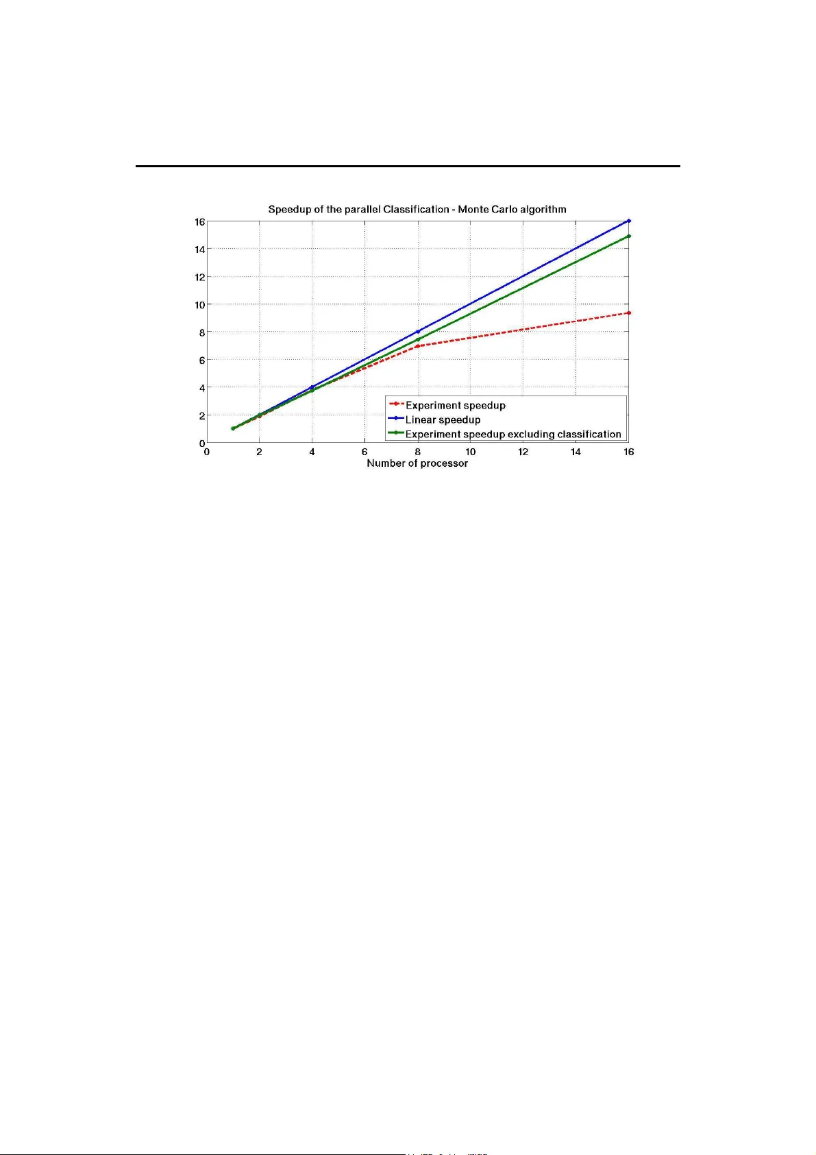
apport   de recherche ISSN 0249-6399 ISRN INRIA/RR--6530--FR+ENG Thèmes COM et NUM INSTITUT N A TION AL DE RECHERCHE EN INFORMA TIQUE ET EN A UTOMA TIQUE P arallel Pricing Algorithms f or Multi–Dimensional Bermudan/American O ptions using Monte Carlo methods V iet_Dung Doan — Abhijeet Gaikwad — Mireille Bossy — Françoise Baude — Ian Stokes-Rees N° 6530 Mai 2008 Unité de recherche INRIA Sophia Antipolis 2004, route des Lucioles, BP 93, 06902 Sophia Antipolis Cedex (France) Téléphone : +33 4 92 38 77 77 — Téléco pie : +33 4 92 38 77 65 P arallel Pr icing Algorithms for Multi–Dimensional Berm udan/American Options using Mon te Carlo metho ds Viet Dung Doan ∗ , Abhijeet Gaikw ad ∗ , Mireille Bossy † , F ran¸ coise Baude ∗ , Ian Stok es-Rees ‡ Th` emes COM et NUM — Sys t ` emes c omm unicants et Syst` emes num ´ er iques Pro jets OASIS et TOSCA Rapp ort de r ec herche n ° 6530 — Mai 2008 — 16 pag e s Abstract: In this pap er we pr esen t tw o paralle l Monte Carlo based algorithms for pr icing m ulti–dimensiona l Bermudan/American options. First a pproach relies o n computation o f the optimal exercise b oundary while the seco nd relies o n cla ssification of co n tinuation and exercise v alues. W e also ev aluate the p erformance of bo th the algorithms in a desktop grid environmen t. W e show the effectiv eness of the prop osed approaches in a heterogeneous computing environmen t, and iden tify scalability constraint s due t o the alg orithmic structure. Key-w ords: Multi–dimensional B e r m udan/America n option, Parallel Distributed Mo n te Carlo metho ds, Grid computing. ∗ INRIA, O ASIS † INRIA, TOSCA ‡ Dept. Biological Chemistry & Molecular Pharmacology , Harv ard Medical Sc hool Algorithmes de P r icing parall ` eles p our des Options Berm u diennes/Am ´ ericaines m ultidimensionnelles par une m ´ etho de de Mon te Carlo R´ esum´ e : Dans ce pa pie r , nous pr´ esentons deux algorithmes de type Monte Ca rlo p our le pricing d’options Ber m udiennes/Am´ ericaines multidim ensionnelles . La pr e miere a pproche rep ose sur le ca lc ul de la fronti ` er e d’exercice, tandis que la seconde rep ose sur la class ification des v aleurs d’exer cice et de contin ua tion. Nous ´ ev aluons les p erformances de s algo r ithmes dans un environnemen t grille. Nous mont rons l’efficacit´ e des appro ches pr o pos´ e e s dans un environnemen t h´ et´ erog` ene. Nous identifions les co n traintes d’´ evolutivit ´ e dues ` a la str ucture algorithmique. Mots-cl´ es : options Berm udiennes/Am´ ericaines m ultidimensionnelles, M´ etho des de Monte Carlo parall´ eles , Grid computing. Par al lel Pricing Algorithms for Multi–Dimensional Bermudan/Americ an Options 3 1 In tro duction Options a r e deriv a tiv e financia l pro ducts which allow buying and selling of risks related to future price v ariations. The option buyer has the right (but not obligation) to purchase (for a call option) or sell (for a put option) any as set in the future (at its exer cise da te) at a fixed pr ice. Estimates of the option price are based o n the well k no wn arbitr a ge pr icing theory: the option price is given by the exp ected v alue of the option payoff at its exercise date. F o r example, the price of a call option is the exp ected v alue of the p ositive part of the differ e nc e b etw een the market v alue o f the underly ing asset and the asse t fixed price at the ex ercise date. The main challenge in this situation is modelling the future asset price and then estimating the payoff exp ectation, which is t ypically done using statistical Mo n te Carlo (MC) simulations and careful selectio n of the sta tic and dynamic par ameters which describ e the mar k et and assets. Some o f the widely used o ptions include American option, where the exer c is e date is v ari- able, and its slight v a riation Bermudan/American (BA) option, with the fairly discretized v ar ia ble exercis e date. Pricing these options with a large num ber o f underlying assets is computationally in tensive and req uires several days o f seria l computationa l time (i.e. on a single pro cessor sy s tem). F or instance, Ibanez and Za patero (2004 ) [1 0] state that pricing the option with five assets ta k es tw o days, which is not desirable in mo dern time critical financial markets. Typical approa c hes for pr ic ing options include the binomia l metho d [5] and MC simulations [6]. Since binomial metho ds ar e not suitable for high dimensio nal op- tions, MC simulations hav e b ecome the corners to ne for simulation of financial mo dels in the industry . Such simulations hav e several adv antages, including ease of implementation and a pplicabilit y to m ulti–dimensiona l options. Although MC sim ulations are p opular due to their “em barr assingly par allel” nature, for simple simulations, allows an almost arbitrar y degree of nea r-p e r fect parallel sp eed-up, their applicability to pricing American options is complex[10], [4], [1 2]. Resea rc hers have pr opo sed several approximation methods to improv e the tr actabilit y of MC simulations. Recen t a dv ances in par allel computing hardware such as multi-core pro cessor s, clusters , compute “clouds” , and large sca le computationa l grids hav e als o attrac ted the interest of the co mputational finance communit y . In literature , there exist a few parallel BA option pricing techniques. Examples include Huang (20 05) [9] or Thu lasir am (200 2) [1 5] which are based on the bino mial la ttice mo de l. How ev er, a very few studies hav e fo cused on paralleliz ing MC metho ds for BA pr icing [16]. In this pap er, we aim to par allelize tw o American option pricing metho ds: the first approach pr opos ed in Ibanez and Zapatero (2004 ) [10] (I&Z) which computes the optimal exer cise b oundary a nd the second prop osed by P icazo (200 2) [8] (CMC) which uses the classificatio n of contin uation v alues. These tw o metho ds in their sequential for m ar e simila r to recursive progra mming so that at a given exe r cise o ppor tunit y they tr ig ger many small independent MC sim ula- tions to compute the contin uation v alues. The optimal stra tegy of an American o ption is to compare the exercise v a lue (intrinsic v alue) with the contin uation v alue (the exp ected cash flow from cont inuing the option cont rac t), then exercis e if the exercise v alue is more v aluable. In the ca se of I&Z Algor ithm the contin uation v alues a re used to para meterize the exercise b oundary whereas CMC Algorithm clas sifies them to provide a character ization of RR n ° 6530 4 Do an, Gaikwad, Bossy, Baude & St okes-R e es the o ptimal exercise b oundary . Later, b oth approa c hes compute the option price using MC simulations based on the computed exercise bo undaries. Our r oadmap is to study b oth the algo r ithms to highlight their p oten tial fo r pa ralleliza- tion: for the different phases, our aim is to ident ify where and how the computation could b e split into indep endent par allel tasks. W e a s sume a master-worker grid pr o gramming mo del, where the master no de splits the co mputation in such tasks and a s signs them to a set of work er no des. Later, the master also collects the par tial results pro duced by these workers. In particular, we in vestigate par a llel BA options pricing to significantly r educe the pr icing time by harness ing the computational p ow er provided by the computational grid. The pap er is or g anized as follows. Sections 2 and 3 fo cus on tw o pricing metho ds and are structured in a s imilar wa y: a brief int ro duction to present the metho d, sequential follow ed by parallel algor ithm and per fo rmance ev aluation concludes each section. In section 4 w e present o ur co nclusions. 2 Computing optimal exercise b oundary algorithm 2.1 In tro duction In [10], the authors pr opo se an option pricing metho d tha t builds a full exer c is e bo undary as a p olynomia l curve whose dimension depe nds on the num b er of under lying assets. This algorithm co nsists o f t wo phases. In the first phase the exercise bo undary is parameter ized. F o r para meterization, the a lg orithm uses linear in terp olation or re g ression of a quadratic or cubic function at a given exercise o pp ortunity . In the s e cond phase, the option pr ice is computed using MC simulations. These simulations are run until the price tra jectory reaches the dynamic bo undary co mputed in the firs t phase. The main adv ant age of this metho d is that it provides a full parameter ization of the exercise b oundary and the exercise rule. F or Amer ican o ptio ns, a buyer is mainly concerned in thes e v alues as he can decide at ease whether or no t to ex ercise the option. At each exe r cise da te t , the optimal exercis e po in t S ∗ t is defined by the following implicit condition, P t ( S ∗ t ) = I ( S ∗ t ) (1) where P t ( x ) is the price of the Amer ican option on the p erio d [ t, T ], I ( x ) is the e xercise v alue (in trinsic v a lue ) of the option and x is the a sset v a lue a t opp ortunity date t . As explaine d in [10], these optimal v alues stem fr om the mono tonicit y and conv exity of the price function P ( · ) in (1). These ar e general prop erties satisfied by mo st o f the deriv ative securities s uc h as maximum, minimum or geometric av erage basket options. How ever, for the problems where the monotonicity and conv exity of the price function can not be easily established, this algo rithm has to b e revisited. In the following section we briefly discuss the sequential algorithm follow ed by a prop osed pa r allel solutio n. INRIA Par al lel Pricing Algorithms for Multi–Dimensional Bermudan/Americ an Options 5 2.2 Sequen t ial Boundary Computation The alg o rithm pr opos ed in [10] is us ed to compute the exer cise b oundary . T o illustra te this approach, we cons ider a call BA option on the maximum of d assets mo deled by Geometric Brownian Mo tio n (GBM). It is a standar d exa mple for the multi–dimensional BA option with maturity date T , constant interest rate r and the price of this o ptio n at t 0 is given as P t 0 = E (exp ( − rτ )Φ( S τ , τ ) | S t 0 ) where τ is the optima l sto pping time ∈ { t 1 , .., T } , defined as the first time t i such that the underlying v alue S τ surpasses the optimal exe r cise b oundary at the o ppor tunity τ otherwise the o ption is held until τ = ∞ . The pay off at time τ is defined as fo llo ws: Φ( S τ , τ ) = (max i ( S i τ ) − K ) + , where i = 1,.., d , S is the underly ing ass et price vector and K is the strike price. The parameter d has a stro ng impact on the complex it y of the a lgorithm, except in some cases as the average options where the num b er o f dimensio ns d ca n b e easily reduced to one. F or an optio n on the maximum of d assets there are d separate exer cise regions which a re characteriz e d by d b oundaries [10]. These b oundaries are mono tonic a nd smo oth curves in R d − 1 . The algor ithm uses backward r ecursive time progr amming, with a finite num ber of exer c ise opp ortunities m = 1 , ..., N T . Each b oundary is computed by regres s ion o n J num b ers of b oundary p oints in R d − 1 . At each given opp ortunity , these optimal b oundary p oin ts are co mputed using N 1 MC simu lations. F urther in cas e o f an option on the ma xim um of d underly ing a ssets, fo r each a sset the b oundary p oints ar e co m- puted. It takes n itera tio ns to converge each individual p oin t. The co mplexit y o f this step is O  P N T m =1 d × J × m × N 1 × ( N T − m ) × n  . Aft er estimating J optimal b oundary p oints for each ass et, d regress ions are p erformed ov er these p oints to get d execution b oundaries. Let us a ssume that the complexity of this step is O ( N T × reg ression ( J )), where the com- plexity of the regr ession is assumed to b e constant. After co mputing the b oundaries at all m ex ercise opp ortunities, in the second phase, the price of the option is computed us- ing a standard MC sim ulation o f N pa ths in R d . The complexity of the pricing phase is O ( d × N T × N ). T hus the total complexity of the a lgorithm is as fo llo ws, O  P N T m =1 d × J × m × N 1 × ( N T − m ) × n + N T × r eg r e ssion ( J ) + d × N T × N  ≈ O  N 2 T × J × d × N 1 × n + N T × ( J + d × N )  F o r the p erformance b enc hmarks, we use the same simulation pa rameters as given in [10]. Consider a call BA option o n the maximu m of d assets with the following configura tion. K = 100, inter est r ate r = 0.05 , volatility r ate σ = 0.2 , dividend δ = 0.1 , J = 1 28, N 1 = 5 e 3, N = 1 e 6, d = 3, N T = 9 and T = 3 years. (2) The sequential pricing o f this optio n (2) takes 4 0 min utes. The distribution of the total time for the different phases is shown in Figure 1. As can b e seen, the data g eneration phase, which simulates and calculates J o ptimal b oundary p oin ts, consumes mos t of the computational RR n ° 6530 6 Do an, Gaikwad, Bossy, Baude & St okes-R e es time. W e b elieve that a par a llel appr o ach to this a nd o ther pha s es could dramatically reduce the computatio nal time. This inspires us to investigate a pa rallel appro ach for I&Z Algorithm which is presented in the following section. The numerical r esults that we shall provide indicate that the prop osed parallel so lution is mor e efficient compar ed with the ser ial algorithm. 2.3 P arallel approac h In this section, a simple parallel approa c h for I&Z Alg orithm is presented and the pseu- do code for the sa me is given in Algo rithm 13. This approach is inspired from the solution prop osed by Muni T oke [16], though he presents it in the co ntext of a low–order homo ge- neous par a llel cluster . The a lgorithm consists of tw o pha ses. The first par allel pha se is bas ed on the following obser v ation: for each of the d bounda ries, the computation of J o ptima l bo undary p oints at a given exercise date ca n b e s imulated indep enden tly . The optimal exer - Algorithm 1 Parallel Iba nez and Zapatero Alg o rithm 1: [g lp] Genera tion of the J “Go o d L attic e Points” 2: for t = t N T to t 1 do 3: for d i = 1 to d do 4: for j = 1 to J i n parallel do 5: [calc] Computation of a b oundary p oin t with N 1 Monte Carlo simulations 6: end for 7: [reg] Regressio n of the exercise b oundary . 8: end for 9: end for 10: for i = 1 to N in parallel do 11: [mc] Computatio n of the par tial option price. 12: end for 13: Estimation of the final optio n pr ic e by merg ing the par tial pric es. cise b oundaries from o pportunity da te m back to m − 1 a re computed as follows. Note that at m = N T , the b oundary is known (e.g. for a call o ption the b oundary at N T is defined as the strike v alue). Ba c kward to m = N T − 1, we hav e to estimate J optimal p oints from J initial go o d lattice p oint s [10], [7 ] to r egress the b oundary to this time. The r egression of R d → R d is difficult to achiev e in a reas onable a moun t of time in case o f large num b er of tr aining p oints. T o decrea se the size of the tra ining set we utilize “Go o d La ttic e Points” (GLPs) as descr ibed in [7],[14], and [3]. In par ticula r case o f a call on the maximum of d assets, only a regr ession of R d − 1 → R is needed, but we r epea t it d times. The Algorithm 13 c omputes GLPs using either SSJ librar y [11] or the quantification nu mber sequences as pr e sen ted in [1 3]. SSJ is a J a v a libra ry for sto chastic simulation and it computes GLP s as a Quasi Monte Carlo s e quence such as Sob ol o r Hamilton sequences. The algorithm can also use the num be r sequences readily av ailable at [1]. These sequences are INRIA Par al lel Pricing Algorithms for Multi–Dimensional Bermudan/Americ an Options 7 generated using an optimal qua dr atic quantizer of the Gaussian distribution in mor e than one dimension. The [calc] phase of the Algorithm 13 is embarrass ingly pa rallel a nd the J b oundary po in ts are equa lly distributed among the computing no de s . At each no de, the algorithm s im ulates N 1 paths to compute the approximate po in ts. Then Newton’s itera tions metho d is used to conv erge a n individual a pproximated point to the optimal bo undary po in t. After computing J optimal b oundary p oints, these p oin ts ar e colle cted by the master no de, for sequential regression of the exercis e boundary . This no de then r epeats the sa me proc edure for every date t , in a recursive way , until t = t 1 in the [reg] phase. The [calc] phase provides the exact o ptimal exer cise b oundary a t every opp ortunity date. After computation of the b oundary , in the last [mc] pha se, the option is priced using parallel MC simulations as shown in the Algorithm 13. 2.4 Numerical results and p erformance In this s ection w e present per formance and accura cy re sults due to the par allel I&Z Algo- rithm descr ib ed in Algo rithm 13. W e price a basket BA call option on the maxim um o f 3 assets as given in (2). The star t prices fo r the assets are v a r ied as 90, 100, and 110. The prices estimated by the algor ithm are pr esen ted in T able 1. T o v alidate our results we com- pare the estimated prices with the prices men tioned in Andersen and Broadies (1997) [2]. Their results a r e repr oduced in the column lab eled a s “Binomial” . The last column of the table indicates the err ors in the estimated prices. As we can see, the estimated option pr ices are close to the desir e d prices by a cceptable marg inal erro r and this er ror is repr e sen ted by a desirable 95% confidence interv al. As ment ioned earlier , the algo rithm relies o n J num ber of GLPs to effectively compute the o ptima l b oundary p oin ts. Later the par ameterized b o undary is reg ressed ov er these po in ts. F or the BA option on the maximum de s cribed in (2), Muni T o ke [16] notes that J smaller than 128 is not sufficient and prejudices the option price. T o observe the effect of the num ber of optimal b oundary p oints on the accura c y of the estimated pr ice, the num b er of GLPs is v aried as shown in T able 2. F or this exp eriment , we set the star t price of the option as S 0 = 90. The table indicates that incre asing num b er of GLPs has neglig ible impact on the acc uracy of the estimated price. How ever, we obse r v e the linear increa se in the computational time with the increa se in the num b er of GLPs. [INSER T T ABLE 1 HE RE] T o ev a luate the a ccuracy o f the computed prices by the paralle l a lgorithm, we obtained the numerical results with 16 pro cess o rs. Fir st, let us obser v e the effect of N 1 , the n umber of simulations r equired in the first phase of the algo r ithm, on the computed o ption price . In [16], the author co mmen ts tha t the large v alues of N 1 do not affect the acc ur acy of o ption price. F or these exp erimen ts, we set the n umber o f GLP s, J , as 12 8 a nd v ary N 1 as shown in T able 3. W e can clea rly obser v e that N 1 in fact ha s a strong impact on the ac curacy of the computed option pric es: the computationa l err or decr eases with the increased N 1 . A large v alue of N 1 results in more accurate b oundary points, hence more accur ate exercis e bo undary . F urther, if the exercise b oundary is a ccurately computed, the res ulting option prices are m uch clos er to the true price. How ever this, as we can see in the third co lumn, RR n ° 6530 8 Do an, Gaikwad, Bossy, Baude & St okes-R e es S i 0 Option Price V a r iance (95% CI) Binomial Error 90 11.254 153.85 7 (0.02 4) 11.29 0.036 100 18.378 192.54 0 (0.03 1) 18.69 0.312 110 27.512 226.33 2 (0.03 5) 27.58 0.068 T a ble 1: Pr ice o f the call BA on the maximum of three a ssets ( d = 3, with the sp ot price S i 0 for i = 1 , .., 3) using I&Z Algo rithm. ( r = 0 . 0 5, δ = 0 . 1 , σ = 0 . 2, ρ = 0 . 0, T = 3 and N = 9). The binomial v alues are r eferred as the true v alues. J Price Time (in minute) Error 128 11.254 4.6 0.036 256 11.258 8.1 0.032 1024 11.26 3 29.5 0.027 T a ble 2: Impa c t of the v alue of J on the results of the maximum on three a ssets option ( S 0 = 90). The binomial price is 1 1.29. Running time on 16 pro cess ors. N 1 Price Time (in minute) Error 5000 11.254 4.6 0.036 10000 11.262 6.9 0.028 10000 0 11.276 3 5.7 0.014 T a ble 3: Impact of the v alue of N 1 on the r e sults of the max im um on three assets option ( S 0 = 90). The binomial price is 1 1.29. Running time on 16 pro cess ors. comes at a cost of increased computational time. The I&Z algorithm highly relies on the accuracy and the conv ergenc e ra te o f the o ptimal b oundary po in ts. While the former a ffects the accuracy o f the option price, the later a ffects the sp eed up o f the algor ithm. In each iteration, to co n verge to the optimal b oundary p oin t, the algo r ithm star ts with an arbitrar y po in t with the strike price K o ften as its initial v alue. The algorithm then uses N 1 random MC paths to s imulate the approximated p oint. A co n vergence criter ion is used to optimize this approximated p o in t. The simulated p oint is assumed to b e optimal when it satisfies the following co ndition, | S i, ( simulated ) t n − S i, ( initial ) t n | < ǫ = 0 .01, where the S i, ( initial ) t n is the initial po in t at a given o pportunity t n , i = 1 ..J a nd the S i, ( simulated ) t n is the p oint sim ulated by using N 1 MC simulations. In cas e, the co ndition is not satisfied, this pro cedure is rep eated and now with the initial p oint a s the newly simulated p oint S i, ( simulated ) t n . Note that the nu mber o f iterations n , requir ed to r each to the optimal v alue, v a ries dep ending o n the fixed precision in the Newton pr ocedur e (for ins tance, with a pr e cision ǫ = 0 . 0 1, n v aries from 30 to 6 0). W e observed that not all bounda ry p oints take the same time for the conv erg ence. INRIA Par al lel Pricing Algorithms for Multi–Dimensional Bermudan/Americ an Options 9 Some p oint s co n verge fas ter to the o ptimal bounda ry p oints while some ta k e longe r than usual. Since the algo rithm has to wait until all the p oints are o ptimized, the slow er p oints increase the computational time, thus reducing the efficiency o f the parallel a lgorithm, see Figure 2 . Data generation 77.90% Regression 0.01% Monte Carlo simulation 22.09% Figure 1: The time distribution for the sequential o ptima l e xercise bounda ry computation algorithm. The total time is ab out 4 0 minutes. 3 The Classification and Mon te Carlo algorithm 3.1 In tro duction The Monte Ca rlo approaches for BA option pricing ar e usua lly ba sed on contin uation v alue computation [12] or contin uation regio n estimation [8], [10]. The option holder decides either to execute or to contin ue with the current option contract based on the computed asse t v alue. If the asse t v a lue is in the exercise region, he exec utes the option otherwise he contin ues to hold the option. Denote that the asset v alues which b elong to the exercise region will form the exercise v alues and r est will belo ng to the co n tinuation r egion. In [8] P icazo et al. pro- po se an algo rithm bas ed on the observ ation that at a given exercise o ppor tunit y the option holder ma k es his decision based o n whether the sig n of ( e xer cise v al ue − continuation v al ue ) is pos itiv e or negative. The a uthor fo cuses o n estimating the contin uation region and the exercise regio n by characterizing the exe r cise bo undary based on these signs . The classifi- cation algor ithm is used to ev alua te such sign v alues a t each opp ortunity . In this section we brie fly desc r ibe the sequential a lgorithm describ ed in [8] and pr o pos e a pa rallel approa c h follow ed by p erformance b enc hmarks . RR n ° 6530 10 Do an, Gaikwad, Bossy, Baude & St okes-R e es Figure 2: Sp eedup of the par allel I&Z Algo rithm. 3.2 Sequen t ial algorithm F o r illustration let us consider a BA o ption on d underlying assets mo deled b y Geo metric Brownian Motion (GBM). S t = ( S i t ) with i = 1 , .., d . The optio n price at time t 0 is defined as follows: P t 0 ( S t 0 ) = E (exp ( − rτ ) Φ( S τ , τ ) | S t 0 ) where τ is the optimal stopping time ∈ { t 1 , .., T } , T is the maturity date, r is the constant int erest rate and Φ( S τ , τ ) is the pay off v a lue at time τ . In case o f I&Z Algor ithm, the optimal stopping time is defined when the underly ing a sset v a lue cr osses the exercise b oundary . The CMC algor ithm defines the stopping time whenever the underlying a s set v alue makes the sign of ( exerc i se v al ue − continuation v al ue ) p ositive. Without los s of g enerality , a t a given time t the BA optio n price on the per io d [ t, T ] is given by: P t ( S t ) = E (exp ( − r ( τ − t ))Φ( S τ , τ ) | S t ) where τ is the o ptimal stopping time ∈ { 1 , .., T } . Let us define the difference b etw een the pay off v alue and the option pr ice at time t m as, β ( t m , S t m ) = Φ( S t m , t m ) − P t m ( S t m ) where m ∈ { 1 , .., T } . The option is exe r cised when S t m ∈ { x | β ( t m , x ) > 0 } which is the ex ercise reg ion, a nd x is the sim ulated underlying asset v alue, other wise the option is contin ued. The goal of the a lgorithm is to determinate the function β ( · ) for every oppor tunit y INRIA Par al lel Pricing Algorithms for Multi–Dimensional Bermudan/Americ an Options 11 date. How e v er, w e do not need to fully parameteriz e this function. It is enough to find a function F t ( · ) such that sig nF t ( · ) = sig nβ ( t, · ). The algo rithm consists of tw o phases. In the firs t phas e, it a ims to find a function F t ( · ) having the same s ign a s the function β ( t, · ). The AdaBo ost or Lo gitBo ost algo rithm is used to characterize these functions. In the sec o nd phase the option is pr iced by a standard MC simulation by taking the adv a ntage of the character iz a tion of F t m ( · ), so for the ( i ) th MC simulation we get the o ptimal stopping time τ ( i ) = min { t m ∈ { t 1 , t 2 , ..., T }| F t ( S ( i ) t ) > 0 } . The ( i ) is not the index o f the num b er of assets. Now, consider a call BA option on the maximum of d underlying asse ts where the pay off at time τ is defined as Φ( S τ , τ ) = (max i ( S i τ ) − K ) + with i = 1 , .., d . During the first phase of the a lgorithm, at a g iv en opp ortunity date t m with m ∈ 1 , ..., N T , N 1 underlying price vectors sized d are simulated. The simulations ar e p erformed r ecursively in backw ard from m = T to m = 1. F rom each pr ice p oint, a nother N 2 paths ar e simulated from a given opp ortunit y date to the maturity date to c ompute the “small” B A o ption pr ic e at this opp ortunit y (i.e. P t m ( S t m )). At this step, N 1 option prices rela ted to the o pp ortunity date are computed. The time step co mplexit y of this step is O ( N 1 × d × m × N 2 × ( N T − m )). In the classifica tion phase, we use a tr aining set of N 1 underlying price p oints and their corres p onding o ption pr ices a t a given opp ortunity date. In this step, a non–par ametric regres s ion is done on N 1 po in ts to characterize the exercise b oundary . This first phas e is rep eated for each opp ortunit y date. In the second phase, the option v alue is computed by simulating a lar ge num b er, N , of standar d MC simulations with N T exercise o pportunities. The complexity of this pha se is O ( d × N T × N ). Thus, the total time steps requir ed for the algorithm can b e given by the following fo rm ula, O  P N T m =1 N 1 × d × m × N 2 × ( N T − m ) + N T × cl assif ication ( N 1 ) + d × N T × N  ≈ O  N 2 T × N 1 × d × N 2 + N T × ( N 1 + d × N )  where O ( cl assif ication ( · )) is the complexity of the classification phase and the details of which ca n be found in [8]. F or the s imulations, we use the same option parameters a s describ ed in (2), taken from [10], and the parameters for the classification can b e found in [8]. K = 1 00, inter est r ate r = 0.05 , volatility r ate σ = 0.2 , dividend δ = 0.1 , N 1 = 5 e 3, N 2 = 500 , N = 1 e 6, d = 3 N T = 9 and T = 3 years. (3) Each of the N 1 po in ts of the training set acts as a seed which is further used to simulate N 2 simulation paths. F rom the ex e r cise opp ortunity m backw ard to m − 1, a Br o wnian motion bridge is used to simulate the pr ice of the under ly ing asset. The time dis tribution of each phase of the s equen tial algo rithm for pricing the option (3 ) is shown in Figure 3. As we can see fro m the figure, the most computationally in tensive part is the data generation phase which is used to compute the option prices r equired for class ification. In the following section we present a pa rallel appr o ach for this and res t of the phas e s of the a lgorithm. RR n ° 6530 12 Do an, Gaikwad, Bossy, Baude & St okes-R e es 3.3 P arallel approac h The Algor ithm 10 illustrates the parallel a pproach based o n CMC Algo r ithm. At t m = T we gener ate N 1 po in ts o f the price of the underlying as sets, S ( i ) t m , i = 1 , .., N 1 then apply the Br ownian bridge simulation pro cess to get the price at the backward da te, t m − 1 . F or simplicity we a ssume a master–worker prog ramming mo del fo r the parallel implementation: the master is resp onsible for allo cating indep endent tasks to workers a nd for co llecting the results. The master divides N 1 simulations into n b tasks then distr ibutes them to a nu mber of work ers. Thus ea c h worker ha s N 1 /nb po in ts to simulate in the [ calc] phas e . Each w or ker, further, simulates N 2 paths for ea c h p oint from t m to t N T starting a t S ( i ) t m to compute the option pr ice related to the opp ortunity da te. Next the work er calculates the v alue y j = ( exerci se v al ue − continuati on v al ue ), j = 1 , .., N 1 /nb . The master c ollects the y j of these nb task s from the work ers and then classifies them in order to return the characterization mo del of the as soc ia ted exercise b oundary in the [class ] phase. F o r the Algorithm 2 Parallel Cla ssification and Mo nte Carlo Algor ithm 1: for t = t N T to t 1 do 2: for i = 1 to N 1 in parallel do 3: [calc] Computation of tra ining p oints. 4: end for 5: [class] Classificatio n using b oo s ting. 6: end for 7: for i = 1 to N i n parallel do 8: [mc] The partial option price computatio n. 9: end for 10: Estimation of the final optio n pr ic e by merg ing the par tial pric es. classification phase, the master do es a non-pa rametric r egression with the set ( x ( i ) , y ( i ) ) N 1 i =1 , where x ( i ) = S ( i ) t m , to get the function F t m ( x ) describ ed ab ov e in Section (3.2). The alg orithm recursively rep eats the s ame pro cedure fo r earlier time interv als [ m − 1 , 1]. As a r esult w e obtain the characterization o f the b oundaries, F t m ( x ), at every opp ortunit y t m . Using these bo undaries, a standard MC simulation, [mc] , is use d to estimate the option price. The MC simulations are distributed a mong work ers such that each work er has the entire characterization b oundary information ( F t m ( x ) , m = 1 , .., N T ) to compute the partial option price. The mas ter la ter mer ges the par tia lly computed pr ices a nd estimates the fina l optio n price. 3.4 Numerical results and p erformance In this s ection we prese n t the numerical and p erformance results of the para lle l CMC Algo- rithm. W e fo cus o n the standa r d e xample of a call option o n the maximum of 3 assets as given in (3). As it can b e se en, the e s timated prices ar e e q uiv alent to the r e ference prices INRIA Par al lel Pricing Algorithms for Multi–Dimensional Bermudan/Americ an Options 13 S 0 Price V a r iance (95% CI) Binomial Error 90 11.295 190.78 6 (0.02 7) 11.290 0.005 100 18.706 28 6 .679 (0 .033) 18.69 0 0.016 110 27.604 37 8 .713 (0 .038) 27.58 0 0.024 T a ble 4: Price of the ca ll BA on the maximum of three assets using CMC Algorithm. ( r = 0 . 05, δ = 0 . 1, σ = 0 . 2, ρ = 0 . 0, T = 3, N = 9 opp ortunities) presented in Anders en and Bro adies [2], which a re repr e sen ted in the “Binomial” column in T a ble 4. F or pricing this option, the sequential execution takes up to 30 minutes and the time dis tribution for the different phas es can b e seen in Fig ure 3. The sp eed up a c hieved by the para llel a lgorithm is prese nted in Figure 4. W e can obser v e from the figure tha t the par- allel algo r ithm achiev es linea r scalability with a few er num b er of pro cessors. The differen t phases of the algor ithm scale differently . The MC phase b eing embarrass ing ly par allel sca les linearly , while, the num ber of pr oces sors has no impact on the scala bility of the class ifica tion phase. The classification phase is sequential and takes a consta n t a moun t of time for the same option. This a ffects the overall sp eedup o f the a lgorithm as shown in Figure 4. Data generation 60.49% Boosting classification 1.11% Monte Carlo simulation 38.40% Figure 3: The time distribution for differen t phas es of the sequential Classification–Mo n te Carlo algor ithm. The to tal time is a bout 30 minutes. 4 Conclusion The aim of the study is to develop and implement pa rallel Mo n te Carlo ba s ed Bermu- dan/American option pricing algorithms. In this pa per, we pa rticularly fo cused on m ulti– RR n ° 6530 14 Do an, Gaikwad, Bossy, Baude & St okes-R e es Figure 4 : Sp eedup of the par a llel CMC Algor ithm. dimensional options. W e ev aluated the sca labilit y of the pr opos ed para llel algorithms in a computational g r id environmen t. W e also analyzed the p erformance and the a ccuracy of bo th a lgorithms. While I&Z Algorithm computes the exact exerc is e b oundary , CMC Algo- rithm estimates the characterization o f the b oundary . The re s ults obtained clea rly indicate that the scalability of I&Z Algor ithm is limited by the bo undary p oint s c omputation. The T a ble 2 s ho wed that there is no effectiv e adv antage to incr ease the num ber of s uc h p oints as will, just to take adv antage of a grea ter num b er of av aila ble CPUs. Moreov er, the time required for co mputing individual b oundary points v aries and the p oints with slow er co n- vergence rate often ha ul the p erformance of the a lgorithm. How ever, in the case of CMC Algorithm, the s equen tial c la ssification phase tends to domina te the total pa rallel compu- tational time. Nevertheless, CMC Algo rithm can be used for pricing different option types such as maximum, minimum or geometric av erage bas k et o ptio ns using a generic classifica - tion configur ation. While the optimal exercise b oundary structure in I&Z Algorithm needs to b e tailored as p er the option type and req uires. Parallelizing clas sification phase presents us several challenges due to its dependency on inherently sequential no n–parametric r egres- sion. Hence, we direct our future r e search to investigate efficient parallel alg orithms for computing ex e r cise b oundary p oints, in cas e of I& Z Algo rithm, and the classific a tion pha se, in c a se o f CMC Algo rithm. INRIA Par al lel Pricing Algorithms for Multi–Dimensional Bermudan/Americ an Options 15 5 Ac kno wledgmen ts This rese a rch is supp orted by the F renc h “ANR-CIGC GCP MF” pro ject and Gr id5 000 has bee n funded b y ACI-GRID. References [1] http://p erso-math.univ-mlv.fr/ us ers/printems.jacques/. [2] L. Andersen and M. Broadie. Prima l-Dual Simulation Algorithm for Pr icing Multidi- mensional American Options . Management Scienc e , 50(9):1 2 22–123 4, 20 0 4. [3] P .P . Boyle, A. K olkiewicz, and K.S. T an. P ricing America n style o ptions using low discrepancy mesh metho ds. F orthc oming, Mathematics and Computers in Simulation . [4] M. Broa die and J. Detemple. The V aluatio n of American Options on Multiple Asse ts. Mathematic al Financ e , 7(3):241 – 286, 1 997. [5] J .C. Cox, S.A. Ro ss, and M. Rubinstein. Optio n Pricing : A Simplified Appro ac h. Journal of Financial Ec onomics , 7(3 ):2 29–263 , 1979. [6] P . Gla sserman. Monte Carlo Metho ds in Financial Engine ering . Spr inger, 2004. [7] S. Hab er. Parameters for In tegra ting Periodic F unctio ns of Several V ariables. Mathe- matics of Computation , 41(163 ):115–129 , 198 3 . [8] F.J . Hickernell, H. Niederreiter, a nd K. F ang. Monte Carlo and Quasi-Monte Carlo Metho ds 2000: Pr o c e e dings of a Confer enc e Held a t Hong Kong Bap tist University, Hong Kong SA R, China . Springer, 2 0 02. [9] K . Huang and R.K. T hulasiram. Parallel Algorithm for Pricing America n Asian Options with Multi-Dimensional Assets. Pr o c e e dings of the 19th Intern ational Symp osium on High Performanc e Computing Systems and Applic ations , pag es 177 – 185, 200 5. [10] A. Ibanez and F. Z a patero. Monte Ca r lo V a luation of American Options thr ough Computation of the Optimal Exercis e F ront ier. Journal of Financial and Quant itative Analy sis , 39 (2):239–27 3, 2004. [11] P . L’E c uyer, L. Meliani, and J. V aucher. SSJ: SSJ : a framework for sto chastic simula- tion in Jav a. Pr o c e e dings of the 34th c onfer enc e on Winter simulation: exploring new fr ontiers , pages 2 34–242 , 2 002. [12] F.A. Lo ngstaff a nd E .S. Sch wartz. V aluing American options by simu lation: a simple least-squar es a pproach. R eview of Financial Stu dies , 2001 . [13] G. Pag` es a nd J. Printems. Optimal quadratic qua n tization for numerics: the Gaussia n case. Monte Carlo Metho ds and Applic ations , 9(2):13 5–165, 2003 . RR n ° 6530 16 Do an, Gaikwad, Bossy, Baude & St okes-R e es [14] I.H. Slo an and S. Jo e. L attic e Metho ds for Mult iple In te gr ation . Oxford University Press, 1994 . [15] R.K. Thulasiram and D.A. Bo ndarenko. Performance Ev alua tion of Parallel Algo rithms for Pricing Multidimensional Financial Deriv atives. The International Confer enc e on Par al lel Pr o c essing Workshops (ICPPW 02) , 153 0, 200 2. [16] I.M. T oke. Monte Carlo V aluation of Multidimensional American Options Thro ugh Grid Computing. L e ctur e n otes in c omputer s cienc e, S pringer-V erlag , V olume 3743 :page 462, 2006. INRIA Unité de recherche INRIA Sophia Antipolis 2004, route des Lucioles - BP 93 - 06902 Sophia Antipolis Cedex (France) Unité de reche rche INRIA Futurs : Parc Club Orsay Uni versité - ZAC de s V ignes 4, rue Jacques Monod - 91893 ORSA Y Cedex (France ) Unité de reche rche INRIA Lorraine : LORIA, T echnop ôle de Nancy-Brab ois - Campus scienti fique 615, rue du Jardin Botani que - BP 101 - 54602 V illers-lès-Nanc y Cedex (Franc e) Unité de reche rche INRIA Rennes : IRISA, Campus univ ersitaire de Beaulieu - 35042 Rennes Cedex (France ) Unité de reche rche INRIA Rhône-Alpes : 655, avenu e de l’Europe - 38334 Montbonnot Saint-Ismier (France) Unité de recherch e INRIA Rocquen court : Domaine de V oluceau - Rocquenco urt - BP 105 - 78153 Le Chesnay Cede x (France) Éditeur INRIA - Domaine de V olucea u - Rocquenc ourt, BP 105 - 78153 Le Chesnay Cedex (France) http://www .inria.fr ISSN 0249 -6399