Multi-Task Policy Search

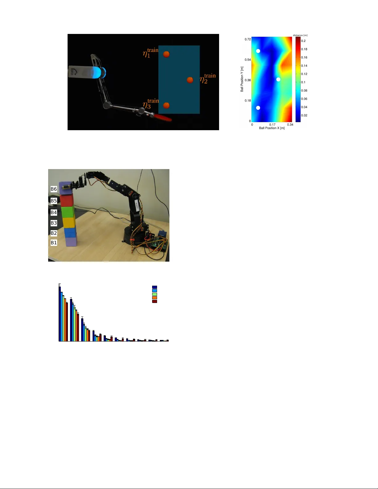
Multi-T ask P olicy Sear ch Marc Peter Deisenroth 1 , 2 , Peter Englert 3 , Jan Peters 2 , 4 , and Dieter Fox 5 Abstract — Learning policies that generalize across multiple tasks is an important and challenging resear ch topic in rein- for cement learning and robotics. T raining individual policies for every single potential task is often impractical, especially for continuous task variations, requiring more principled ap- proaches to share and transfer knowledge among similar tasks. W e present a novel approach for learning a nonlinear feedback policy that generalizes across multiple tasks. The key idea is to define a parametrized policy as a function of both the state and the task, which allows learning a single policy that generalizes across multiple known and unknown tasks. Applications of our novel approach to reinf orcement and imitation learning in real- robot experiments are shown. I . I N T RO D U C T I O N Complex robots often violate common modeling assump- tions, such as rigid-body dynamics. A typical example is a tendon-dri ven robot arm, shown in Fig. 1, for which these typical assumption are violated due to elasticities and springs. Therefore, learning controllers is a viable alternative to programming robots. T o learn controllers for complex robots, reinforcement learning (RL) is promising due to the generality of the RL paradigm [29]. Howe ver , without a good initialization (e.g., by human demonstrations [26], [3]) or specific expert knowledge [4] RL often relies on data- intensiv e learning methods (e.g., Q-learning). For a fragile robotic system, ho wev er, thousands of physical interactions are practically infeasible because of time-consuming exper- iments as well as the wear and tear of the robot. T o make RL practically feasible in robotics, we need to speed up learning by reducing the number of necessary interactions, i.e., robot experiments. For this purpose, model- based RL is often more promising than model-free RL, such as Q-learning or TD-learning [5]. In model-based RL, data is used to learn a model of the system. This model is then used for policy ev aluation and improvement, reducing the interaction time with the system. Howe ver , model-based RL suffers from model err ors as it typically assumes that the learned model closely resembles the true underlying dynamics [27], [26]. These model errors propagate through to the learned policy , whose quality inherently depends on the A concise version of this paper has been published at the IEEE Interna- tional Conference on Robotics and Automation (ICRA) 2014 [10]. The research leading to these results has received funding from the European Community’ s Seventh Framework Programme (FP7/2007-2013) under grant agreement #270327, ONR MURI grant N00014-09-1-1052, and the Department of Computing, Imperial College London. 1 Department of Computing, Imperial College London, UK 2 Department of Computer Science, TU Darmstadt, Germany 3 Department of Computer Science, Uni versity of Stuttgart, Germany 4 Max Planck Institute for Intelligent Systems, Germany 5 Department of Computer Science and Engineering, Uni versity of W ash- ington, W A, USA Fig. 1. T endon-driv en BioRob X4. quality of the learned model. A principled way of accounting for model errors and the resulting optimization bias is to take the uncertainty about the learned model into account for long-term predictions and policy learning [27], [6], [4], [18], [13]. Besides sample-efficient learning for a single task, generalizing learned concepts to new situations is a key research topic in RL. Learned controllers often deal with a single situation/context, e.g., they drive the system to a desired state. In a robotics conte xt, solutions for multiple related tasks are often desired, e.g., for grasping multiple objects [21] or in robot g ames, such as learning hitting mov ements in table tennis [22], or in generalizing kicking mov ements in robot soccer [7]. Unlike most other multi-task scenarios, we consider a set- up with a continuous set of tasks η . The objectiv e is to learn a policy that is capable of solving related tasks in the prescribed class. Since it is often impossible to learn individual policies for all conceiv able tasks, a multi-task learning approach is required that can generalize across these tasks. W e assume that during training , i.e., policy learning, the robot is given a small set of training tasks η train i . In the test phase , the learned policy is expected to generalize from the training tasks to previously unseen, but related, test tasks η test i . T w o general approaches exist to tackle this challenge by either hierarchically combining local controllers or a richer policy parametrization. First, local policies can be learned, and, subsequently , generalization can be achiev ed by combining them, e.g., by means of a gating network [17]. This approach has been successfully applied in RL [30] and robotics [22]. In [22] a gating network is used to generalize a set of motor primitives for hitting mov ements in robot-table tennis. The limitation of this approach is that it can only deal with conv ex combinations of local policies, implicitly requiring local policies that are linear in the policy parameters. 1 In [31], [7], it was proposed to share state-action 1 One way of making hierarchical models more flexible is to learn the hierarchy jointly with the local controllers. T o the best of our knowledge, such a solution does not exist yet. values across tasks to transfer kno wledge. This approach was successfully applied to kicking a ball with a NA O robot in the context of RoboCup. Howe ver , a mapping from source to target tasks is explicitly required. In [8], it is proposed to sample a number of tasks from a task distribution, learn the corresponding individual policies, and generalize them to new problems by combining classifiers and nonlinear regres- sion. In [19], [8] it is proposed to learn mappings from tasks to meta-parameters of a policy to generalize across tasks. The task-specific policies are trained independently , and the elementary movements are given by Dynamic Movement Primitiv es [16]. Second, instead of learning local policies one can parametrize the policy directly by the task. For instance, in [20], a value function-based transfer learning approach is proposed that generalizes across tasks by finding a regression function mapping a task-augmented state space to expected returns. W e follo w this second approach since it allows for generalizing nonlinear policies: During training, access to a set of tasks is giv en and a single controller is learned jointly for all tasks using policy search. Generalization to unseen tasks in the same domain is achiev ed by defining the policy as a function of both the state and the task. At test time, this allows for generalization to unseen tasks without retraining, which often cannot be done in real time. For learning the parameters of the multi-task policy , we use the P I L C O pol- icy search framework [11]. P I L C O learns flexible Gaussian process (GP) forward models and uses fast deterministic approximate inference for long-term predictions to achiev e data-efficient learning. In a robotics context, policy search methods have been successfully applied to many tasks [12] and seem to be more promising than value function-based methods for learning policies. Hence, this paper addresses two key problems in robotics: multi-task and data-ef ficient policy learning. I I . P O L I C Y S E A R C H F O R L E A R N I N G M U L T I P L E T AS K S W e consider dynamical systems x t +1 = f ( x t , u t ) + w with continuous states x ∈ R D and controls u ∈ R F and unknown transition dynamics f . The term w ∼ N ( 0 , Σ w ) is zero-mean i.i.d. Gaussian noise with cov ariance matrix Σ w . In (single-task) policy search, our objectiv e is to find a deterministic policy π : x 7→ π ( x , θ ) = u that minimizes the expected long-term cost J π ( θ ) = X T t =1 E x t [ c ( x t )] , p ( x 0 ) = N ( µ x 0 , Σ x 0 ) , (1) of following π for T steps. Note that the trajectory x 1 , . . . , x T depends on the policy π and, thus, the parameters θ . In Eq. (1), c ( x t ) is a given cost function of state x at time t . The policy π is parametrized by θ ∈ R P . T ypically , the cost function c incorporates some information about a task η , e.g., a desired target location x target or a trajectory . Finding a policy that minimizes Eq. (1) solves the task η of controlling the robot toward the target. A. T ask-Dependent P olicies W e propose to learn a single policy for all tasks jointly to generalize classical policy search to a multi-task scenario. W e −1.5 −1 −0.5 0 0.5 1 1.5 −9 −8.5 −8 −7.5 −7 −6.5 −6 Task η Control u Fig. 2. Generalization ability of a multi-task policy for the cart-pole experiment in Sec. III-A. Here, the state is fixed, the change in the controls is solely due to the change in the task. The black line represents the corresponding policy that has been augmented with the task. The controls of the training tasks are denoted by the red circles. The policy smoothly generalizes across test tasks. assume that the dynamics are stationary with the transition probabilities and control spaces shared by all tasks. By learning a single policy that is suf ficiently flexible to learn the training tasks η train i , we aim to obtain good generalization performance to related test tasks η test j by reducing the danger of ov erfitting to the training tasks, a common problem with current hierarchical approaches. T o learn a single controller for multiple tasks η k , we propose to make the policy a function of the state x , the parameters θ , and the task η , such that u = π ( x , η , θ ) . In this way , a trained policy has the potential to generalize to previously unseen tasks by computing different control signals for a fixed state x and parameters θ but varying tasks η k . Fig. 2 gives an intuition of what kind of generalization power we can expect from a polic y that uses state-task pairs as inputs: Assume a given policy parametrization, a fixed state, and fi ve training targets η train i . For each pair ( x , η train i , θ ) , the policy determines the corresponding con- trols π ( x , η train i , θ ) , which are denoted by the red circles. The dif ferences in these control signals are achie ved solely by changing η train i in π ( x , η train i , θ ) as x and θ were assumed fixed. The parametrization of the policy by θ and η implicitly determines the generalization power of π to new (but related) tasks η test j at test time. The policy for a fixed state b ut varying test tasks η test j is represented by the black curve. T o find good parameters of the multi-task policy , we incorporate our multi-task learning approach into the model-based P I L C O policy search framework [13]. The high-level steps of the resulting algorithm are summarized in Fig. 3. W e assume that a set of training tasks η train i is given. The parametrized policy π is initialized randomly , and, subsequently , applied to the robot, see line 1 in Fig. 3. Based on the initial collected data, a probabilistic GP forw ard model of the underlying robot dynamics is learned (line 3) to consistently account for model errors [25]. W e define the policy π as an explicit function of both the state x and the task η , which essentially means that the policy depends on a task-augmented state and u = π ( x , η , θ ) . Before going into detail, let us consider the case where a function g relates state and task. In this paper, we consider two cases: (a) A linear relationship between Fig. 3. Multi-T ask Policy Search 1: init: Pass in training tasks η train i , initialize policy pa- rameters θ randomly . Apply random control signals and record data. 2: r epeat 3: Update GP forward dynamics model using all data 4: repeat 5: Long-term predictions: Compute E η [ J π ( θ , η )] 6: Analytically compute gradient E η [ dJ π ( θ , η ) /d θ ] 7: Update policy parameters θ (e.g., BFGS) 8: until con vergence; return θ ∗ 9: Set π ∗ ← π ( θ ∗ ) 10: Apply π ∗ to robot and record data 11: until ∀ i : task η train i learned 12: Apply π ∗ to test tasks η test j the task η and the state x t with g ( x t , η ) = η − x t . For example, the state and the task (corresponding to a target location) can be both defined in camera coordinates, and the target location parametrizes and defines the task. (b) The task v ariable η and the state vector are not directly related, in which case g ( x t , η ) = η . For instance, the task variable could simply be an index. W e approximate the joint distribution p ( x t , g ( x t , η )) by a Gaussian N  µ x t µ η t  ,  Σ x t C xη t C η x t Σ η t  = : N  x x,η t | µ x,η t , Σ x,η t  , (2) where the state distribution is N  x t | µ x t , Σ x t  and C xη t is the cross-cov ariance between the state and g ( x t , η ) . The cross- cov ariances for g ( x t , η ) = η − x t are C xη t = − Σ x t . If the state and the task are not directly related, i.e., g ( x t , η ) = η , then C xη t = 0 . The Gaussian approximation of the joint distribution p ( x t , g ( x t , η )) in Eq. (2) serves as the input distribution to the controller function π . Although we assume that the tasks η test i are giv en deterministically at test time, introducing a task uncertainty Σ η t > 0 during training can make sense for two reasons: First, during training Σ η t defines a task distribution , which may allow for better generalization performance compared to Σ η t = 0 . Second, Σ η t > 0 induces uncertainty into planning and policy learning. Therefore, Σ η t serves as a regularizer and makes policy ov erfitting less likely . B. Multi-T ask P olicy Evaluation For policy ev aluation, we analytically approximate the expected long-term cost J π ( θ ) by av eraging over all tasks η , see line 5 in Fig. 3, according to E η [ J π ( θ , η )] ≈ 1 M X M i =1 J π ( θ , η train i ) , (3) where M is the number of tasks considered during training. The expected cost J π ( θ , η train i ) corresponds to Eq. (1) for a specific training task η train i . The intuition behind the expected long-term cost in Eq. (3) is to allow for learning a single controller for multiple tasks jointly . Hence, the controller parameters θ have to be updated in the context of all tasks. The resulting controller is not necessarily optimal for a sin- gle task, but (neglecting approximations and local minima) optimal across all tasks on average, presumably leading to good generalization performance. The expected long-term cost J π ( θ , η train i ) in Eq. (3) is computed as follows. First, based on the learned GP dynamics model, ap- proximations to the long-term predictiv e state distributions p ( x 1 | η ) , . . . , p ( x T | η ) are computed analytically: Giv en a joint Gaussian prior distribution p ( x t , u t | η ) , the distribution of the successor state p ( x t +1 | η train i ) = Z Z Z p ( x t +1 | x t , u t ) p ( x t , u t | η train i ) d f d x t d u t (4) cannot be computed analytically for nonlinear covari- ance functions. Howe ver , we approximate it by a Gaus- sian distribution N  x t +1 | µ x t +1 , Σ x t +1  using exact moment matching [24], [11]. In Eq. (4), the transition probability p ( x t +1 | x t , u t ) = p ( f ( x t , u t ) | x t , u t ) is the GP predic- tiv e distribution at ( x t , u t ) . Iterating the moment-matching approximation of Eq. (4) for all time steps of the finite horizon T yields Gaussian marginal predictiv e distributions p ( x 1 | η train i ) , . . . , p ( x T | η train i ) . Second, these approximate Gaussian long-term pre- dictiv e state distrib utions allow for the computation of the expected immediate cost E x t [ c ( x t ) | η train i ] = R c η ( x t ) p ( x t | η train i ) d x t for a particular task η train i , where p ( x t | η train i ) = N  x t | µ x t , Σ x t  and c η is a task-specific cost function. This integral can be solved analytically for many choices of the immediate cost function c η , such as polyno- mials, trigonometric functions, or unnormalized Gaussians. Summing the values E x t [ c ( x t ) | η train i ] from t = 1 , . . . , T finally yields J π ( θ , η train i ) in Eq. (3). C. Gr adient-based P olicy Impr ovement The deterministic and analytic approximation of J π ( θ , η ) by means of moment matching allows for an analytic com- putation of the corresponding gradient dJ π ( θ , η ) /d θ with respect to the policy parameters θ , see Eq. (3) and line 6 in Fig. 3, which are given by dJ π ( θ , η ) d θ = X T t =1 d d θ E x t [ c ( x t ) | η ] . (5) These gradients can be used in any gradient-based optimiza- tion toolbox, e.g., BFGS (line 7). Analytic computation of J π ( θ , η ) and its gradients dJ π ( θ , η ) /d θ is more efficient than estimating policy gradients through sampling: For the latter , the variance in the gradient estimate grows quickly with the number of polic y parameters and the horizon T [23]. Computing the deriv ativ es of J π ( θ , η train i ) with respect to the policy parameters θ requires repeated application of the chain-rule. Defining E t : = E x t [ c ( x t ) | η train i ] in Eq. (5) yields d E t d θ = d E t dp ( x t ) dp ( x t ) d θ : = ∂ E t ∂ µ x t d µ x t d θ + ∂ E t ∂ Σ x t d Σ x t d θ , (6) where we took the deriv ativ e with respect to p ( x t ) , i.e., the parameters of the state distribution p ( x t ) . In Eq. (6), this amounts to computing the deriv ativ es of E t with respect to the mean µ x t and cov ariance Σ x t of the Gaussian approxi- mation of p ( x t ) . The chain-rule yields the total deriv ative of p ( x t ) with respect to θ dp ( x t ) d θ = ∂ p ( x t ) ∂ p ( x t − 1 ) dp ( x t − 1 ) d θ + ∂ p ( x t ) ∂ θ . (7) In Eq. (7), we assume that the total deriv ative dp ( x t − 1 ) /d θ is known from the computation for the previous time step. Hence, we only need to compute the partial deriv ativ e ∂ p ( x t ) /∂ θ . Note that x t = f ( x t − 1 , u t − 1 ) + w and u t − 1 = π ( x t − 1 , g ( x t − 1 , η ) , θ ) . Therefore, we obtain, with the Gaus- sian approximation to the marginal state distribution p ( x t ) , ∂ p ( x t ) /∂ θ = { ∂ µ x t /∂ θ , ∂ Σ x t /∂ θ } with ∂ { µ x t , Σ x t } ∂ θ = ∂ { µ x t , Σ x t } ∂ p ( u t − 1 ) ∂ p ( u t − 1 ) ∂ θ = ∂ { µ x t , Σ x t } ∂ µ u t − 1 ∂ µ u t − 1 ∂ θ + ∂ { µ x t , Σ x t } ∂ Σ u t − 1 ∂ Σ u t − 1 ∂ θ . (8) Here, the distribution p ( u t − 1 ) = Z π ( x t − 1 , g ( x t − 1 , η ) , θ ) p ( x t − 1 ) d x t − 1 of the control signal is approximated by a Gaussian with mean µ u t − 1 and covariance Σ u t − 1 . These moments (and their gradients with respect to θ ) can often be computed analyt- ically , e.g., in linear models with polynomial or Gaussian basis functions. The augmentation of the policy with the (transformed) task variable requires an additional layer of gradients for computing dJ π ( θ ) /d θ . The variable transfor- mation affects the partial deri vati ves of µ u t − 1 and Σ u t − 1 (marked red in Eq. (8)), such that ∂ { µ u t − 1 , Σ u t − 1 } ∂ { µ x t − 1 , Σ x t − 1 , θ } = ∂ { µ u t − 1 , Σ u t − 1 } ∂ p ( x t − 1 , g ( x t − 1 , η )) × ∂ p ( x t − 1 , g ( x t − 1 , η )) ∂ { µ x t − 1 , Σ x t − 1 , θ } , (9) which can often be computed analytically . Similar to [11], we combine these deri vati ves with the gradients in Eq. (8) via the chain and product-rules, yielding an analytic gradient dJ π ( θ , η train i ) /d θ in Eq. (3), which is used for gradient-based policy updates, see lines 6 – 7 in Fig. 3. I I I . E V A L UAT I ON S A N D R E S U LT S In the following, we analyze our approach to multi-task policy search on three scenarios: 1) the under-actuated cart- pole swing-up benchmark, 2) a lo w-cost robotic manipulator system that learns block stacking, and 3) an imitation learn- ing ball-hitting task with a tendon-driven robot. In all cases, the system dynamics were unkno wn and inferred from data using GPs. A. Multi-T ask Cart-P ole Swing-up W e applied our proposed multi-task policy search to learning a model and a controller for the cart-pole swing- up. The system consists of a cart with mass 0 . 5 kg and a pendulum of length 0 . 6 m and mass 0 . 5 kg attached to the cart. Every 0 . 1 s , an external force was applied to the cart, but not to the pendulum. The friction between cart and ground was 0 . 1 Ns / m . The state x = [ χ, ˙ χ, ϕ, ˙ ϕ ] of the system comprised the position χ of the cart, the v elocity ˙ χ of the cart, the angle ϕ of the pendulum, and the angular velocity ˙ ϕ of the pendulum. For the equations of motion, we refer to [9]. The nonlinear controller was parametrized as a regularized RBF network with 100 Gaussian basis functions. The controller parameters were the locations of the basis functions, a shared (diagonal) width-matrix, and the weights, resulting in approximately 800 policy parameters. Initially , the system was expected to be in a state, where the pendulum hangs down; more specifically , p ( x 0 ) = N ( 0 , 0 . 1 2 I ) . By pushing the cart to the left and to the right, the objecti ve was to swing the pendulum up and to balance it in the inv erted position at a target location η of the cart specified at test time , such that x target = [ η , ∗ , π + 2 kπ , ∗ ] with η ∈ [ − 1 . 5 , 1 . 5] m and k ∈ Z . The cost function c in Eq. (1) was chosen as c ( x ) = 1 − exp( − 8 k x − x target k 2 ) ∈ [0 , 1] and penalized the Euclidean distance of the tip of the pendulum from its desired in verted position with the cart being at target location η . Optimally solving the task required the cart to stop at the target location η . Balancing the pendulum with the cart offset by 20 cm caused an immediate cost (per time step) of about 0.4. W e considered four experimental setups: Nearest neighbor independent controllers (NN-IC): Nearest-neighbor baseline experiment with fiv e indepen- dently learned controllers for the desired swing-up locations η = {± 1 m , ± 0 . 5 m , 0 m } . Each controller was learned using the P I L C O framew ork [13] in 10 trials with a total experience of 200 s . For the test tasks η test , we applied the controller with the closest training task η train . Re-weighted independent controllers (RW -IC): Training was identical to NN-IC. At test time, we combined indi vidual controllers using a gating network, similar to [22], resulting in a conv ex combination of local policies. The gating- network weights were v i = exp  − 1 2 κ k η test − η train i k 2  P | η train | j exp  − 1 2 κ k η test − η train j k 2  , (10) such that the applied control signal was u = P i v i π i ( x ) . An extensiv e grid search resulted in κ = 0 . 0068 m 2 , leading to the best test performance in this scenario, making R W -IC nearly identical to the NN-IC. Multi-task policy search, Σ η = 0 (MTPS0): Multi-task policy search with five kno wn tasks during training, which only dif fer in the location of the cart where the pendulum is supposed to be balanced. The target locations were η train = {± 1 m , ± 0 . 5 m , 0 m } . Moreov er , g ( x t , η ) = η − χ ( t ) and Σ η = 0 . W e sho w results after 20 trials, i.e., a total experience of 70 s only . Multi-task policy search, Σ η > 0 (MTPS+): Multi- task policy search with the fiv e training tasks η train = {± 1 m , ± 0 . 5 m , 0 m } , but with training task co variance Σ η = diag([0 . 1 2 , 0 , 0 , 0]) . W e show results after 20 trials, i.e., 70 s total experience. For testing the performance of the algorithms, we applied the learned policies 100 times to the test-tar get locations η test = − 1 . 5 , − 1 . 4 , . . . , 1 . 5 . Every time, the initial state of a rollout was sampled from p ( x 0 ) . For the MTPS experiments, we plugged the test tasks into Eq. (2) to compute the corresponding control signals. Fig. 4 illustrates the generalization performance of the learned controllers. The horizontal axes denote the locations η test of the target position of the cart at test time. The height of the bars show the a verage (over trials) cost per time step. The means of the training tasks η train are the location of the red bars. For Experiment 1, Fig. 4(d) sho ws the distribution p ( η train i ) used during training as the bell-curves, which approximately covers the range η ∈ [ − 1 . 2 m , 1 . 2 m] . The NN-IC controller in the nearest-neighbor baseline, see Fig. 4(a), balanced the pendulum at a cart location that was not further away than 0 . 2 m , which incurred a cost of up to 0.45. In Fig. 4(b), the performances for the hierarchical R W - IC controller are shown. The performance for the best value κ in the gating network, see Eq. (10), was similar to the performance of the NN-IC controller . Howe ver , between the training tasks for the local controllers, where the test tasks were in the range of [ − 0 . 9 m , 0 . 9 m] , the con ve x combination of local controllers led to more failures than in NN-IC, where the pendulum could not be swung up successfully: Con- ve x combinations of nonlinear local controllers ev entually decreased the (non-existing) generalization performance of R W -IC. Fig. 4(c) shows the performance of the MTPS0 controller . The MTPS0 controller successfully performed the swing-up plus balancing task for all tasks η test close to the training tasks. Howe ver , the performance varied relatively strongly . Fig. 4(d) sho ws that the MTPS+ controller successfully performed the swing-up plus balancing task for all tasks η test at test time that were suf ficiently cov ered by the uncertain training tasks η train i , i = 1 , . . . , 5 , indicated by the bell curves representing Σ η > 0 . Relatively constant performance across the test tasks co vered by the bell curves was achie ved. An average cost of 0.3 meant that the pendulum might be balanced with the cart slightly offset. Fig. 2 shows the learned MTPS+ policy for all test tasks η test with the state x = µ 0 fixed. T ab . I summarizes the expected costs across all test tasks η test . W e av eraged over all test tasks and 100 applications of the learned policy , where the initial state was sampled from p ( x 0 ) . Although NN-IC and R W -IC performed swing- up reliably , they incurred the largest cost: For most test tasks, they balanced the pendulum at the wrong cart position as they could not generalize from training tasks to unseen test tasks. In the MTPS experiments, the av erage cost was lowest, indicating that our multi-task policy search approach T ABLE I M U L T I - T A S K C A RT - P O LE S W IN G - U P : A V E R AG E C O ST S AC RO S S 3 1 T ES T TAS K S η T ES T . NN-IC RW -IC MTPS0 MTPS+ Cost 0.39 0.4 0.33 0.30 −1.5 −1 −0.5 0 0.5 1 1.5 −9.5 −9 −8.5 −8 −7.5 −7 −6.5 −6 Task η Control u Policy augmentation Hierarchical policy Fig. 5. T wo multi-task policies for a given state x , but v arying task η . The black policy is obtained by applying our proposed multi-task approach (MTPS+); the blue, dashed policy is obtained by hierarchically combining local controllers (R W -IC). The training tasks are η = {± 1 , ± 0 . 5 , 0 } . The corresponding controls u = π ( x , η ) are marked by the red circles (MTPS+) and the green stars (RW -IC), respectiv ely . MTPS+ generalizes more smoothly across tasks, whereas the hierarchical combination of inde- pendently trained local policies does not generalize well. is beneficial. MTPS+ led to the best overall generalization performance, although it might not solve each individual test task optimally . Fig. 5 illustrates the difference in generalization per- formance between our MTPS+ approach and the R W -IC approach, where controls u i from local policies π i are combined by means of a gating netw ork. Since the local policies are trained independently , a (conv ex) combination of local controls makes only sense in special cases, e.g., when the local policies are linear in the parameters. In this example, howe ver , the local policies are nonlinear . Since the local policies are learned independently , their overall gener- alization performance is poor . On the other hand, MTPS+ learns a single policy for a task η i always in the light of all other tasks η j 6 = i as well, and, therefore, leads to an overall smooth generalization. B. Multi-T ask Robot Manipulator Our proposed multi-task learning method has been ap- plied to a block-stacking task using a low-cost, off-the-shelf robotic manipulator ($370) by L ynxmotion [1], see Fig. 6(a), and a PrimeSense [2] depth camera ($130) used as a visual sensor . The arm had six controllable degrees of freedom: base rotate, three joints, wrist rotate, and a gripper (open/ close). The plastic arm could be controlled by commanding both a desired configuration of the six servos (via their pulse durations) and the duration for executing the command [14]. The camera was identical to the Kinect sensor , providing a synchronized depth image and a 640 × 480 RGB image at 30 Hz . W e used the camera for 3D-tracking of the block in the robot’ s gripper . The goal was to make the robot learn to stack a tower of six blocks using multi-task learning. The cost function c in Eq. (1) penalized the distance of the block in the gripper from the desired drop-off location. W e only specified the 3D camera coordinates of the blocks B2, B4, and B5 as the training tasks η train , see Fig. 6(a). Thus, at test time, stacking B3 and B6 required exploiting the generalization of −1.5 −1 −0.5 0 0.5 1 1.5 0 0.1 0.2 0.3 0.4 0.5 0.6 0.7 0.8 0.9 1 target location (test time) per−step cost (a) NN-IC: No generalization. −1.5 −1 −0.5 0 0.5 1 1.5 0 0.1 0.2 0.3 0.4 0.5 0.6 0.7 0.8 0.9 1 target location (test time) per−step cost (b) R W -IC: No generalization. −1.5 −1 −0.5 0 0.5 1 1.5 0 0.1 0.2 0.3 0.4 0.5 0.6 0.7 0.8 0.9 1 target location (test time) per−step cost (c) MTPS0: Some generalization. −1.5 −1 −0.5 0 0.5 1 1.5 0 0.1 0.2 0.3 0.4 0.5 0.6 0.7 0.8 0.9 1 target location (test time) per−step cost (d) MTPS+: Good generalization in the “coverage” of the Gaussians. Fig. 4. Generalization performance for the multi-task cart-pole swing-up. The graphs show the expected cost per time step along with twice the standard errors. the multi-task policy search. W e chose g ( x , η ) = η − x . Moreov er , we set Σ η such that the task space, i.e., all 6 blocks, was well covered. The mean µ 0 of the initial distribution p ( x 0 ) corresponded to an upright configuration of the arm. A GP dynamics model was learned that mapped the 3D camera coordinates of the block in the gripper and the commanded controls at time t to the corresponding 3D coordinates of the block in the gripper at time t + 1 , where the control signals were changed at a rate of 2 Hz . Note that the learned model is not an inv erse kinematics model as the robot’ s joint state is unknown. W e used an affine policy u t = π ( x t , η , θ ) = Ax x,η t + b , where θ = { A , b } . The policy now defined a mapping π : R 6 → R 4 , where the four controlled degrees of freedom were the base rotate and three joints. W e report results based on 16 training trials, each of length 5 s , which amounts to a total experience of 80 s only . The test phase consisted of 10 trials per stacking task, where the arm was supposed to stack the block on the currently topmost block. The tasks η test j at test time corresponded to stacking blocks B2–B6 in Fig. 6(a). Fig. 6(b) sho ws the av erage distance of the block in the gripper from the target position, which was b = 4 . 3 cm abov e the topmost block. Here, “block2” means that the task was to mo ve block B2 in the gripper on top of block 1. The horizontal axis sho ws times at which the manipulator’ s control signal was changed (rate 2 Hz ), the vertical axis shows the average distances (over 10 test trials) to the target position in meters. For all blocks (including blocks B3 and B6, which were not part of the training tasks η train ) the distances approached zero over time. Thus, the learned multi-task controller was able to interpolate (block B3) and extrapolate (block B6) from the training tasks to the test tasks without re-training. C. Multi-T ask Imitation Learning of Ball-Hitting Movements W e demonstrate that our MTPS approach can also be ap- plied to imitation learning. Instead of defining a cost function c in Eq. (1), a teacher provides demonstrations that the robot should imitate. W e show that our MTPS approach allows to generalize from demonstrated beha vior to beha viors that ha ve not been observed before. In [15], we dev eloped a method for model-based imitation learning based on probabilistic trajectory matching for a single task. The ke y idea is to match a distrib ution ov er predicted robot trajectories p ( τ π ) directly (a) Set-up for the imitation learning experiments. The orange balls represent the three training tasks η train i . The blue rectangle indicates the regions of the test tasks η test j for our learned controller to which we want to generalize. distanc e [m] (b) The white discs are the train- ing task locations. Blue and cyan indicate that the task was solved successfully . Fig. 7. Set-up and results for the imitation learning experiments with a bio-inspired BioRob TM . B1 B2 B3 B4 B5 B6 (a) Low-cost manipulator by L ynxmotion [1] performing a block-stacking task. 0.5 1 1.5 2 2.5 3 3.5 4 4.5 5 0 0.1 0.2 0.3 0.4 0.5 time in seconds average distance to target in meters block2 block3 block4 block5 block6 (b) A verage distances of the block in the gripper from the target position (with twice the standard error). Fig. 6. Experimental setup and results for the multi-task block-stacking task. A controller was learned directly in the task space using visual feedback from a PrimeSense depth camera. with an observed distribution p ( τ exp ) ov er expert trajectories τ exp by finding a policy π ∗ that minimizes the KL di ver gence [28] between them. In this paper, we extend this imitation learning approach to a multi-task scenario to jointly learning to imitate multiple tasks from a small set of demonstrations. In particular , we applied our multi-task learning approach to learning a con- troller for hitting movements with variable ball positions in a 2D-plane using the tendon-driv en BioRob TM X4, a five DoF compliant, light-weight robotic arm, capable of achieving high accelerations, see Fig. 7(a). The torques are transferred from the motor to the joints via a system of pulleys, driv e cables, and springs, which, in the biomechanically-inspired context, represent tendons and their elasticity . While the BioRob’ s design has advantages ov er traditional approaches, modeling and controlling such a compliant system is chal- lenging. In our imitation-learning experiment, we considered three joints of the robot, such that the state x ∈ R 6 contained the joint positions q and velocities ˙ q of the robot. The controls u ∈ R 3 were giv en by the corresponding motor torques, directly determined by the policy π . F or learning a controller, we used an RBF network with 250 Gaussian basis functions, where the policy parameters comprised the locations of the basis functions, their weights, and a shared diagonal cov ariance matrix, resulting in about 2300 policy parameters. Policy learning required about 20 minutes computation time. Unlike in the previous examples, we represented a task as a two-dimensional vector η ∈ R 2 corresponding to the ball position in Cartesian coordinates in an arbitrary reference frame within the hitting plane. As the task representation η was basically an index and, hence, unrelated to the state of the robot, g ( x , η ) = η , and the cross-cov ariances C xη in Eq. (2) were 0 . As training tasks η train j , we defined hitting movements for three different ball positions, see Fig. 7(a). For each training task, an expert demonstrated two hitting movements via kinesthetic teaching. Our goal w as to learn a single polic y that a) learns to imitate three distinct expert demonstrations, and b) generalizes from demonstrated behaviors to tasks that were not demonstrated. In particular, these tests tasks were defined as hitting balls in a larger region around the training locations, indicated by the blue box in Fig. 7(a). W e set the matrices Σ η such that the blue box was cov ered well. Fig. 7(b) shows the performance results as a heatmap after 15 iterations of Alg. 3. The ev aluation measure was the distance in m between the ball position and the center of the table-tennis racket. W e computed this error in a regular 7x5 grid of the blue area in Fig. 7(a). The distances in the blue and cyan areas were sufficient to successfully hit the ball (the racket’ s radius is about 0 . 08 m ). Hence, our approach successfully generalized from given demonstrations to new tasks that were not in the library of demonstrations. D. Remarks Controlling the cart-pole system to dif ferent target location is a task that could be solved without the task-augmentation of the controller inputs: It is possible to learn a controller that depends only on the position of the cart relative to the target location—the control signals should be identical when the cart is at location χ , the target location is at χ + ε or when the cart is at location at position x 2 , and the target location is at x 2 + ε . Our approach, howe ver , learns these in variances automatically , i.e., it does not require an intricate knowledge of the system/controller properties. Note that a linear combination of local controllers usually does not lead to success in the cart-pole system, which requires a nonlinear controller for the joint task of swinging up the pendulum and balancing it in the inv erted position. In the case of the L ynx-arm, these in variances no longer exist as the optimal control signal depends on the absolute position of the arm, not only on the relativ e distance to the target. Since a linear controller is sufficient to learn block stacking, a con vex combination of indi vidual controllers should be able to generalize from the trained blocks to new targets if no extrapolation is required. I V . C O N C L U S I O N A N D F U T U R E W O R K W e have presented a policy-search approach to multi-task learning for robots, where we assume stationary dynamics. Instead of combining local policies using a gating network, which only works for linear-in-the-parameters policies, our approach learns a single policy jointly for all tasks. The key idea is to explicitly parametrize the policy by the task and, therefore, enable the policy to generalize from training tasks to similar , b ut unknown, tasks at test time. This generalization is phrased as an optimization problem, jointly with learning the policy parameters. For solving this optimization problem, we incorporated our approach into the P I L C O policy search framew ork, which allo ws for data- efficient policy learning. W e hav e reported promising results on multi-task RL on a standard benchmark problem and on a robotic manipulator . Our approach also applies to imitation learning and generalizes imitated behavior to solving tasks that were not in the library of demonstrations. In this paper , we considered the case that re-training the policy after a test run is not allo wed. Relaxing this constraint and incorporating the experience from the test trials into a subsequent iteration of the learning procedure would impro ve the av erage quality of the controller . In future, we will jointly learn the task representation for the policy and the policy parametrization. Thereby , it will not be necessary to specify any interdependence between task and state space a priori, but this interdependence will be learned from data. R E F E R E N C E S [1] http://www .lynxmotion.com. [2] http://www .primesense.com. [3] P . Abbeel and A. Y . Ng. Exploration and Apprenticeship Learning in Reinforcement Learning. In ICML , 2005. [4] P . Abbeel, M. Quigley , and A. Y . Ng. Using Inaccurate Models in Reinforcement Learning. In ICML , 2006. [5] C. G. Atkeson and J. C. Santamar ´ ıa. A Comparison of Direct and Model-Based Reinforcement Learning. In ICRA , 1997. [6] J. A. Bagnell and J. G. Schneider . Autonomous Helicopter Control using Reinforcement Learning Policy Search Methods. In ICRA , 2001. [7] S. Barrett, M. E. T aylor , and P . Stone. T ransfer Learning for Reinforcement Learning on a Physical Robot. In AAMAS , 2010. [8] B. C. da Silva, G. Konidaris, and A. G. Barto. Learning Parametrized Skills. In ICML , 2012. [9] M. P . Deisenroth. Efficient Reinforcement Learning using Gaussian Pr ocesses . KIT Scientific Publishing, 2010. ISBN 978-3-86644-569-7. [10] M. P . Deisenroth, P . Englert, J. Peters, and D. Fox. Multi-T ask Policy Search for Robotics. In ICRA , 2014. [11] M. P . Deisenroth, D. Fox, and C. E. Rasmussen. Gaussian Processes for Data-Efficient Learning in Robotics and Control. IEEE-TP AMI , 2014. [12] M. P . Deisenroth, G. Neumann, and J. Peters. A Survey on P olicy Sear ch for Robotics , v olume 2 of F oundations and T r ends in Robotics . NO W Publishers, 2013. [13] M. P . Deisenroth and C. E. Rasmussen. PILCO: A Model-Based and Data-Efficient Approach to Policy Search. In ICML , 2011. [14] M. P . Deisenroth, C. E. Rasmussen, and D. F ox. Learning to Control a Low-Cost Manipulator using Data-Efficient Reinforcement Learning. In RSS , 2011. [15] P . Englert, A. P araschos, J. Peters, and M. P . Deisenroth. Model-based Imitation Learning by Proabilistic Trajectory Matching. In ICRA , 2013. [16] A. J. Ijspeert, J. Nakanishi, and S. Schaal. Learning Attractor Landscapes for Learning Motor Primiti ves. In NIPS , 2002. [17] R. A. Jacobs, M. I. Jordan, S. J. Nowlan, and G. E. Hinton. Adaptive Mixtures of Local Experts. Neural Computation , 3:79–87, 1991. [18] J. K o, D. J. Klein, D. Fox, and D. Haehnel. Gaussian Processes and Reinforcement Learning for Identification and Control of an Autonomous Blimp. In ICRA , 2007. [19] J. Kober , A. W ilhelm, E. Oztop, and J. Peters. Reinforcement Learning to Adjust Parametrized Motor Primitives to New Situations. Autonomous Robots , 33(4):361–379, 2012. [20] G. Konidaris, I. Scheidwasser , and A. G. Barto. Transfer in Reinforce- ment Learning via Shared Features. JMLR , 13:1333–1371, 2012. [21] O. Kroemer, R. Detry , J. Piater , and J. Peters. Combining Activ e Learning and Reactive Control for Robot Grasping. Robotics and Autonomous Systems , 58:1105–1116, 2010. [22] K. M ¨ ulling, J. Kober , O. Kroemer, and J. Peters. Learning to Select and Generalize Striking Movements in Robot T able T ennis. IJRR , 2013. [23] J. Peters and S. Schaal. Policy Gradient Methods for Robotics. In IR OS , 2006. [24] J. Qui ˜ nonero-Candela, A. Girard, J. Larsen, and C. E. Rasmussen. Propagation of Uncertainty in Bayesian Kernel Models—Application to Multiple-Step Ahead Forecasting. In ICASSP , 2003. [25] C. E. Rasmussen and C. K. I. W illiams. Gaussian Pr ocesses for Machine Learning . The MIT Press, 2006. [26] S. Schaal. Learning From Demonstration. In NIPS . 1997. [27] J. G. Schneider . Exploiting Model Uncertainty Estimates for Safe Dynamic Control Learning. In NIPS . 1997. [28] K. Solomon. Information Theory and Statistics . W iley , New Y ork, 1959. [29] R. S. Sutton and A. G. Barto. Reinfor cement Learning: An Introduc- tion . The MIT Press, 1998. [30] M. E. T aylor and P . Stone. Cross-Domain Transfer for Reinforcement Learning. In ICML , 2007. [31] M. E. T aylor and P . Stone. T ransfer Learning for Reinforcement Learning Domains: A Survey . JMLR , 10(1):1633–1685, 2009.