Structured Priors for Sparse-Representation-Based Hyperspectral Image Classification

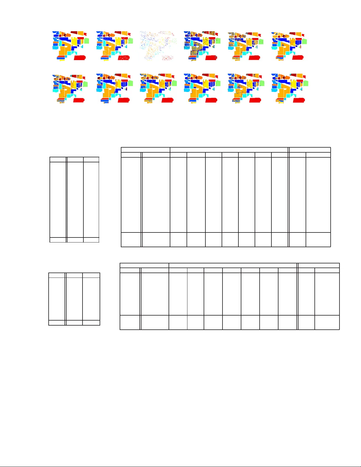
IEEE GEOSCIENCE AND REMOTE SENSI NG LET TER 1 Structured Priors for Sparse-Representat ion-Based Hyperspectral Image Classification Xiaoxia Sun, Qing Qu, Nasse r M. Nasrabadi, F ellow , IEEE, and Trac D. T ran, Senior Member , IEEE Abstract —Pixel-wise classification, where each pixel is assigned to a predefined class, is one of the most important procedures in hyperspectral image (HSI) analysis. By repr esenting a test pixel as a linear combination of a small subset of labeled pixels, a sparse repre sentation classifier (SRC) giv es rather plausible results compared wi th that of traditional classifiers such as the support vector machine (SVM). Recently , b y incorporating additional structured sparsity priors, the second generation SRCs hav e appeared in the literature and are reported to fu rther impro ve the perfo rmance of HSI. Th ese priors are b ased on exploiting the spatial d ependencies between the neighboring pixels, the inherent structure of the d ictionary , or both. In this p aper , we r eview and compare se veral structured p riors f or sparse- repre sentation-based HSI classifi cation. W e also p ropose a new structured prior called th e low rank group prior , which can be considered as a modification of the low rank p rior . Furthermore, we will inv estigate h ow di fferent structured priors i mpro ve th e result for the HSI classification. Index T erms —hyperspectral image, sparse representation, structured p riors, classification I . I N T R O D U C T I O N O NE of th e most imp ortant pro cedures in HSI is image classification, wh ere th e pixels are lab eled to on e of the classes based on the ir sp ectral characteristics. Due to th e n u- merous deman ds in min eralogy , agr iculture an d surveillance, the HSI classification task is developing very r apidly an d a large nu mber of techn iques h av e been pro posed to tackle this problem [1]. Com paring with previous app roaches, SVM is found h ighly effecti ve o n both co mputation al efficiency an d classification results. A wide variety o f SVM’ s modifications have been proposed to improve its perform ance. Some of them incorpo rate the co ntextual in formation in the classifiers [2], [3]. Others design sparse SVM in or der to pu rsue a sparse decision rule b y usin g ℓ 1 -norm as th e regularizer [4]. Recently , SRC has be en pr oposed to solve many co mputer vision tasks [5], [6], wh ere th e use o f spa rsity as a prior of ten leads to state-of- the-art p erform ance. SRC has also be en a p- plied to HSI classification [7], relying on the o bservation that hypersp ectral pixels belonging to th e s ame class approximately lie in the same low-dimensional subspace. In o rder to alleviate the p roblem in troduced b y the lac k of sufficient train ing data, Haq et a l . [8] pr oposed the ho motopy-ba sed SRC. Another way to solve the prob lem o f insufficient train ing data is to X.Sun, Q. Qu and T . D. Tran are with the Department of E lect rical and Computer Engineerin g, T he Johns Hopkins Uni versity , Baltimore, MD 21218 USA (e-mail: xsun9@jhu.edu; qqu2@jhu.edu; trac@jhu.edu). This work has been partia lly supported by NSF under Grants CCF-1117545, AR O under Grants 60219-MA, and ONR under grant N00014121076 5. N. M. Nasrabadi is with U.S. Army Research Laboratory , Adelphi, MD 20783 USA (e-mail: nnasraba@a rl.army .m il). employ the con textual in formation of n eighbor ing pixels in the classifier , such as spectral-spatial constraint classification [9]. In SRC, a test sample y ∈ R P , where P is the numb er of spectral band s, can be written as a sparse linear co mbination of all the tr aining pixels ( atoms in a dic tionary) as ˆ x = min x 1 2 k y − Ax k 2 2 + λ k x k 1 , (1) where x ∈ R N , k x k 1 = N P i =1 | x i | is ℓ 1 -norm . A = [ a 1 , a 2 , · · · , a N ] is a structured dictionar y for med fr om con - catenation of several class-wise sub-diction aries, { a i } i =1 ,...,N are the column s of A and N is the total n umber o f training samples from all th e K classes, an d λ is a scalar regularization parameter . The class lab el for the test pixel y is d etermined by the minimum residu al betwee n y and its app roximation from each class-wise sub -dictionar y: cl ass ( y ) = arg min g k y − A δ g ( x ) k 2 2 , (2) where g ⊂ { 1 , 2 , · · · , K } is the gro up or class in dex, and δ g ( x ) is the indicator o peration zeroing o ut all elements of x that do no t b elong to the class g . In the case of HSI, SRC alw a ys suffers from the no n- uniquen ess o r instability of the sparse coefficients due to the high mutual coherency of the d ictionary [10]. Fortunately , a better recon structed signal and a mor e robust representa- tion can be obtain ed by eithe r exploring the d ependen cies of n eighbor ing pixels or exploiting the inhe rent dictiona ry structure. Recently , struc tured prior s h a ve been inco rporated into HSI classification [ 7], which can be sorted into thre e categories. ( a ) Prio rs that only exploit the correlatio ns an d depend encies a mong th e n eighbo ring spectral p ixels or their sparse coefficient vecto rs, wh ich includes joint sparsity [1 2], graph regularized Lasso ( referred as the Lap lacian r egularized Lasso) [1 3] a nd th e low-rank Lasso [14]. ( b ) Priors that only exploit the inhere nt structure o f the dictio nary , such a s gr oup Lasso [15]. ( c ) Prior s that enforce structu ral informa tion o n both spar se coefficients and dictionar y , such as collabora - ti ve gro up Lasso [16] and collaborative hiera rchical Lasso (CHiLasso) [17]. Besides SRC, structur ed spar sity prior can also be incorp orated into other classifiers such a s the lo gistic regression classifiers [18]. The main contributions of this paper are (a) to assess th e SRC perf ormance u sing various stru ctured sparsity p riors for HSI classification, and (b) to prop ose a conceptua lly similar prior to CHiLasso, which is called the low-rank group prior . IEEE GEOSCIENCE AND REMOTE SENSI NG LET TER 2 This prior is based on the assumption that p ure or m ixed pixels from the same c lasses are hig hly corr elated and can be represented by a combin ation of sparse low-rank gro ups (classes). Th e prop osed p rior takes advantage of b oth the group sparsity prior, which enforces sparsity across the groups, and the low rank prior, wh ich enco urages sparsity within th e group s, b y o nly u sing on e regularizer . In the following sections, we in vestigate the roles o f dif- ferent structured priors imposed on the SRC optimization algorithm . Starting with the classical sparsity ℓ 1 -norm prior, we then introduc e several d ifferent prio rs with experim ental results. The structured prio rs discussed ar e joint sparsity , Laplacian spar sity , g roup sparsity , sparse grou p spar sity , low- rank and low-rank g roup pr ior . I I . H S I C L A S S I FI C A T I O N V I A D I FF E R E N T S T R U C T U R E D S PA R S E P R I O R S A. J oint S parsity Prior In HSI , pixels within a small neig hborh ood u sually co nsist of similar materials. Thus, their spectral charac teristics are highly cor related. The spatial co rrelation b etween neig hborin g pixels can be indirectly incorp orated thro ugh a join t sparsity model (JSM) [11] by assumin g that th e un derlying sparse vectors associated with th ese p ixels share a co mmon spar sity support. Consid er pixels in a small neighb orhoo d of T pixels. Let Y ∈ R P × T represent a ma trix wh ose column s correspon d to pixels in a spatial neighbo rhood in a hypersp ectral image. Columns of Y = [ y 1 , y 2 , · · · , y T ] can b e represented as a linear combin ation of d ictionary atoms Y = AX , where X = [ x 1 , x 2 , · · · , x T ] ∈ R N × T represents a sparse matrix. In JSM, the sparse vectors of T neighbo ring pixels, which are represented by the T colu mns of X , share the same suppor t. Therefo re, X is a spar se matrix with only few nonz ero r ows. The row-sparse matrix X can be recovered by solving the following Lasso proble m min X 1 2 k Y − AX k 2 F + λ k X k 1 , 2 , (3) where k X k 1 , 2 = N P i =1 k x i k 2 is an ℓ 1 , 2 -norm an d x i represents the i th row o f X . The lab el for the center pixel y c is the n determin ed b y the minimum to tal r esidual er ror cl ass ( y c ) = ar g min g k Y − A δ g ( X ) k 2 F , (4) where δ g ( X ) is the indica tor op eration zero ing out all the elements o f X th at do not belong to the class g . B. Laplacian S parsity Prior In sparse representatio n, du e to the high coh erency of the dictionary atoms, the recovered sparse coefficient vectors for multiple neighbo ring pixels cou ld be pa rtially different even when the neigh boring pixels are h ighly correlated , an d this may led to misclassification. As mentioned in the p revious sec- tion, joint sparsity is able to solve such a prob lem by enforcing multiple pixels to select exactly the same atoms. Howe ver, in many cases, when th e neig hborin g pixels fall on the bound ary between several h omoge neous region s, the neigh boring pixels will belon g to sev e ral distinct classes (group s) and sh ould use d ifferent sets of sub-dictio nary atoms. Laplacian sparsity enhances the d ifferences b etween sparse co efficient vectors of the n eighborin g pixels th at belon g to different clusters. W e introdu ce the weigh ting matrix W , whe re w ij characterizes the similarity between a p air of pixels y i and y j within a n eighbor hood. Optimization with an ad ditional Laplacian sparsity p rior c an be expressed as min X 1 2 k Y − AX k 2 F + λ 1 k X k 1 + λ 2 X i,j w ij k x i − x j k 2 2 , (5) where λ 1 and λ 2 are th e regular ization parameters. The ma trix W is used to characterize th e similarity amo ng neigh boring pixels in the spectra spa ce. Similar pixels will p ossess larger weights, and therefo re, enfo rcing the differences between the correspo nding sparse coefficient vector s to becom e smaller, and similarly allowing the difference b etween sparse coef- ficient vectors of dissimilar pixels to becom e larger . There- fore, the Laplac ian sparsity prior is mor e flexible th an the joint sparsity prior in that it do es n ot always fo rce all the neighbo ring pixels to h a ve th e same commo n sup port. In this paper, the weig hting matrix is co mputed using the sp arse subspace clustering method in [19]. N ote that th is gro uping constraint is en forced on the testing p ixels instead of the dictionary atoms, which is different from grou p sparsity . Let L = I − D − 1 / 2 WD − 1 / 2 be the no rmalized symmetric Laplacian matrix [1 9], where D is the d egree matrix computed from W . W e can rewrite the eq uation (5) as min X 1 2 k Y − AX k 2 F + λ 1 k X k 1 + λ 2 tr ( XLX T ) . (6) The ab ove eq uation can be solved by a modified f eature-sign search a lgorithm [ 13]. C. Gr o up Spa rsity Prior The SRC diction ary has an inherent group -structured prop - erty since it is composed o f several c lass sub-d ictionaries, i.e., the atoms belon ging to the same class are gr ouped tog ether to form a sub- dictionary . In sparse represen tation, we c lassify pixels by measuring how well the pixels are r epresented by each su b-dictiona ry . Therefo re, it would be reason able to enfor ce th e pixels to be r epresented by gro ups o f atoms instead o f in dividual o nes. This could b e accomplished b y encour aging coefficients of only certain groups to be acti ve and the r emaining g roups in acti ve. Grou p Lasso [1 5], fo r examp le, uses a sparsity prior that sums up the Euclidean n orm of ev e ry gr oup coefficients. It will dom inate the classification perfor mance especially when the inp ut pixels are inhe rently mixed pixels. Gro up Lasso optim ization can be rep resented as min x 1 2 k y − Ax k 2 2 + λ X g ∈ G w g k x g k 2 , (7) where g ⊂ { G 1 , G 2 , · · · , G K } , P g ∈ G k x g k 2 represents the group sparse p rior defined in ter ms of K gro ups, w g is the IEEE GEOSCIENCE AND REMOTE SENSI NG LET TER 3 weight a nd is usually set to th e squar e root of th e card inality of th e correspon ding g roup to compensate for the d ifferent group sizes. Here, x g refers to the coefficients of each gro up. The above grou p sparsity can be easily extended to the case of multiple neig hboring pixels b y exten ding p roblem (7) to collaborative gro up Lasso, which is formu lated as min X 1 2 k Y − AX k 2 F + λ X g ∈ G w g k X g k 2 , (8) where P g ∈ G k X g k 2 represents a co llaborative group Lasso regu- larizer defin ed in terms o f gr oup and X g refers to eac h of the group coefficient matrix. When the g roup size is red uced to one, the g roup Lasso d egenerates into a jo int sparsity Lasso. D. Sparse Gr oup S parsity Prior In the form ulations (7) and (8) , the coefficients within each group are not sparse, an d all th e a toms in the selected gro ups could be ac ti ve. If the sub-dictio nary is overcomplete, then it is necessary to e nforce sparsity within each gro up. T o achieve sparsity within the gr oups, an ℓ 1 -norm regular izer can be added to th e gro up Lasso (7), which can be written as min x 1 2 k y − Ax k 2 2 + λ 1 X g ∈ G w g k x g k 2 + λ 2 k x k 1 . (9) Similarly , Eq. ( 9) can be ea sily extended to the m ultiple feature case, wh ich can be written as min X 1 2 k Y − AX k 2 F + λ 1 X g ∈ G w g k X g k 2 + λ 2 X g ∈ G w g k X g k 1 . (10) Optimization pro blem (9) is r eferred in the literature as the spar se g roup Lasso and prob lem (1 0) as the collabo rativ e hierarchica l L asso ( CHiLasso) [17]. E. Low Ra nk/Gr oup Sparsity Prior Based o n the fact that spectra of n eighborin g pixels a re highly corr elated, it is re asonable to enfo rce the low rank sparsity prio r on th eir c oefficient matrix . Th e low rank prio r is more flexible when comp ared with the jo int spa rsity prior which strictly enfo rces the row sparsity . Ther efore, when neighbo ring pixels are composed of small no n-homo geneou s regions, the low ran k spar sity p rior ou tperfor ms th e joint sparsity prior . Lo w rank sparse r ecovery problem has been well studied in [14] an d is stated as the following Lasso problem min X 1 2 k Y − AX k 2 F + λ k X k ∗ , (11) where k X k ∗ is the n uclear norm [1 4]. T o inco rporate the structur e of the d ictionary , we now extend th e low rank pr ior to g roup low rank prio r , where the regularizer is obtain ed by summin g up th e ran k of every group coefficient m atrix, min X 1 2 k Y − AX k 2 F + λ X g ∈ G w g k X g k ∗ . (12) (a) (b) (c) (d) (e) (f) (g) ( h) Fig. 1: Sparsity patterns for the toy example: (a) desired sparsity re gions, (b) ℓ 1 minimizat ion using ADMM, (c) joint sparsity , (d) collabor ati ve group sparsity , (e) collabora ti ve s parse group sparsity , (f) low rank sparsity , (g) low rank group sparsity and (h) Laplacian sparsity via FFS. The low ra nk gro up prior is ab le to obtain th e within- group sparsity by m inimizing the nuclea r norm of each gr oup. Furthermo re, the summation of nuclear nor ms empowers the propo sed pr ior to obtain a gro up sparsity pattern. H ence, the low rank group prior is able to achieve sp arsity bo th within and across gr oups by using only one regularization term . I I I . R E S U LT S A N D D I S C U S S I O N A. Datasets W e evaluate various structured sparsity p riors on two d if- ferent hy perspectral images an d one toy example. The first hypersp ectral image to be assessed is the I ndian Pine, acq uired by Airb orne V isible/In frared Ima ging Spectrom eter (A VIRIS), which genera tes 22 0 b ands, of which 20 n oisy bands are removed b efore classification . Th e spatial dimen sion of this image is 145 × 1 45 , wh ich contains 16 groun d-truth classes, as shown in T able I. W e random ly ch oose 9 97 p ixels ( 10 . 64% of all th e labelled p ixels) for construc ting the diction ary and use the remain ing pixels fo r testing. T he secon d imag e is th e University of Pavia, which is an urb an imag e acquir ed by the Reflectiv e Optics System Imagin g Sp ectrometer (R OSIS), contains 610 × 340 pixels. It gene rates 115 spectral ban ds, o f which 12 noisy ban ds are removed. There are nine g round - truth classes of interests. For this ima ge, we ch oose 997 pixels ( 2 . 32% of all the labelled pixels) for constructing the dictionary and the remain ing p ixels for testing, as shown in T able III. The toy example consists of two different classes (class 2 and 14 of the Indian Pine test set), and each class contains 30 pixels. The diction ary is the same as th at for the Indian Pine. The toy example is u sed to ev alu ate th e various sparsity p atterns ge nerated by the different structure d priors. B. Models an d Metho ds The tested structured sparse priors are: ( i ) joint sparsity (JS), ( ii ) Laplacian sparsity (LS) , ( iii ) collab orative gr oup sp arsity IEEE GEOSCIENCE AND REMOTE SENSI NG LET TER 4 (a) (b) (c) (d) (e) (f) (g) (h) (i) (j) (k) (l) Fig. 2: Results for the Indian Pine image: (a) ground truth, (b) training set and (c) test set. Classification m ap obtained by (d) S VM, (e) ℓ 1 -minimizat ion using ADMM, (f) joint sparsity , (g) collabo rati ve group sparsity , (h) collabora tiv e sparse group s parsity , (i) low rank sparsity , (j) lo w rank group sparsity , (k) ℓ 1 minimizat ion via FSS and (l) Laplacian sparsity via FSS. T ABLE I: Number of training and test samples for the Indian Pine image Class Train T est 1 6 48 2 137 1297 3 80 754 4 23 211 5 48 449 6 72 675 7 3 23 8 47 442 9 2 18 10 93 875 11 235 2233 12 59 555 13 21 191 14 124 1170 15 37 343 16 10 85 T otal 997 9369 T ABLE II: Classifica tion accurac y ( % ) for the Indian Pine image using 997 ( 10 . 64% ) training samples Optimization T echniques ADMM/SpaRSA Feature Sign Search Class SVM ℓ 1 JS LS GS SGS LR LRG ℓ 1 LS 1 77. 08 68.75 79.17 85. 42 79.17 87.50 75.00 91.67 66.67 83.33 2 84. 96 58.84 81.94 81. 34 80.62 79.92 78.60 81.71 74.42 89.90 3 62. 67 24.40 56.67 47. 35 62.13 76.13 29.87 89.87 69.87 78.38 4 8.57 49.52 27.62 49. 76 37.14 54.29 15.24 67.62 64.76 88.15 5 77. 18 81.88 85.46 83. 96 84.79 82.55 82.10 83.45 91.72 94.43 6 91. 82 96.88 98.36 97. 48 98.96 98.36 98.21 98.36 97.02 98.52 7 13. 04 0.00 0.00 0.00 0.00 0.00 0.00 0.00 69.57 0.00 8 96. 59 96.59 100.00 99.55 99.55 99. 55 99.77 99.55 99.55 100.00 9 0.00 5.56 0.00 0.00 22.22 0.00 0.00 0.00 61.11 0.00 10 71.30 24.00 18.94 31.89 39.95 45.58 8. 61 49.60 76.46 87.43 11 35.25 96.22 91.63 94.58 91.99 93.02 97.12 92.35 87.62 98.84 12 42.39 32.97 45.29 64.68 69.57 65.58 20.83 82.97 78.26 91.71 13 91.05 98.95 99.47 99.48 99.47 98.95 98.95 99.47 99.47 100.00 14 94.85 98.97 98.97 99.49 98.80 99.31 99.83 99.31 97.77 99.57 15 30.70 49.71 55.85 63.84 50.58 80.99 44.15 89.47 53.80 69.97 16 27.06 88.24 95.29 97.65 95.29 98.82 97.65 97.65 85.88 97.65 O A [ % ] 64.94 71.17 76.41 79.40 80. 19 83.19 71.90 86.46 83.74 92.58 AA [ % ] 56.53 60.72 68.53 64.67 69. 39 72.53 59.14 76.43 79.62 79.87 κ 0.647 0.695 0.737 0.712 0.781 0.807 0.695 0.843 0.833 0.923 T ABLE III: Number of training and te st samples for the Univ ersity of Pavi a image Class T rain T est 1 139 6713 2 137 1859 3 100 2107 4 133 3303 5 68 1310 6 135 4969 7 95 1261 8 131 3747 9 59 967 T otal 997 42926 T ABLE IV: Classific ation accura cy ( % ) for the Univ ersity of Pavia image using 997 ( 2 . 32% ) training samples Optimization T echniques ADMM/SpaRSA Feature Sign Search Class SVM ℓ 1 JS LS GS S GS LR LRG ℓ 1 LS 1 84.55 57.11 77.04 95. 08 94.01 97.90 91.16 94.15 72.14 95.85 2 82.45 58.22 67.98 66. 70 70.04 68.04 69.73 69.32 59.62 64.28 3 77.08 57.33 44.32 77. 55 79.45 73.56 75.80 79.73 66.21 76.51 4 94.19 95.94 95.13 95. 19 95.31 95.55 95.94 98.46 97.67 98.97 5 99.01 100.00 99.85 100.00 100.00 100.00 100.00 100.00 99.85 100.00 6 23.55 89.60 88.31 96. 60 100.00 99.74 100.00 99.96 80.60 98.63 7 2.06 83.27 84.38 96. 59 95.24 95.56 95.06 95.24 86.76 94.69 8 33.89 48,65 65.20 67. 36 62.24 44.84 65.24 63.06 75.95 95.76 9 53.05 93.69 99.59 99. 59 93.38 93.28 93.57 94.00 90.69 98.35 O A [ % ] 69.84 66.51 74.05 80. 82 81.15 79.07 80.81 81.02 71.41 81.84 AA [ % ] 61.09 75.98 80.06 88. 80 87.73 85.36 87.35 87.93 81.05 91.45 κ 0.569 0.628 0.681 0.758 0.675 0.624 0.611 0.66 0. 672 0.781 (GS), ( iv ) spa rse group sparsity (SGS), ( v ) low ra nk prior (LR) and ( vi ) low r ank gro up prio r (LRG), correspo nding to Eqs. ( 7), ( 10), (12), (14), (1 6) a nd ( 17), respectively . For SRC, the par ameters λ, λ 1 and λ 2 of different structured priors range f rom 10 − 3 to 0 . 1 . Per formanc e o n the toy exam ple will be v isually examined by the difference b etween the desired sparsity region s and the r ecovered ones. For the two hypersp ectral image s, classification per forman ce is ev aluated by th e overall accur acy (OA), average accu racy (AA), and the κ coefficient measure on the test set. For each structured prior, we present the result with the hig hest overall accuracy using cross validation. A lin ear SVM is im plemented fo r compariso n, whose parameter s are set in the same fashion as in [7 ]. In exper iments, join t sparsity , g roup sparsity an d low rank priors are solved by ADMM [20], wh ile CHiLasso a nd Laplacian prior are solved by combinin g SpaRSA [ 21] and ADMM. In addition , in c onform ity with previous work [13], the Lap lacian regularized Lasso is also solved by a m odified feature sign sear ch (FSS) method. In this paper, we try to present a fair comparison amo ng all prio rs. Ac cording to the optimization techn ique, we sor t the structured prio rs into two categories: ( i ) p riors solved b y ADMM and SpaRSA an d ( ii ) priors solved b y FSS-based metho d. T he first row of T able II and T able IV show the methods u sed to implem ent th e sparse recovery f or each structu red prio r . IEEE GEOSCIENCE AND REMOTE SENSI NG LET TER 5 T ABLE V: Computati on time (in seconds) for the Indian Pine image ADMM/SpaRSA FFS ℓ 1 JS LS GS SGS LR LRG LS ℓ 1 1124 1874 4015 2811 2649 4403 2904 1124 11628 C. Results Sparsity patterns of the toy examp le are shown in Fig. 1. The expected sparsity regions are shown in Fig. 1(a), wh ere the y-ax is labels the dictio nary ato m index an d x-axis labels the test pixel in dex. The red and g reen r egions correspo nd to the idea l locations of the active atoms for the class 2 and 14, respectively . No nzero co efficients th at belong to other classes are shown in blue dots. T he joint spar sity , Fig. 1 (c), shows clear row s parsity pattern, b ut many ro ws are mistakenly activ ated. As expected, active atom s in Fig. 1 (d) , (e) an d (g) demonstra te group sparsity pattern s. Compar ing the GS (d) and SGS (e), it is observed that mo st of the atoms are deactiv ated within groups using SGS. The low rank gr oup prior (g) demon strates a similar spar sity patter n as th at of SGS. For the Laplac ian spar sity (h) , similarity of spar se c oefficients that belong to the same classes is clearly visible. T able I I and Fig. 2 show the perf ormance of SRCs with different priors on the In dian Pine imag e. A spatial win dow of 9 × 9 ( T = 81 ) is used since this image consists of mostly large homog eneous regions. Amon g SRCs with different prio rs, the worst result occurs wh en we use simp le ℓ 1 -ADMM. Joint sparsity p rior gives b etter resu lt than the low ran k prior . This is due to th e large areas of homogen eous re g ions in this image, which fa vors the joint sp arsity model. The highest O A is giv en by th e Laplacian spar sity prior v ia FFS, suc h a high perfor mance is partly co ntributed to th e accur ate spa rse re- covery of the featu re sign searc h m ethod. Both SGS and LRG outperf orm GS. W e can see that amo ng ADM M-based based methods, the low ra nk gro up prior yields the smoo thest result. The com putational time of various stru ctured prio rs for Indian Pine imag e are sh own in T able V. A mong ADMM/Spa RSA- based m ethods, LRG, GS and SGS take rough ly similar time ( ∼ 250 0s) to process the im age, while L R and JS r equire longer tim e ( ∼ 4 000s). LS via FFS sign ificantly imped es the computatio nal efficiency . Results for the Uni versity of P avia image are sho wn in T ab le IV . T he window size for this image is 5 × 5 ( T = 25 ) since many n arrow regions are presen t in this imag e. The g roup sparsity prior gives the highest O A among the priors optim ized by ADMM. The low ran k sparsity p rior g i ves a mu ch better result th an joint sparsity since this image contains many small homog eneous region s. T he Laplac ian sparsity prio r via FFS giv es the h ighest OA perform ance. Howev er , the difference between per formanc e of various stru ctured prio rs is quite small. I V . C O N C L U S I O N This pap er revie ws fi ve different stru ctured sparse pr iors and p roposes a low r ank grou p sparsity prior . Using th ese structured prior s, classification results o f SRCs on HSI are generally imp roved when co mpared with the classical ℓ 1 spar- sity prior . Th e results have con firmed that the low ra nk prior is a more flexible constraint compar ed with th e jo int sparsity prior, wh ile th e latter works better on large homog eneous regions. Im posing the gr oup stru ctured prior on the dictionary always g iv e s higher overall accur acy compared with the ℓ 1 prior . W e have also o bserved that th e per formanc e is n ot only determined by the structured pr iors, but also depend o n the correspo nding o ptimization tech niques. R E F E R E N C E S [1] A. Plaza, J. Benedi ktsson, J. Boardman, J. Brazile, L. Bruzzone, G. Camps-V alls, J. Chanussot, M. Fauvel, P . Gamba, A. Gualtieri, M. Marconci ni, J. Til toni and G. Trianni , “Recent advanc es in technique s for hyperspectra l image processing, ” Remote Sens. E n vir . , vol. 113, no. s1, pp. s110-s122, Sept. 2009. [2] G. Camps-V alls, L. Gomez-Cho va, J. Mu ˜ noz-Mar ` ı, J. V ila-Franc ´ es and J. Calpe-Mara villa, “Composite kernel s for hyperspectra l image classifica tion, ” IE EE Geosci. Remote Sens. Lett. , vol. 3, no. 1, pp. 93-9 7, Jan. 2006. [3] L. Gmez-Chov a, G. Camps-V alls, J. Muoz-Mar and J. Calpe-Mara villa, “Semi-superv ised image classication with L aplac ian s upport ve ctor machines, ” IEE E Geosci . Remote Sens. Lett. , vol. 5, no. 3, pp. 336-340, Jul. 2008. [4] J. Zhu , S. Rosset , T . Hastie and R. Ti bshirani, “1-norm support vector machines, ” NIPS , vol. 16, pp. 16-23, Dec. 2003. [5] J. Wright, A. Y ang , A. Ganesh, S. Sastry and Y . Ma, “Robust face recogni tion via sparse representat ion, ” IEEE T rans. P atte rn Anal. Mach. Intell . , vol. 31, no. 2, pp. 210-227, Feb. 2009. [6] J. Wright, J. Mairal, G. Sapiro, T .S. Huang, S. Y an, “Sparse Represen- tatio n for computer vision and pattern recognit ion, ” P r oceed. IEEE , vol. 98, no. 6, pp. 1031-1044, Apr . 2010. [7] Y . Chen, M. Nasrabadi and T . Tran, “Hyperspectral image classifica- tion using dictionary -based sparse representa tion, ” IEEE Tr ans. Geosci. Remote Sens. , vol. 49, no. 6, pp. 2287-2302, Oct. 2011. [8] Q. Haq, L. T ao, F . S un and S. Y ang, “ A fast and robust sparse approach for hyperspect ral data classificat ion using a few labeled samples, ” IEE E T rans. Geosc i. Remote Sens. , vol. 50, no. 10, pp. 3973-3985, June 2012. [9] R. Ji, Y . Gao, R. Hong, Q. Liu, D. T ao and X. Li, “Spect ral-spatial con- straint hyperspectral image classificat ion, ” IEEE T rans. Geosci. R emote Sens. , vol. PP , no. 99, pp. 1-13, June 2013. [10] M. Iordache , J. Bioucas-Dias and A. Plaza, “Sparse unmixing of hyperspec tral data, ” IEEE Geosci. Remote Sens., , vol. 49, no. 6, pp. 2014-2039, June 2011. [11] J. T ropp, A. Gilbert and M. Strauss, “ Algori thms for simult aneous sparse approximat ion. Part I: Greedy pursuit, ” Signal P r ocessing , vol. 54, no. 12, pp. 4634-4643, Dec. 2006. [12] E. Ber g and M. Friedla nder, “Joint-sparse recove ry from m ultipl e measurement s, ” IEEE T rans. Informati on Theory . , vol. 56, no. 5, pp. 2516-2527, Apr . 2010. [13] S. Gao, I. Ts ang and L. Chia, “Laplacian sparse coding, hypergraph Laplaci an sparse coding, and applicati ons, ” IEEE Tr ans. P attern Anal. Mach . Intell. , vol. 35, no. 1, pp. 92-104, Jan. 2013. [14] G. Liu, Z . Lin, S. Y an, J. Sun, Y . Y u and Y . Ma, “Robust recov ery of subspace structures by low-ra nk representa tion, ” IEEE T rans. P attern Anal. Mach. Intell. , vol. 35, no. 1, pp. 171-184, Jan. 2013. [15] A. Rako tomamonjy , “Surve ying and comparing simultaneous sparse approximat ion (or group-lasso) algorithms, ” Signal Pro cessing , vol. 91, no. 7, pp. 1505-1526, July 2011. [16] S.Kim and E. Xing, “Tree-gu ided group lasso for multi-ta s k regr ession with structured sparsi ty , ” ICML , v ol. 6, no. 3, pp. 1095-1117, June 2010. [17] P . Sprechmann, I. Ramirez , G. Sapiro and Y . Eldar , “C-HiLasso: a colla borati ve hierarchica l sparse modeling frame work, ” IEEE T rans. Signal Proc essing , vol. 59, no. 9, pp. 4183-4198, Oct. 2011. [18] Y . Q ian, M. Y e and J. Zhou, “Hyperspec tral image classification based on structured s parse logistic regression and three-di m ensiona l wa velet tex ture features, ” IEEE T rans. Geosci. Remote Sens. , vol. 51, no. 4, pp. 2276-2291, Apr . 2012. [19] E. E lhamif ar and R. V idal, “Sparse subspace cluste ring, ” CVPR , pp. 2790-2797, June 2009. [20] S. Boyd, N. Parikh, E. Chu, B. Peleato and J. Eckstein, “Distribut ed optimiza tion and statistica l learning via the alte rnating direction method of multipliers, ” FTML. , vol. 3, no. 1, pp. 1-122, Jan. 2010. [21] S. Wright, R. No wak and M. Figueiredo, “Sparse reconstruc tion by separabl e approximat ion, ” IEE E Tr ans. Signal Proce s sing , vol. 57, no. 7, pp. 2479-2493, July 2009.