Feature Selection Using Classifier in High Dimensional Data

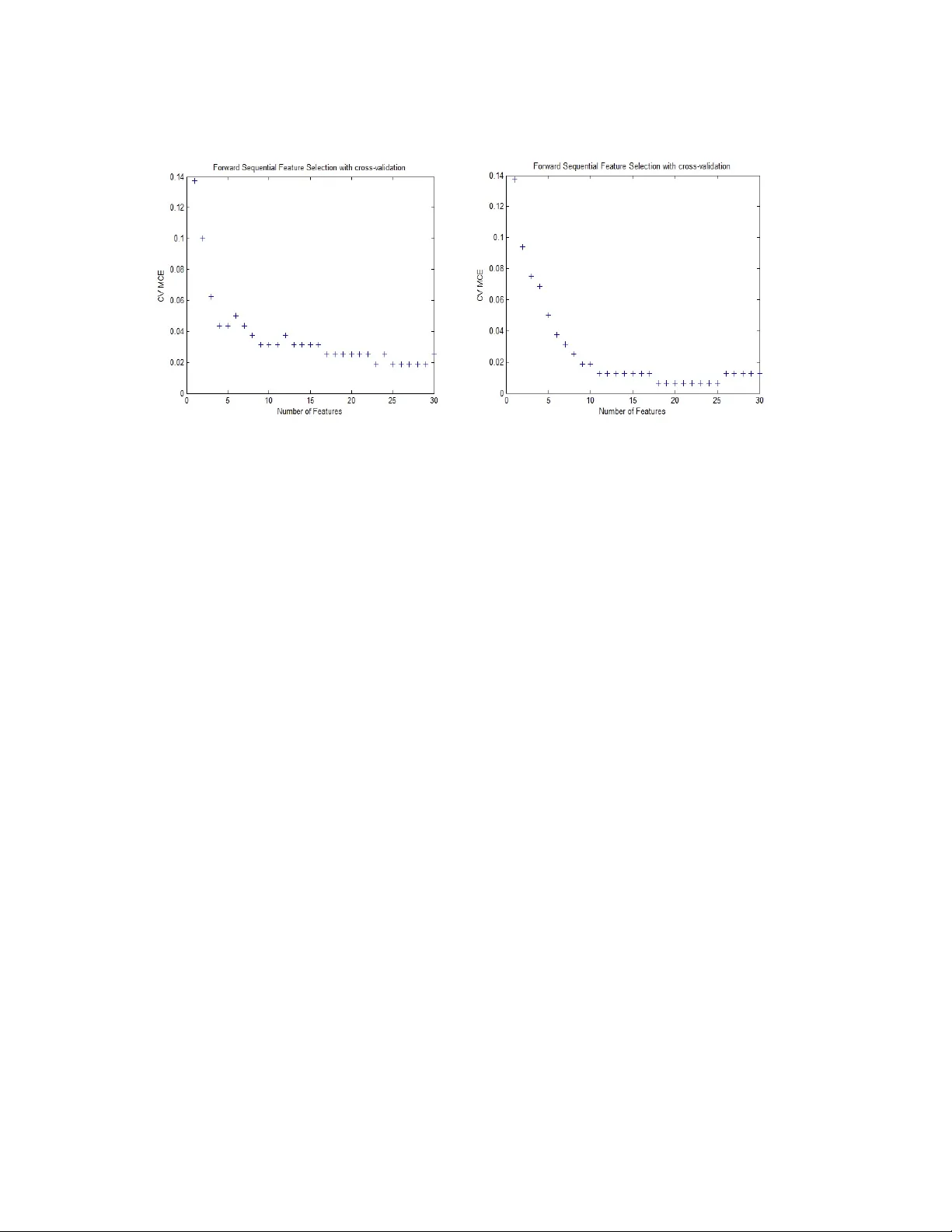
Feature Selection Using Classifier in High Dimensional Data Shivani Pathak and Vijendra Si ngh Department of Computer Science , Faculty of Engineering and Technology , Mody Institute of Technology and Science, Lakshmangarh, Rajasthan, India-332311 Abstract Feature selection is frequently used as a pre-processing step to m achine learning. It is a process of choosing a subset of original feat ures so that the feat ure space is optimally reduced according to a certain evaluation crite rion. The central objective of this paper is to reduce the dimension of the data by findi ng a small set of im portant features which can give good classification performance. We have applied filter and wrapper approach with different classifiers QDA and LDA re spectively. A widely-used filter method is used for bioinformatics data i.e. a univariat e criterion separately on each feature, assuming that there is no interaction betw een features and then applied Sequential Feature Selection method. Experimental result s show that filter approach gives better performance in respect o f Misclassification E rror Rate. Keywords: Feature Selection; QDA; L DA; Missclassification Error Rate 1. INTRODUCTION 1.1 Feature Selection In modeling problems, the analy st is often f aced with more predicto r variables than can be usefully employed. Consider that the size of the input space (the space defined by the 2 input variables in a modeling problem ) grows exponentially. Cutting up each input variable's scale into, say , 10 segments im plies that a single-input model will requ ire 10 examples for model construction, w hile a mode l with two input variables will require 100 (= 10 x 10), and so forth (assuming only one training example per cell). Assuming that the inputs are completely uncorrelated, si x input variables, by th is criterion, would require 1 million examples. In real problem s, input variables are usually som ewhat correlated, reducing the number of needed ex amples, but this prob lem still explodes rapidly, and these estimates can be considered somewhat conservative in that perh aps more than one example should be available from each cell. Given this issue, data miners are often faced with the task of selecting w hich predictor variables to keep in the model. This pr ocess goes by several names, the most common of which are subset selecti on, attribute selection and f eature selection. Many solutions have been proposed for this task, though none of them are perfect, except on very small problems. Most such solutions attack th is problem directly, by experim enting with predictors to be kept. When applied in bi ology domain, the tech nique is also called discriminative gene selecti on, which detects influential genes based on DNA microarray experiments. By removing m ost irrelevant a nd redundant features fr om the data, feature selection helps improve the perf orm ance of learning models by: • Alleviating the effect of the curse of dim ensionality. • Enhancing generalizatio n capability. • Speeding up learning process. • Improving model interpretability. 1.2. Methods used for feature selection • Filter Method • Wrapper Method • Hybrid Method Filter Method: The filter approach requires the statistical analys is of the feature set only for solving the FS task without utilizing any learning model [6]. The filters work fast using a simple measurem ent, but its result is not al ways satisfactory. Wrapper Method: The wrapper approach invo lves with the predetermined learning model, selects features on m easuring the lear ning perform ance of th e particular learning model. Hybrid Method: The hybrid approach attemp ts to take ad vantage of the filter and wrapper approaches [6, 12]. It is often f ound that, hybrid technique is capable of locating a good solution, while a single techni que often traps into an immature solution. In the Hybrid approach filter models can be c hosen as the preliminar y screening to remove the most redundant or i rrelevant features for ex. F -score and information gain. These two resulted feature sets are com bined together as the pre-processed featu re set for fine tuning. This step is called the co mbination model [7]. Finally, the wrapper model is applied to improve the class ificati on accuracy, and this is the fine-tuning step. 2. RELATED WORK Stream wise feature selection [1] consider s new features sequentially an d adds them to a Predictive model. Here a ll features are known in advan ce. Thus, the flexibility that stream wise regression provi des to dynamically decide whic h features to generate and add to the feature stream provides potentially large savings in computation. Empirical tests show that for the smaller UCI data sets where stepwise regression can be done, 4 stream wise regression gives com parable resu lts to stepwise regression or techniques such as decision trees, neural networks, or SVMs. A new hybrid genetic algorithm for feature selection is introduced called as HGAFS [2]. This algorithm selects sa lient feat ure su bset within a reduced size. HGAFS incorporates a new local sear ch operation that is devised and embedded in HGA to fine- tune the search in feature selection process. The aim is to guide the search process so that the newly generated offspring can be adjusted by the less correlated (distinct) features consisting of general and special char acteristics of a given dataset. Thus, this algorithm reduces redundancy of inform ation among the selected features. A stochastic algorithm based on the GRASP [3] meta-heurist ic is been proposed, with the main goal of speeding up the feature subset selection process, ba sically by reducing the number of wrapper evaluations to car ry out. GRASP is a multi-start cons tructive method which constructs a solution in its firs t stage, and then runs an improving stage over that solution. Several instances of th e proposed GRASP method are experim entally tested and compared with state-of-the-art algorithm s over 12 high-dimensional datasets. The complexity, in terms of wrapper eval uations carried out, of the proposed GRASP algorithm comes from the following parameters: n, the number of predictive variables; m the cardinality of the subset selected fo r the constructive step; k the number of iterations carried out by the grasp algorithm; and, the wrapper FSS method selected for the improving step. A hybrid algorithm, SAGA [4], is proposed fo r this task. SAGA combines the ability to avoid being trapped in a local minimum of simulated annealing with the very hig h rate of convergence of the crossover opera tor of genetic algorithms, the strong local search ability of greedy algorithms and the hi gh com putational effici ency of generalized regression neural networks. The performa nce of SAGA and well-known algorithms on synthetic and real datase ts are compared. 3. FEATURE SELECTION ALGORI THM WITH CL ASSIFIER Reducing the number of features (dimensionalit y) is important in statistical lea rning. For many data sets with a large num ber of features and a limited number of observations, such as bioinformatics data, usually many features are not useful for producing a desired learning resu lt and the limited observati ons may lead the learning algorithm to overfit to the noise. This pape r shows how to perfor m sequential feature selection, which is one of the most popular f eature selection algorit hms. It also shows how to use holdout and cross-validation to ev aluate the performan ce of the selected features. 3.1 Discriminant Analysis Method (Classifier) • QDA(Quadratic Discriminant Analysis) • LDA(Linear Discriminant Analysis) Quadratic discriminant analysis (QDA) is closely related to linear discriminant analysis (LDA), where it is assumed that there are only two classes of points and that the measurements are normally distributed. Unlike LDA however, in QDA there is no assumption that the covariance of each of th e classes is identical. When the assum ption is true, the best possible test for the hypothe sis that a given measurement is from a given class is the likelihood ratio test. 6 Linear discriminant analysis (LDA) is used in statistics, patter n recognition and machine learning to find a linear combination of features which characterizes or separates two or more cl asses of objects or events. The resulting combination may be used as a linear clas sifier or, m ore comm only, for dimensionality reduction before later classif ication. LDA explicitly attemp ts to model the difference between the classes of data. 3.2 Validations Used 3.2.1 Hold-out Validation The holdout m ethod is the simplest kind of cr oss validation. The da ta set is separated into two sets, called the training set a nd the te sting set. The function approximator fits a function using the training set only. Then the function approximator is asked to predict the output values for th e data in the testing set (it has never se en these output values before). The errors it makes are accumulated as before to give the m ean absolute test set error, which is used to evaluate the model. 3.2.2 Cross Validation Cross-validation [1], sometimes called rotation estimation, is a technique for assessing how the results of a statistical anal ysis will genera lize to an independent data set. In k -fold cross-validation, th e original sample is random ly partitioned into k subsamples. Of the k subsamples, a single subsample is retained as the validation data for testing the model, and the remaining k − 1 subsamples are used as training data. The cross-validation pro cess is then repeated k times (the folds ), with eac h of the k subsamples used exactly onc e as the validation data. The k results from the fo lds then can be averaged (or o therwise combined) to produce a s ingle estim ation. In stratified k -fold cross-validation, the folds are se lected so that the mean response value is approximately equal in all the f olds. In the case of a dichotomous class ification, this means that each fold contains roughly the same proportions of the two types of class labels. 3.4 Algorithm (Sequential Feature Selection) Sequential forward selection (SFS) and se quential backward selection (SBS) are commonly used algorithms, us ually in com bination with a wrapper evaluator. Both algorithms have O (n 2 ) worst-case complexity, but especially in high-dimensional datasets only SFS is used because the evalua tions are simpler (few er variables in the selected subset). SFS is a bottom up search procedure that adds new features to a feature set one at a time until the final feature set is reac hed. Suppose we have a set of d 1 features X d1. For each of the feature yet not selected ξ j (i.e. in X- X d1 ) the criterion function J j = J (X d1 + ξ j ) is evaluated. The feature that yields the maximum value of J j is chosen as the one that is added to the set X d1. thus at each stage the variable is chosen that, when added to the current set, maximises the selection criterion. The feature set is in itialised to the null set. When the best improvement m akes th e feature set worst, or when the m aximum allowable number of feature is reached, the algorithm terminates. Here J can be given by J= X k T .S k -1 .X k where X k is a k dimensional vector and S k is a k*k positive definite matrix when k features are used. Following algorithm explains the whole procedure, at each stage of the search, sets of subsets are generated for evaluation using the cross validation procedure. Variable ξ j is chosen for which J(X- ξ j ) is the largest. The new set is (X- ξ j ). This process is repeated until the set of required cardinality rem ains. 8 Cross Validation algorithm for selection of the be st set of f eatures in a sequential sear ch procedure is explained as follows: ALGORITHM 1. Divide the data into training and test set. 2. Specify the search strategy (here SFS). At each stage of the algorithm: (a) Generate subsets of f eature for evaluation. (b) Cross-validation procedure: i. Split the training data into e.g. 10 equal parts, ensuring that all classes are represented in each par t; use nine parts for training and remaining one part for testing. ii. Train the classifier model for each nested subset of variable, S h, on each subset, k, of the training data in turn, testing on the remaining part. Obtain the performance for e.g. error rate, CV(h, k), h=1, …,p; k=1, … , 10 iii. Average the result ; ) , ( 10 1 ) ( ∑ = k k h CV h CV CV: Cross Validation 3. Select the smallest feature subset, S h* , such that CV (h) is optimal or near optimal. 4. Evaluate on test dataset us ing the feature subset S h*, training on the entire training set and evaluating pe rformance on the test set. 4. EXPERIMENTAL RESULTS We used a clinical high dimensional da ta here which have 216 rows and 4000 features. The data variable consists of 216 observations with 4000 features. Here, we divide data into a training set of size 160 and a test set of size of size 56. We use Quadratic Discriminant Analysis (QDA) a nd Linear Discriminant Analysis (LDA) separately on the sam e dataset as the classi fication algor ithm. In th is paper we explained one example of a filter method and one exam ple of a wrapper method. A widely-used filter method for bioinformatics data is to ap ply a univariate criterion separately on each feature, assuming that there is no interacti on between features. For example, we might apply the t-test on each feature and compar e p-value (or the absolute values of t- statistics) for each feature as a measure of how effective it is at separating groups. In order to get a general idea of how well-separ ated the two groups are by each feature, we plot the empirical cumulative distribution f unction (CDF) of the p-values. In the graph obtained after classification(Fi g 1 (a);(b) ) there are about 35% of features having p- values close to zero and 50% of features having p-values smaller than 0.05, meaning there about 2000 features among the orig inal 4000 features that have strong discrimination power. Fig. 1. (a) QDA (b) LDA 10 We can sort these features according to their p-values (or the absolu te values of the t- statistic) and select some features from the sorted list. However, it is usually diff icult to decide how many features are needed unl ess one has some domain knowledge or the maximum number of features that can be cons idered has been dictated in advance based on outside constraints. One quick way to decide the number of needed features is to plot the MCE (misclassification error, i.e., the num ber of misclassified observations divided by the number of observations) on the test se t as a function of the number of features. Since there are only 160 observation s in the training set, th e larges t number of features for applying QDA and LDA is limited, otherwis e, there may not be enough sam ples in each group to estimate a covariance m atrix. Actu ally, for the data used in this p aper, the holdout partition and the sizes of two groups dictate that th e largest allowable number of features for applying QDA is about 70. Now we compute MCE for various numbers of features between 5 and 70 and show the plot of MCE as a function of the number of features. In order to reasonably estimate th e performance of the se lected model, it is important to use the 160 training samples to fit the QDA and LDA model and compute the MCE on the 56 test observa tions. This simple filter feature selection method gets the smallest MCE on the test set when 20 f eatures and 60 features are used in QDA and LDA respectively. The plot (Fig. 2 (a), (b)) shows overf itting occurs when more than these features are used. The training set is used to se lect the features and to fit the QDA model, and the test set is used to evaluate the performance of the finally selected feature. During the featu re selection procedure, to eval uate and to compare the perf ormance of the each candidate feature subset, we apply stratified 10-fold cro ss-validation to the trai ning set. Then we use the filter results as a pre- processing step to select feat u res. For example, we select 150 features here. We apply forward sequent ial feature selection on these 150 features. It stops when the first local minimum of the cross-valida tion MCE is found. The algorithm may have stopped prematurely. So m etimes a smalle r MCE is achievable by looking for the minimum of the cross-valid ation MCE over a reasonable range of number of features. The cross-validation MCE (QDA),as shown in fig.3(a) reaches the minimum value when 9 features are used and this curve stays f lat over the range from 9 features to 27 features (excep t for a slight increase when 22 features are u sed). Also the curve goes up when more than 28 features are used, which means overfitting occurs there. It is usually pref erable to have fewe r features, so h ere we pick 9 features, and calculated Fig. 2. (a) QDA (b) LDA the final Misclassification Error that comes out to be 0.0714. Same procedure when applied using LDA Misclassif ication Error comes out to be 0.0893 when 9 features are picked as shown in fig.3 (b). Table 1. Misclassification Error Approach QDA LDA Simple Feature Selection 0 .0536 0.0200 Sequential Feature Selection 0.0714 0.0893 12 Fig. 3. (a) QDA (b) LDA 5. CONCLUSION Misclassification error rate (the number of m isclassified ob serv ations divided by the number of observations) is ca lculated in this paper to decide the number of needed features using holdout validatio n and cross-validation. In or der to reasonably estimate the performance of the selected model, we used 160 training samples to fit the model and compute the MCE on the 56 test observations. Simple Filter Feature Selection m ethod gets the sm allest MCE on the test set when 20 features are used in QDA and 15 features are used in LDA. The plot shows overfitting occurs when more than these features are used. REFERENCES [1 ] Jing Zhou, Dean P. Foster Robert A. Stine, Lyle H. Ungar, Streamwise Feature Selection, Journal of Mach ine Learning Research , 2006, pp 1861-1885 [2] Md. Monirul Kabir, Md. Shahjahan, Kazuyuki Murase , A New Local Search based Hybrid Genetic Algorithm for Feature Selection, Neurocomputing, Vol.74, Issue 17 ,2011, pp.2914-2928 [3] Pablo Bermejo, Jose A. Gámez, Jose M. Puerta, A GRASP algorithm for fast hybrid (filter-wrapper) feature subset selection in high-dimensional datasets, Pattern Recognition Letters ,2011, pp 701–711 [4] Iffat A.Gheyas, Leslies. S mith, Feature subset sele ction in large dimensionality domains, Pattern Recognition, 20 10, pp 5 – 13 [6] M. Dash, H. Liu, Feature selecti on for classification, Intellige nt Data Analysis 1 (1997), pp 131–156. [7] Hui-Huang Hsu, Cheng-Wei Hsieh, Ming-Da Lu, Expert Systems with Applications, 38 (2011), pp 8144–8150. [8] I. Guyon, A. Elisseeff, An introduc tion to variable an d feature selection, Journal of Machine Learni ng Research 3 (2003), pp 1157–1182. [9] J. Huang, Y. Cai, X. Xu, A hybrid genetic algorithm for feature selection wrapper based on mutual information, Pa ttern Recognition Letters 28 (2007), pp 1825–1844. [10] J. Kittler, “Feature Set Search Algorithms,” Pattern Recognition an d Signal Processing, C.H. Chen, ed., 1978, pp. 41-60. 14 [11] R.K. Sivagaminathan, S. Ramakr ishnan, A hybrid approach for feature subset selection using neural networks and ant colony optimization, Expert Systems with Applications 33 (2007), pp 49–60.