Unsupervised learning of depth and motion

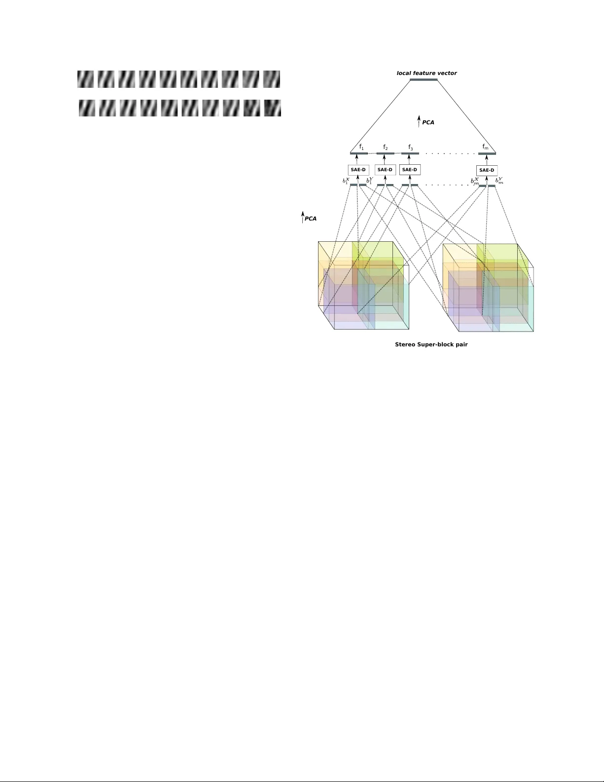
Unsupervised learning of depth and motion Kishore K onda Goethe Uni versity Frankfurt Germany konda@informatik.uni-frankfurt.de Roland Memise vic Uni versity of Montreal Canada roland.memisevic@umontreal.ca Abstract W e pr esent a model for the joint estimation of dispar- ity and motion. The model is based on learning about the interr elations between images fr om multiple cameras, mul- tiple frames in a video, or the combination of both. W e show that learning depth and motion cues, as well as their combi- nations, fr om data is possible within a single type of arc hi- tectur e and a single type of learning algorithm, by using bi- ologically inspir ed “complex cell” like units, which encode corr elations between the pixels acr oss image pairs. Our experimental r esults show that the learning of depth and motion makes it possible to achieve state-of-the-art perfor- mance in 3-D activity analysis, and to outperform existing hand-engineer ed 3-D motion featur es by a very lar ge mar- gin. 1. Introduction A common property of 3-D inference and motion esti- mation is that both rely on establishing correspondences between pixels in two (or more) images. For depth esti- mation, these are correspondences between multiple vie ws of a scene, for motion estimation between multiple frames in a video. Despite superficial differences between these tasks, such as the typical size of the average displacement across images, or whether the geometry is constant or vari- able across pairs, there are much stronger commonalities between the tasks, such as the fact that both rely on finding positions in one image which match those in another im- age. This suggests that both tasks may be learnable using essentially the same type of architecture and the same type of learning algorithm, but there has been hardly any work on trying to exploit this in practice. Besides the obvious advantage of allowing us to dev elop and maintain a single piece of code to achie ve both tasks, it makes it trivial to fuse the information from both sources and thereby to design ar- chitectures that learn representations of multi-camera video streams with application, for example, in acti vity analysis. In the neuroscience literature, the so-called comple x cell “energy model”, is assumed to be the main underlying mechanism behind both depth and motion estimation (e.g. [1, 3]), and it provides an elegant explanation for ho w the brain can learn both using the same type of neural hardw are. There has been some progress recently in learning mo- tion energy models from data [10, 17], and learning based methods are among the state-of-the-art in acti vity analysis from videos. Ho wev er , there has been hardly any work on learning energy models for depth inference, nor for learn- ing depth and motion information at the same time. In this work we sho w that it is, in fact, possible to learn about 3-D depth entirely unsupervised from data, similar to learning motion as done using complex cell type models. Our ex- periments sho w how this makes it possible to achie ve state- of-the-art performance in 3-D activity analysis from multi- camera video without making use of any hand-crafted fea- tures. 1.1. Biologically inspired models of correspondence The first step to infer depth from tw o views is to find cor - respondences between points which represent the same 3-D location [7]. The two standard ways to approach this task are: 1.) For each position in one image find a nearby match- ing point in the other image using some measure of similar - ity between local image patches (e.g. [16]). 2.) For each position in both images, e xtract features that describe phase and frequency content of the re gion around that point, and read off the phase dif ference across the two images from the set of filter responses [14]. The first approach has been more common in practice, although the second is more biologically plausible, as it does not require loops ov er local patches. More importantly , the second approach is amenable to data-driven learning as we shall show . The most well-known account of phase- based disparity estimation is the binocular energy or cross- correlation model (e.g. [14, 4, 13]). In its most basic form, this model states that local disparities are encoded in the sum of the squared responses of two neurons, each of which has a binocular receptiv e field. Each binocular receptiv e field, in turn, sho ws a position-shift across the two views. 1 Between them the two receptive fields show a quadrature relationship (within each view). It can be shown that the position-shift across the views allo ws the energy model to encode local disparity , while the quadrature relationship within each view allo ws it to be independent of the Fourier phase of the local stimulus [14, 3]. Analogous models, also based on energy or cross- correlation, have been proposed independently for motion encoding [3, 2, 12]. This is not surprising if one considers that motion can be defined as the transformation of a giv en input ov er time and disparity as the transformation of the in- put across multiple vie ws or a stereo pair . If the gi ven input is a set of frames from a time sequence the model encodes motion and when the input is a stereo pair it encodes dispar - ity . It has been proposed that, due to similarity of models for motion and disparity encoding, it should be possible to integrate them [14]. But to date, there has been no practical exploration of this idea, nor of the learning of depth from data. In this paper we present an approach to learning depth, motion and their combination from data, by using a fea- ture learning architecture based on the energy model. Our approach is based on the view of energy model proposed by [9], which shows that the (motion) energy model can be viewed as two independent contributions to motion encod- ing: 1) the detection of spatio-temporal “synchrony”, and 2) the encoding of inv ariance. [9] present an autoencoder model using multiplicativ e interactions for detection of syn- chrony , and they show that a pooling layer independently trained on the hidden responses can be used to achiev e con- tent in v ariance. W e adopt that approach for the estimation of depth and motion cues, as it gives rise to an ef ficient single-layer learning algorithm. But there a variety of learn- ing based energy models that one could use instead (e.g., [10, 17]). A description of the synchrony condition and how it can be used for implicit encoding of depth is presented in the next section. Since depth is encoded implicitly in the fea- ture responses of the model, we then show how it is possible to “calibrate” an energy model learned on stereo data us- ing a vailable ground truth data to compute an explicit depth map from this encoding. Since in most applications, the representation of depth is a means to an end not a goal on its o wn, we then explore a v ariety of ways to utilize the im- plicit encoding of depth, as well as motion, using the same approach to learning features. W e ev aluate and compare sev eral v ariations of this approach on the Hollyw ood3D ac- tivity recognition dataset [6], and we demonstrate that it im- prov es significantly upon the state-of-the-art, using a mini- mum of hand engineering. 2. Depth as a latent variable The classic energy model (e.g. [1, 3]) states that we can obtain an estimate of the transformation, P , between two images ~ x 1 and ~ x 2 by computing a weighted sum over prod- ucts of filter responses on the images. In particular , if the filters themselves dif fer by the transformation P , so that, ~ w 2 = P ~ w 1 (1) then the product filter responses will be large for input im- ages for which ~ x 2 = P ~ x 1 holds, too. This makes it possible to extract motion, if ~ x 1 and P ~ x 2 denote adjacent frames in a video, and disparity if they denote tw o patches cropped from the same position of a stereo pair . In most practical sit- uations (for both motion and disparity estimation), the dom- inant transformation between the images is a local transla- tion , in which case the optimal filters are Gabor features and P is a small phase shift. In early , biologically moti- vated approaches to estimating displacements, filters hav e been hand-coded [1, 3]. In the context of motion estima- tion, v arious approaches were proposed recently to learning the filters from data (e.g. [17, 10, 11]). While learning has been inefficient due to the vast amounts of image patch pairs required for learning good filters, [9] recently presented the “synchrony autoencoder”, which learns motion representa- tions more efficiently , using a single-layer autoencoder with multiplicativ e interactions. W e use a similar approach for defining models that learn to encode depth. W e shall revie w that model, as well as sho w ho w we can use it for depth and motion estimation in the following section. 2.1. Depth across stereo image pairs Based on the abov e description, we can define a model based on the synchrony autoencoder (SAE) [9] for learning depth representation from stereo pair of images as follows. Assume we are giv en a set of stereo image pairs, ~ x, ~ y ∈ R N . Let W x , W y ∈ R Q × N denote the matrices containing Q feature vectors ~ W x q , ~ W y q ∈ R N , stacked ro w-wise. W e define the latent representations ~ f x = W x ~ x and ~ f y = W y ~ y , which are typically called factors in the con- text of energy models [17, 11, 9]. The hidden representation of disparity is then defined as ~ h = σ ( ~ f x  ~ f y ) (2) where σ = (1 + exp( − x )) − 1 is a saturating non-linearity . (W e use the logistic sigmoid in this work, but other non- linearities could be used as well.) A standard way to train an autoencoder is by minimiz- ing reconstruction error . Since the vector of multiplicativ e interactions between factors represents the transformation between x and y , here we may define the reconstruction of Figure 1: A model encoding the transformation inherent in the image pair ( ~ x, ~ y ). one input giv en the other input and the transformation as ˆ x = ( W x ) T ( ~ h  ~ f y ) (3) ˆ y = ( W y ) T ( ~ h  ~ f x ) (4) Here, we assume an autoencoder with tied weights similar to [17, 11, 9]. This allows us to define the reconstruction error the as symmetric squared difference between inputs and their corresponding reconstructions: L (( ~ x, ~ y ) , ( ˆ ~ x, ˆ ~ y )) = k ( ~ x − ˆ ~ x ) k 2 + k ( ~ y − ˆ ~ y ) k 2 (5) 2.1.1 Regularization For extraction of sparse and robust representation we use contraction as regularization [15] which amounts to adding the Frobenius norm of the Jacobian of the hiddens with re- spect to the inputs x, y . k J e ( ~ x, ~ y ) k 2 E = X ij  ∂ h j ( ~ x, ~ y ) ∂ x i  2 + X ij  ∂ h j ( ~ x, ~ y ) ∂ y i  2 (6) Using sigmoid non-linearity the contraction term becomes k J e ( ~ x, ~ y ) k 2 E = X j ( h j (1 − h j )) 2 ( f x j ) 2 X i ( W x ij ) 2 + X j ( h j (1 − h j )) 2 ( f y j ) 2 X i ( W y ij ) 2 (7) Thus the complete objecti ve function employing con- tractiv e regularization, using λ as the regularization strength, is J C = L (( x, y ) , ( ˆ x, ˆ y )) + λ k J e ( x, y ) k 2 E (8) T o obtain filters that represent depth we minimize Eq. 8 for a set of image pairs cropped from identical positions of multiple views of the same scene. It is important to use a patchsize that is large enough to cov er the maximal dis- parity in the data, otherwise the model will not be able to encode the corresponding depth. In contrast to traditional approaches to estimating depth, howe ver , there is no need for rectification, since the model can learn any transforma- tion between the frames not just horizontal shift. 2.2. Depth across stereo sequences In the previous section we described a model for en- coding depth across stereo image pairs. W e no w propose sev eral extensions of this approach to learn representations from stereo sequences not still images. This makes it possi- ble to e xtract a representation informed by both motion and depth from the sequence. W e defer the detailed quantitativ e ev aluation of the approaches to Section 3. 2.2.1 Encoding depth Let ~ X , ~ Y ∈ R N be the concatenation of T v ectorized frames ~ x t , ~ y t ∈ R M , t = 1 , . . . , T , and be defined such that ( ~ x t , ~ y t ) are stereo image pairs. Let W x , W y ∈ R Q × N de- note matrices containing Q feature vector pairs ~ W x q , ~ W y q ∈ R N stacked ro w-wise. Each feature is composed of indi- vidual frame features ~ w x q t ∈ R M each of which spans one frame ~ x t from the input sequence. Accordingly for the fea- tures in W y . In analogy to the pre vious section, we can define the fac- tors ~ F X = W x ~ X and ~ F Y = W y ~ Y corresponding to the sequences ~ X , ~ Y . A simple representation of depth may then be defined as H D q = σ ( F x q · F y q ) (9) The representation H D q will contain products of frame responses  ( ~ w x q t ) T ~ x t  ·  ( ~ w y q t ) T ~ y t  which detect syn- chrony over stereo pairs encoding depth. It will also contain products across time and position,  ( ~ w x q t ) T ~ x t  ·  ( ~ w y q ( t + i ) ) T ~ y t + i  , which will weakly encode motion as well. In other words, motion is encoded indirectly by this model, by computing products of responses at different times across cameras. W e shall refer to this model as SAE- D for “depth encoding synchrony autoencoder” in the fol- lowing. 2.2.2 Encoding motion For analyzing the effect of encoding motion vs. depth on the classification of sequences, we can define a hidden rep- resentation which employs only a single stereo sequence as follows. Let ~ X = ~ Y represent a single camera channel from the stereo sequence. If we tie the weight matrices W x , W y to be identical as well, Eq. 9 may be rewritten H M q = σ (( F x q ) 2 ) (10) Since F x q is the sum over individual frame filter responses, its square, by the binomial identity , will contain products of individual frame responses across time  ( ~ w x q t ) T ~ x t  ·  ( ~ w x q ( t + i ) ) T ~ x t + i  as well as the squares of filter responses on indi vidual frames. H M q will therefore take on a large value only for those filters which match all indvidual frames, which implies that they will jointly satisfy Eq. 1. This observation is the basis for the well-known equi valence between the energy model and the cross-correlation model (see, for example, [3, 12, 9]). Thus, in this case synchrony is detected over time, en- coding the motion present in the input sequence. In anal- ogy to the previous section, the encoding of motion will be weakly related to depth in the scene, as well, because depth and motion tend to be correlated. Any camera mo- tion, for example, may be viewed as providing multiple views of a single scene, thereby implicitly containing in- formation about depth (a fact that is exploited in structure- from-motion approaches). Howe ver , due to the absence of camera motion which is consistent across the dataset, as well as the presence of a multitude of object motions, the depth information will only be weakly present in any en- coding of motion. W e shall call this model for representing motion SAE-M in the follo wing. The model is equiv alent to the SAE defined in [9] for encoding motion from a single- channel video. 2.2.3 Multiview disparity T o obtain an explicit encoding of both depth and motion, we require the detection of synchrony both across time and across stereo-pairs. One w ay to obtain such a representation in practice is to combine the representations defined in the previous two sections, for example, by using their av erage or concatenation. As a third alternativ e, we propose defining a joint rep- resentation by including products of frame responses across both time and stereo-pairs. Recall that the square of the sum ov er frame-wise filter responses contains within-channel motion information. W e suggest obtaining an estimate of the across-channel disparity information by defining the hidden unit response as the product ov er theses squares. This allows us to extract information about disparity from the relation between the temporal e volutions of the com- plete video sequence, rather than between feature positions across single frames. T o this end, we define the hidden rep- resentation H M D q = σ (( F x q ) 2 · ( F y q ) 2 ) (11) The representation H M D q may be written as  P ( ~ w x q t ) T ~ x t  2 ·  P ( ~ w y q t ) T ~ y t  2 , and it may be thought of Figure 2: Filters learned on stereo patch pairs from the KITTI dataset. as a “multi-vie w” or “motion-based” estimate of disparity . W e call a model based on this representation of disparity SAE-MD in the following. 2.3. Learning For the models described abo ve the decoder and recon- struction cost can be deriv ed to be similar to that of stereo- pair model in Section 2.1. In particular , the reconstruc- tion error and contraction cost for the models SAE-D and SAE-M can be derived by replacing the corresponding pa- rameters of Equations 5 and 7. For the SAE-D model this amounts to replacing frames ~ x, ~ y with sequences ~ X , ~ Y , and for the SAE-M model to further substituting ~ X for ~ Y . For the SAE-MD model, we found the contraction cost to be unstable due to presence of higher exponents in the hidden representation. Because of this, we use the trained weights from the SAE-D model and during inference use the representation from Equation 11. Alternatively it may be possible to train the model using a denoising criterion instead of contraction for regularization. 2.4. Interest point detector Hand-crafted image, motion or 4-D descriptors are typ- ically accompanied by corresponding interest point detec- tors. Since they reduce the number of positions to extract representations from, they hav e been shown to improve ef- ficiency and performance, for example, in bag-of-features based recognition pipelines. For a learned representation that is based on the linear projection of image patches, it is possible to define a default interest point operator, by using norm-thresholding of fea- ture activ ations (see, for example, [10]). It can be moti vated by the observation that norms of relev ant features will be higher at edge and motion locations than at homogeneous or static locations [8]. Norm thresholding interest point de- tection amounts to simply discarding features H with norm | H | 1 < δ . The v alue of δ may be chosen based on the mean norm of the features in the training set. 3. Experiments 3.1. Learning depth from image pairs It has been well-known that energy and cross-correlation models with hand-crafted Gabor features are able to ex- tract depth information from random-dot stereograms (e.g., [14]). In order to test whether depth information can be extracted in more realistic settings and using features that are learned from data, as proposed in Section 2, we first conducted an experiment where a depth map is estimated giv en a stereo image pair . For this experiment we use stereo images from the KITTI stereo/flow benchmark [5]. The dataset consists of 194 training image pairs and 195 test image pairs. For the training image pairs corresponding ground truth depth is provided. Since the ground truth is captured by means of a V elodyne sensor which is calibrated with the stereo pair it is only provided for approximately 30% of their image pixels. W e down-sampled the images from a resolution of 1226 × 370 pixels to 300 × 100 pix- els, so that the local shift between image pairs falls within the local patch size, which is a crucial requirement for mod- els using local phase matching for disparity computation as discussed in Section 2. W e trained the stereo-pair model described in Section 2.1 (Eq. 2) on patch pairs cropped from the training set. Each patch is of size 16 × 16 pixels and the total number of train- ing samples is 100 , 000 . The patches used for learning the filters are cropped only from regions of images where cor- responding depth information is av ailable. Some learned filters are shown in Figure 2. The figure shows that filters are localized, Gabor-like and span a wide range of frequencies and positions. Since cameras are par- allel the filters learned predominantly horizontal shifts. T o test if we can extract depth information from the learned hidden representation, we trained a logistic regres- sion classifier using the a vailable ground truth as the output data. T o this end, we generate labels by taking the mean ov er non-zero pixel intensities of corresponding patches from the ground truth, which we then quantize into 25 bins. After training the classifier, estimation of depth for a giv en stereo pair in volves dense sampling of patch pairs followed by feature computation and prediction by the classifier . A sample stereo image pair and the learned depth map is shown in Figure 3. In the figure, each predicted depth label is one pixel of the estimated depth map. An artif act of this depth estimation procedure is that object boundaries are expanded over their actual size due to the patch size used in the model. It can be also observed that the depth for feature- less re gions like sky and plane surf aces is less accurate than in feature rich re gions, because the model cannot detect any shift in those cases. This is true, of course, for any disparity estimation scheme based on local region information, and when the (a) Left image (b) Right image (c) Depth Map (d) Depth map masked using interest points Figure 3: Stereo image pair and estimated depth maps. Depth map scale ranges from 1 (Far , shown as black) to 25 (Near , shown as white). goal is an explicit depth map, one should use a Markov Random Field or similar approach to cleaning up the ob- tained depth map. In the e vent where one is not interested in an e xact depth map, b ut rather in depth cues to help make predictions that merely depend on depth (similar to the bag- of-features approach taken typically in motion estimation), a possible alternative is the use of an interest point detector as explained in Section 2.4. Figure 3c shows an e xample of an estimated depth map with interest points, and it shows that norm thresholding masks out most of the re gions pre- dominantly homogeneous regions in the image. In general, we thus observe that it is possible to infer depth information from the filter responses defined in Sec- tion 2, even if the information comes in the form of noisy cues, similar to most common estimates of motion, rather than in the form of a clean depth map. W e shall discuss an approach to exploiting this information in a bag-of-features W X q W Y q Figure 4: Example of a filter pair learned on sequences by the SAE-D model from the Hollywood3D dataset. pipeline for activity recognition in the ne xt section. 3.2. Activity Recognition W e ev aluate the effect of implicit depth encoding on the task of activity recognition, using the Hollywood3D dataset introduced by [6]. The dataset consists of stereo video sequences along with computed depth videos. The videos are of 14 different categories with 643 videos for training and 302 for testing. The different categories are ’Run’, ’Punch’, ’Kick’, ’Shoot’, ’Eat’, ’Driv e’, ’UsePhone’, ’Kiss’, ’Hug’, ’StandUp’, ’SitDown’, ’Swim’, ’Dance’ and ’NoAction’. The videos are do wnsampled spatially from size of 1920 × 1080 to 320 × 240 . Models are trained on PCA whitened spatio-temporal block pairs with each block of size 10 × 16 × 16 . 300 , 000 samples are used for train- ing and the number of hidden units is fixed for all mod- els to 300 . A sample feature pair learned by the SAE-D model is sho wn in Figure 4. Each filter in the pair spans ten frames. The filters are again Gabor-like and show a continu- ous phase shift through time, and another phase shift across camera views. For the quantitativ e e valuation, we use the frame work presented by [6]. After performing feature extraction, we perform K-means v ector quantization followed by a multi- class SVM with RBF kernel for classification. A flow dia- gram of the pipeline is visualized in Figure 6. Feature are extracted using a con volutional architecture similar to that presented in [9, 10]. Super block pairs of size 14 × 20 × 20 pixels each are cropped densely with stride (7 , 10) in time and space, respecti vely , from the stereo video pairs. From the super blocks, sub-blocks of the same size as the training block size ( 10 × 16 × 16 pixels) are cropped with stride (4 , 4) , resulting in 8 sub-blocks per super block. W e first compute the feature vector for each stereo sub- block pair . W e then concatenate feature vectors correspond- ing to the sub-blocks of a super block and reduce their di- mensionality using PCA. This procedure, using the SAE-D model as an example, is visualized in Figure 5. The number of words for K-means vector quantization is set to 3000 . Our main goal in these experiments is to ev aluate the impact of the implicit depth encoding in the task of activity recognition. W e compare a variety of settings to this end. In experiment 1 , the SAE-D is used for feature extraction. As we discussed in Section 2 the SAE-D primarily encodes SAE-D PCA PCA loca l featu re vector f 1 f 2 f 3 f m SAE-D SAE-D SAE-D Stereo Sup er-b lock pai r Figure 5: Feature extraction framework using the SAE-D model. depth. Experiment 2 uses the SAE-M for feature extraction with only one of the stereo channels as input. Experiment 3 employs the SAE-MD for features extraction, and is thus based on a representation that integrates across-frame and across-channel correlations. In Experiment 4 we test two alternativ e ways of integrating depth and motion informa- tion, by combining the representations from two separately trained SAE-D and SAE-M models. The first, which we call SAE-MD(Ct), amounts to concatenating the represen- tations from SAE-D and SAE-M as features. The other , SAE-MD(A v), amounts to computing the a verage precision using the mean ov er confidences from experiments 1 and 2. Thus it amounts to averaging the classification decisions of two separate classification pipelines (one based primarily on depth, and the other based primarily on motion). Each configuration is ev aluated by computing the aver - age precision and the correct-classification rates. The re- sults are reported in T ables 1 and 2. W e repeated the exper - iments using the norm-thresholding interest point detector described in Section 2.4. From the results it can be observed that the combina- tion of motion and depth cues performs better than using individual cues. All results, including the motion-only , the depth-only and the combination models, outperform all ex- isting models, based on hand-crafted representations, by a Depth/ motion featur e e xtrac tion V ector qu antiza tion (k-mea ns c lusterin g) C lassification (RBF k er nel SVM) L ocal featur e vectors V ideo descriptor Class label Input video Figure 6: Flo w diagram of the classification pipeline. very large margin, and the y are to the best of our knowledge the best reported results on this task to date. It has been observed in the past that learning based features tend to outperform more traditional features, like SIFT , in object recognition tasks and, more recently and by a larger mar gin, in motion analysis tasks as compared to spatio-temporal variations of SIFT (e.g., [10, 17, 9]). This observation is confirmed in this 4-D dataset, where it seems to be ev en more pronounced. W e can also observe that models using interest points (cf., Section 2.4) provide an additional consistent (albeit smaller) improvement over those that do not. Furthermore, the use of depth information pro vides an edge o ver motion- only models. Interestingly , the overall effect of the various variations of the model differ heavily across action class, which can be seen in T able 1. For example, the AP for classes Run, Kick, Shoot and Eat are the highest when using primarily depth features for classification; NoAction and Kiss hav e best AP when using just motion features; and the AP for all the other classes is the highest when combining depth and motion features. This can be due to multiple rea- sons, and it is likely related to the av erage depth variation within the activity class. A detailed analysis of which type of information is the most useful for which type of activity class is an interesting direction for future work. A well-known and popular “recipe” to improve perfor- mance in learning tasks has been to base classification deci- sions on the combination of multiple dif ferent models, each of which utilizes a different type of feature. While this recipe often works well in practice, the main challenge to make it work is to dev elop models which are sufficiently differ ent from one another , so they yield a sufficiently lar ge reduction of v ariance. Utilizing the combination of depth and motion cues may be viewed in this context also as a way to extract cues from video data which are dif ferent, since they represent v ery different properties of the en vironment. 4. Discussion Most current practical w ork on stereopsis focuses on ex- tracting dense depth-maps using MRFs. Potential reasons Method Interest points AP CC Rate SAE-M None 24.31 29.61 SAE-MD None 24.69 29.47 SAE-D None 23.53 26.82 SAE-M N-Th 24.61 31.79 SAE-MD N-Th 25.14 30.46 SAE-D N-Th 24.05 26.49 SAE-MD(Ct) N-Th 24.45 29.47 SAE-MD(A v) N-Th 26.11 30.13 HoG/Hof/HoDG [6] 3.5D-Ha 14.1 21.8 RMD-4D[6] 3D-Ha 15.0 15.9 T able 2: Correct classification rate and av erage precision. for biology to take a different route might be that (a) depth via deep learning makes it possible to use the exact same learning algorithm for depth inference that is also used to recognize objects and motion; (b) a simple depth cue, as giv en by a feature vector , H , is often entirely suf ficient to take swift vital decisions, such as to dodge an approach- ing object; (c) learning depth inference from data allo ws for feed-forward depth perception, and thus to av oid the need for a complicated and brittle pipeline, which in volv es rec- tification, hypothesis generation, and robustification using RANSA C [7]. In this paper we sho wed how unsupervised feature learn- ing may be used to mimic this way of e xtracting depth cues from image pairs, and that learning joint representations of motion and depth within a single type of architecture and a single type of learning rule can achiev e state-of-the-art per- formance in a 3-D activity recognition task. Our work is to the best of our knowledge the first published work that shows that deep learning approaches, which hav e hitherto been shown to work well in object and motion recognition tasks, are also applicable in the domain of depth inference, or more generally to 3-D vision. Action SAE-MD SAE-MD(A v) SAE-MD(Ct) SAE-M SAE-D 3D-Ha 4D-Ha 3.5D-Ha NoAction 12.10 12.77 13.10 15.73 12.15 12.1 12.9 13.7 Run 52.56 50.44 51.45 45.38 56.07 19.0 22.4 27.0 Punch 41.09 38.01 32.68 33.86 36.17 10.4 4.8 5.7 Kick 9.41 7.94 6.86 6.63 11.84 9.3 4.3 4.8 Shoot 30.26 35.51 30.49 30.52 40.72 27.9 17.2 16.6 Eat 5.85 7.03 6.78 7.29 9.03 5.0 5.3 5.6 Drive 52.65 59.62 51.35 61.61 45.19 24.8 69.3 69.6 UsePhone 22.79 23.92 19.01 23.60 23.36 6.8 8.0 7.6 Kiss 15.03 16.40 16.12 17.86 17.06 8.4 10.0 10.2 Hug 6.64 7.02 7.61 7.38 9.27 4.3 4.4 12.1 StandUp 37.35 34.23 37.01 29.16 15.01 10.1 7.6 9.0 SitDown 6.51 6.95 7.53 7.40 9.06 5.3 4.2 5.6 Swim 16.58 29.48 17.60 29.45 26.70 11.3 5.5 7.5 Dance 43.15 36.26 44.59 29.64 25.12 10.1 10.5 7.5 mean AP 25.14 26.11 24.45 24.61 24.05 12.6 13.3 14.1 T able 1: A v erage precision per class on the Hollywood 3D action dataset. The APs for the bag of words descriptor using the 3D-Ha, 4D-Ha, 3.5D-Ha interest points are reported from [6]. The values in bold are the best AP per class across all methods. References [1] E. H. Adelson and J. R. Bergen. Spatiotemporal energy models for the perception of motion. J. OPT . SOC. AM. A , 2(2):284–299, 1985. [2] C. F . Cadieu and B. A. Olshausen. Learning Intermediate- Lev el Representations of Form and Motion from Natural Movies. Neural Computation , 24(4):827–866, Dec. 2011. [3] D. Fleet, H. W agner , and D. Heeger . Neural encoding of binocular disparity: Energy models, position shifts and phase shifts. V ision Resear ch , 36(12):1839–1857, June 1996. [4] D. J. Fleet, A. D. Jepson, and M. R. Jenkin. Phase- based disparity measurement. CVGIP: Image understand- ing , 53(2):198–210, 1991. [5] A. Geiger, P . Lenz, and R. Urtasun. Are we ready for au- tonomous dri ving? the kitti vision benchmark suite. In Confer ence on Computer V ision and P attern Recognition (CVPR) , 2012. [6] S. Hadfield and R. Bowden. Hollywood 3d: Recognizing actions in 3d natural scenes. In Pr oceeedings, conference on Computer V ision and P attern Recognition , Portland, Ore gon, June23 - 28 2013. [7] R. I. Hartley and A. Zisserman. Multiple V ie w Geometry in Computer V ision . Cambridge University Press, ISBN: 0521540518, second edition, 2004. [8] C. Kanan and G. Cottrell. Robust classification of objects, faces, and flowers using natural image statistics. In Com- puter V ision and P attern Recognition (CVPR), 2010 IEEE Confer ence on , pages 2472–2479, 2010. [9] K. R. Konda, R. Memisevic, and V . Michalski. The role of spatio-temporal synchrony in the encoding of motion. CoRR , abs/1306.3162, 2013. [10] Q. Le, W . Zou, S. Y eung, and A. Ng. Learning hierarchical in variant spatio-temporal features for action recognition with independent subspace analysis. In CVPR , 2011. [11] R. Memisevic. Gradient-based learning of higher-order im- age features. In ICCV , 2011. [12] R. Memisevic. On multi-view feature learning. In Proceed- ings of the 29th International Conference on Machine Learn- ing (ICML-12) , pages 161–168, 2012. [13] I. Ohzawa, G. C. Deangelis, and R. D. Freeman. Stereo- scopic depth discrimination in the visual cortex: neurons ide- ally suited as disparity detectors. Science , 249(4972):1037– 1041, 1990. [14] N. Qian. Computing stereo disparity and motion with known binocular cell properties. Neural Computation , 6(3):390– 404, 1994. [15] S. Rifai, P . V incent, X. Muller , X. Glorot, and Y . Bengio. Contractiv e Auto-Encoders: Explicit In variance During Fea- ture Extraction. In ICML , 2011. [16] D. Scharstein and R. Szeliski. A taxonomy and e valuation of dense tw o-frame stereo correspondence algorithms. Interna- tional journal of computer vision , 47(1-3):7–42, 2002. [17] G. W . T aylor , R. Fergus, Y . LeCun, and C. Bregler . Conv o- lutional learning of spatio-temporal features. In Pr oceedings of the 11th Eur opean confer ence on Computer vision: P art VI , ECCV’10, 2010.