A Latent Source Model for Nonparametric Time Series Classification

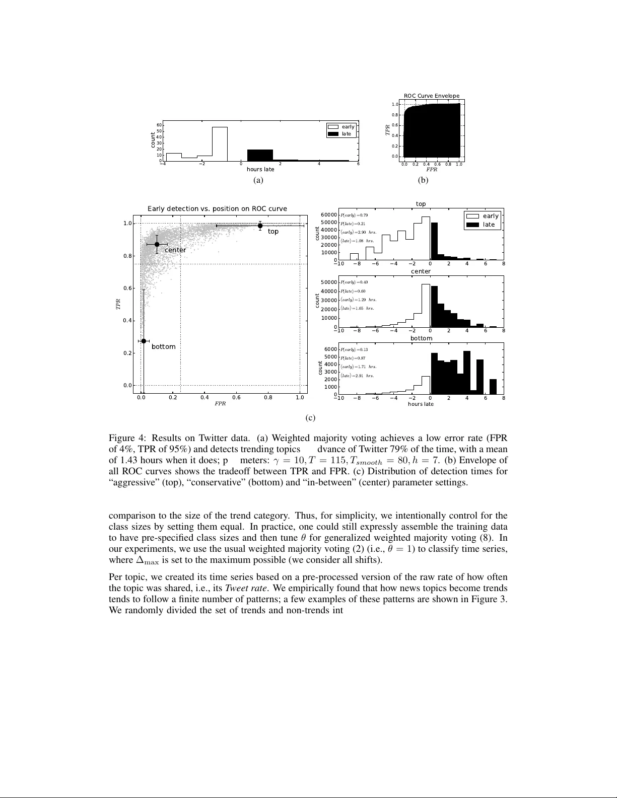
A Latent Sour ce Model f or Nonparametric T ime Series Classification George H. Chen MIT georgehc@mit.edu Stanislav Nik olov T witter snikolov@twitter.com Deva vrat Shah MIT devavrat@mit.edu Abstract For classifying time series, a nearest-neighbor approach is widely used in practice with performance often competitiv e with or better than more elaborate methods such as neural netw orks, decision trees, and support v ector machines. W e de velop theoretical justification for the ef fectiv eness of nearest-neighbor-lik e classifica- tion of time series. Our guiding hypothesis is that in many applications, such as forecasting which topics will become trends on T witter, there aren’t actually that many prototypical time series to begin with, relati v e to the number of time series we ha ve access to, e.g., topics become trends on T witter only in a fe w distinct man- ners whereas we can collect massive amounts of T witter data. T o operationalize this hypothesis, we propose a latent sour ce model for time series, which naturally leads to a “weighted majority voting” classification rule that can be approximated by a nearest-neighbor classifier . W e establish nonasymptotic performance guar- antees of both weighted majority voting and nearest-neighbor classification under our model accounting for how much of the time series we observ e and the model complexity . Experimental results on synthetic data sho w weighted majority voting achieving the same misclassification rate as nearest-neighbor classification while observing less of the time series. W e then use weighted majority to forecast which news topics on T witter become trends, where we are able to detect such “trending topics” in advance of T witter 79% of the time, with a mean early advantage of 1 hour and 26 minutes, a true positiv e rate of 95%, and a false positi v e rate of 4%. 1 Introduction Recent years ha ve seen an explosion in the av ailability of time series data related to virtually ev ery human endea vor — data that demands to be analyzed and turned into valuable insights. A key recurring task in mining this data is being able to classify a time series. As a running example used throughout this paper , consider a time series that tracks ho w much acti vity there is for a particular news topic on T witter . Giv en this time series up to present time, we ask “will this news topic go viral?” Borro wing T witter’ s terminology , we label the time series a “trend” and call its corresponding news topic a trending topic if the ne ws topic goes viral; otherwise, the time series has label “not trend”. W e seek to forecast whether a ne ws topic will become a trend befor e it is declared a trend (or not) by T witter , amounting to a binary classification problem. Importantly , we skirt the discussion of what makes a topic considered trending as this is irrelev ant to our mathematical dev elopment. 1 Furthermore, we remark that handling the case where a single time series can have different labels at different times is be yond the scope of this paper . 1 While it is not public knowledge how T witter defines a topic to be a trending topic, T witter does provide information for which topics are trending topics. W e take these labels to be ground truth, ef fectiv ely treating how a topic goes viral to be a black box supplied by T witter . 1 Numerous standard classification methods have been tailored to classify time series, yet a simple nearest-neighbor approach is hard to beat in terms of classification performance on a variety of datasets [22], with results competitiv e to or better than v arious other more elaborate methods such as neural networks [17], decision trees [18], and support vector machines [21]. More recently , researchers hav e examined which distance to use with nearest-neighbor classification [3, 8, 20] or how to boost classification performance by applying different transformations to the time series before using nearest-neighbor classification [2]. These existing results are mostly experimental, lacking theoretical justification for both when nearest-neighbor-lik e time series classifiers should be expected to perform well and ho w well. If we don’t confine ourselves to classifying time series, then as the amount of data tends to infinity , nearest-neighbor classification has been shown to achiev e a probability of error that is at worst twice the Bayes error rate, and when considering the nearest k neighbors with k allowed to grow with the amount of data, then the error rate approaches the Bayes error rate [6]. Howe v er , rather than examining the asymptotic case where the amount of data goes to infinity , we instead pursue nonasymptotic performance guarantees in terms of how lar ge of a training dataset we ha ve and ho w much we observe of the time series to be classified. T o arriv e at these nonasymptotic guarantees, we impose a low-comple xity structure on time series. Our contributions. W e present a model for which nearest-neighbor-l ike classification performs well by operationalizing the following hypothesis: In many time series applications, t here are only a small number of prot otypical time series relati ve to the number of time series we can collect. For e xample, posts on T witter are generated by humans, who are often beha viorally predictable in aggregate. This suggests that topics they post about only become trends on T witter in a few distinct manners, yet we hav e at our disposal enormous volumes of T witter data. In this context, we present a novel latent sour ce model : time series are generated from a small collection of m unknown latent sources, each having one of two labels, say “trend” or “not trend”. Our model’ s maximum a posteriori (MAP) time series classifier can be approximated by weighted majority voting, which compares the time series to be classified with each of the time series in the labeled training data. Each training time series casts a weighted vote in fav or of its ground truth label, with the weight depending on ho w similar the time series being classified is to the training example. The final classification is “trend” or “not trend” depending on which label has the higher ov erall vote. The voting is nonparametric in that it does not learn parameters for a model and is dri ven entirely by the training data. The unkno wn latent sources are nev er estimated; the training data serve as a proxy for these latent sources. W eighted majority voting itself can be approximated by a nearest-neighbor classifier , which we also analyze. Under our model, we sho w sufficient conditions so that if we hav e n = Θ( m log m δ ) time series in our training data, then weighted majority voting and nearest-neighbor classification correctly clas- sify a ne w time series with probability at least 1 − δ after observing its first Ω(log m δ ) time steps. As our analysis accounts for how much of the time series we observe, our results readily apply to the “online” setting in which a time series is to be classified while it streams in (as is the case for fore- casting trending topics) as well as the “of fline” setting where we hav e access to the entire time series. Also, while our analysis yields matching error upper bounds for the two classifiers, experimental re- sults on synthetic data suggests that weighted majority v oting outperforms nearest-neighbor classifi- cation early on when we observ e v ery little of the time series to be classified. Meanwhile, a specific instantiation of our model leads to a spherical Gaussian mixture model, where the latent sources are Gaussian mixture components. W e sho w that e xisting performance guarantees on learning spherical Gaussian mixture models [7, 11, 19] require more stringent conditions than what our results need, suggesting that learning the latent sources is ov erkill if the goal is classification. Lastly , we apply weighted majority v oting to forecasting trending topics on T witter . W e emphasize that our goal is pr ecognition of trends: predicting whether a topic is going to be a trend before it is actually declared to be a trend by T witter or , in theory , any other third party that we can collect ground truth labels from. Existing work that identify trends on T witter [4, 5, 15] instead, as part of their trend detection, define models for what trends are, which we do not do, nor do we assume we hav e access to such definitions. (The same could be said of previous work on novel document detection on T witter [12, 13].) In our experiments, weighted majority voting is able to predict whether a topic will be a trend in advance of T witter 79% of the time, with a mean early advantage of 1 hour and 26 minutes, a true positi ve rate of 95%, and a false positi ve rate of 4%. W e empirically find that the T witter activity of a news topic that becomes a trend tends to follow one of a finite number of patterns, which could be thought of as latent sources. 2 Outline. W eighted majority voting and nearest-neighbor classification for time series are pre- sented in Section 2. W e provide our latent source model and theoretical performance guarantees of weighted majority voting and nearest-neighbor classification under this model in Section 3. Ex- perimental results for synthetic data and forecasting trending topics on T witter are in Section 4. 2 W eighted Majority V oting and Nearest-Neighbor Classification Giv en a time-series 2 s : Z → R , we want to classify it as having either label +1 (“trend”) or − 1 (“not trend”). T o do so, we have access to labeled training data R + and R − , which denote the sets of all training time series with labels +1 and − 1 respectively . W eighted majority voting . Each positi vely-labeled example r ∈ R + casts a weighted vote e − γ d ( T ) ( r,s ) for whether time series s has label +1 , where d ( T ) ( r , s ) is some measure of similar- ity between the two time series r and s , superscript ( T ) indicates that we are only allo wed to look at the first T time steps (i.e., time steps 1 , 2 , . . . , T ) of s (but we’ re allowed to look outside of these time steps for the training time series r ), and constant γ ≥ 0 is a scaling parameter that determines the “sphere of influence” of each example. Similarly , each negati v ely-labeled example in R − also casts a weighted vote for whether time series s has label − 1 . The similarity measure d ( T ) ( r , s ) could, for example, be squared Euclidean distance: d ( T ) ( r , s ) = P T t =1 ( r ( t ) − s ( t )) 2 , k r − s k 2 T . Howe ver , this similarity measure only looks at the first T time steps of training time series r . Since time series in our training data are known, we need not restrict our attention to their first T time steps. Thus, we use the following similarity measure: d ( T ) ( r , s ) = min ∆ ∈{− ∆ max ,..., 0 ,..., ∆ max } T X t =1 ( r ( t + ∆) − s ( t )) 2 = min ∆ ∈{− ∆ max ,..., 0 ,..., ∆ max } k r ∗ ∆ − s k 2 T , (1) where we minimize ov er integer time shifts with a pre-specified maximum allo wed shift ∆ max ≥ 0 . Here, we have used q ∗ ∆ to denote time series q advanced by ∆ time steps, i.e., ( q ∗ ∆)( t ) = q ( t + ∆) . Finally , we sum up all of the weighted +1 votes and then all of the weighted − 1 votes. The label with the majority of ov erall weighted votes is declared as the label for s : b L ( T ) ( s ; γ ) = ( +1 if P r ∈R + e − γ d ( T ) ( r,s ) ≥ P r ∈R − e − γ d ( T ) ( r,s ) , − 1 otherwise . (2) Using a larger time windo w size T corresponds to waiting longer before we make a prediction. W e need to trade of f how long we wait and ho w accurate we want our prediction. Note that k - nearest-neighbor classification corresponds to only considering the k nearest neighbors of s among all training time series; all other votes are set to 0. W ith k = 1 , we obtain the follo wing classifier: Nearest-neighbor classifier . Let b r = arg min r ∈R + ∪R − d ( T ) ( r , s ) be the nearest neighbor of s . Then we declare the label for s to be: b L ( T ) N N ( s ) =  +1 if b r ∈ R + , − 1 if b r ∈ R − . (3) 3 A Latent Source Model and Theor etical Guarantees W e assume there to be m unkno wn latent sources (time series) that generate observed time series. Let V denote the set of all such latent sources; each latent source v : Z → R in V has a true label +1 or − 1 . Let V + ⊂ V be the set of latent sources with label +1 , and V − ⊂ V be the set of those with label − 1 . The observed time series are generated from latent sources as follo ws: 1. Sample latent source V from V uniformly at random. 3 Let L ∈ {± 1 } be the label of V . 2 W e index time using Z for notationally con venience b ut will assume time series to start at time step 1. 3 While we keep the sampling uniform for clarity of presentation, our theoretical guarantees can easily be extended to the case where the sampling is not uniform. The only change is that the number of training data needed will be larger by a factor of 1 mπ min , where π min is the smallest probability of a particular latent source occurring. 3 time a ctivi ty +1 { 1 +1 { 1 +1 { 1 Figure 1: Example of latent sources superimposed, where each latent source is shifted vertically in amplitude such that ev ery other latent source has label +1 and the rest have label − 1 . 2. Sample integer time shift ∆ uniformly from { 0 , 1 , . . . , ∆ max } . 3. Output time series S : Z → R to be latent source V advanced by ∆ time steps, followed by adding noise signal E : Z → R , i.e., S ( t ) = V ( t + ∆) + E ( t ) . The label associated with the generated time series S is the same as that of V , i.e., L . Entries of noise E are i.i.d. zero-mean sub-Gaussian with parameter σ , which means that for any time inde x t , E [exp( λE ( t ))] ≤ exp  1 2 λ 2 σ 2  for all λ ∈ R . (4) The f amily of sub-Gaussian distrib utions includes a v ariety of distrib utions, such as a zero- mean Gaussian with standard deviation σ and a uniform distrib ution over [ − σ , σ ] . The abov e generative process defines our latent source model. Importantly , we mak e no assumptions about the structure of the latent sources. For instance, the latent sources could be tiled as shown in Figure 1, where they are ev enly separated vertically and alternate between the two different classes +1 and − 1 . W ith a parametric model like a k -component Gaussian mixture model, estimating these latent sources could be problematic. For example, if we take any two adjacent latent sources with label +1 and cluster them, then this cluster could be confused with the latent source having label − 1 that is sandwiched in between. Noise only complicates estimating the latent sources. In this example, the k -component Gaussian mixture model needed for label +1 would require k to be the exact number of latent sources with label +1 , which is unknown. In general, the number of samples we need from a Gaussian mixture mixture model to estimate the mixture component means is exponential in the number of mixture components [16]. As we discuss next, for classification, we sidestep learning the latent sources altogether , instead using training data as a proxy for latent sources. At the end of this section, we compare our sample complexity for classification versus some existing sample comple xities for learning Gaussian mixture models. Classification. If we kne w the latent sources and if noise entries E ( t ) were i.i.d. N (0 , 1 2 γ ) across t , then the maximum a posteriori (MAP) estimate for label L gi ven an observ ed time series S = s is b L ( T ) MAP ( s ; γ ) = ( +1 if Λ ( T ) MAP ( s ; γ ) ≥ 1 , − 1 otherwise , (5) where Λ ( T ) MAP ( s ; γ ) , P v + ∈V + P ∆ + ∈D + exp  − γ k v + ∗ ∆ + − s k 2 T  P v − ∈V − P ∆ − ∈D + exp  − γ k v − ∗ ∆ − − s k 2 T  , (6) and D + , { 0 , . . . , ∆ max } . Howe v er , we do not know the latent sources, nor do we know if the noise is i.i.d. Gaussian. W e assume that we hav e access to training data as giv en in Section 2. W e make a further assumption that the training data were sampled from the latent source model and that we have n dif ferent training time series. Denote D , {− ∆ max , . . . , 0 , . . . , ∆ max } . Then we approximate the MAP classifier by using training data as a proxy for the latent sources. Specifically , we take ratio (6), replace the inner sum by a minimum in the exponent, replace V + and V − by R + and R − , and replace D + by D to obtain the ratio: Λ ( T ) ( s ; γ ) , P r + ∈R + exp  − γ  min ∆ + ∈D k r + ∗ ∆ + − s k 2 T  P r − ∈R − exp  − γ  min ∆ − ∈D k r − ∗ ∆ − − s k 2 T  . (7) 4 Plugging Λ ( T ) in place of Λ ( T ) MAP in classification rule (5) yields the weighted majority voting rule (2). Note that weighted majority v oting could be interpreted as a smoothed nearest-neighbor approxima- tion whereby we only consider the time-shifted version of each example time series that is closest to the observed time series s . If we didn’t replace the summations o ver time shifts with minimums in the exponent, then we hav e a kernel density estimate in the numerator and in the denominator [10, Chapter 7] (where the k ernel is Gaussian) and our main theoretical result for weighted majority voting to follo w would still hold using the same proof. 4 Lastly , applications may call for trading off true and false positi ve rates. W e can do this by general- izing decision rule (5) to declare the label of s to be +1 if Λ ( T ) ( s, γ ) ≥ θ and v ary parameter θ > 0 . The resulting decision rule, which we refer to as generalized weighted majority voting , is thus: b L ( T ) θ ( s ; γ ) =  +1 if Λ ( T ) ( s, γ ) ≥ θ , − 1 otherwise , (8) where setting θ = 1 recov ers the usual weighted majority voting (2). This modification to the classifier can be thought of as adjusting the priors on the relative sizes of the two classes. Our theoretical results to follow actually co ver this more general case rather than only that of θ = 1 . Theoretical guarantees. W e now present the main theoretical results of this paper which identify sufficient conditions under which generalized weighted majority voting (8) and nearest-neighbor classification (3) can classify a time series correctly with high probability , accounting for the size of the training dataset and how much we observe of the time series to be classified. First, we define the “gap” between R + and R − restricted to time length T and with maximum time shift ∆ max as: G ( T ) ( R + , R − , ∆ max ) , min r + ∈R + ,r − ∈R − , ∆ + , ∆ − ∈D k r + ∗ ∆ + − r − ∗ ∆ − k 2 T . (9) This quantity measures ho w far apart the two different classes are if we only look at length- T chunks of each time series and allow all shifts of at most ∆ max time steps in either direction. Our first main result is stated below . W e defer proofs for this section to Appendices A and B. Theorem 1. (P erformance guarantee for g eneralized weighted majority voting) Let m + = |V + | be the number of latent sour ces with label +1 , and m − = |V − | = m − m + be the number of latent sour ces with label − 1 . F or any β > 1 , under the latent sour ce model with n > β m log m time series in the training data, the pr obability of misclassifying time series S with label L using gener alized weighted majority voting b L ( T ) θ ( · ; γ ) satisfies the bound P ( b L ( T ) θ ( S ; γ ) 6 = L ) ≤  θ m + m + m − θ m  (2∆ max + 1) n exp  − ( γ − 4 σ 2 γ 2 ) G ( T ) ( R + , R − , ∆ max )  + m − β +1 . (10) An immediate consequence is that giv en error tolerance δ ∈ (0 , 1) and with choice γ ∈ (0 , 1 4 σ 2 ) , then upper bound (10) is at most δ (by having each of the two terms on the right-hand side be ≤ δ 2 ) if n > m log 2 m δ (i.e., β = 1 + log 2 δ / log m ), and G ( T ) ( R + , R − , ∆ max ) ≥ log( θm + m + m − θm ) + log (2∆ max + 1) + log n + log 2 δ γ − 4 σ 2 γ 2 . (11) This means that if we have access to a large enough pool of labeled time series, i.e., the pool has Ω( m log m δ ) time series, then we can subsample n = Θ( m log m δ ) of them to use as training data. Then with choice γ = 1 8 σ 2 , generalized weighted majority voting (8) correctly classifies a new time series S with probability at least 1 − δ if G ( T ) ( R + , R − , ∆ max ) = Ω  σ 2  log  θ m + m + m − θ m  + log(2∆ max + 1) + log m δ   . (12) Thus, the gap between sets R + and R − needs to gro w logarithmic in the number of latent sources m in order for weighted majority voting to classify correctly with high probability . Assuming that the 4 W e use a minimum rather a summation ov er time shifts to make the method more similar to existing time series classification work (e.g., [22]), which minimize ov er time warpings rather than simple shifts. 5 original unknown latent sources are separated (otherwise, there is no hope to distinguish between the classes using any classifier) and the gap in the training data grows as G ( T ) ( R + , R − , ∆ max ) = Ω( σ 2 T ) (otherwise, the closest two training time series from opposite classes are within noise of each other), then observing the first T = Ω(log( θ + 1 θ ) + log (2∆ max + 1) + log m δ ) time steps from the time series is sufficient to classify it correctly with probability at least 1 − δ . A similar result holds for the nearest-neighbor classifier (3). Theorem 2. (P erformance guarantee for near est-neighbor classification) F or any β > 1 , under the latent sour ce model with n > β m log m time series in the training data, the probability of misclassifying time series S with label L using the near est-neighbor classifier b L ( T ) N N ( · ) satisfies the bound P ( b L ( T ) N N ( S ) 6 = L ) ≤ (2∆ max + 1) n exp  − 1 16 σ 2 G ( T ) ( R + , R − , ∆ max )  + m − β +1 . (13) Our generalized weighted majority voting bound (10) with θ = 1 (corresponding to regular weighted majority voting) and γ = 1 8 σ 2 matches our nearest-neighbor classification bound, suggesting that the two methods have similar behavior when the gap grows with T . In practice, we find weighted majority voting to outperform nearest-neighbor classification when T is small, and then as T grows large, the two methods exhibit similar performance in agreement with our theoretical analysis. For small T , it could still be fairly likely that the nearest neighbor found has the wrong label, dooming the nearest-neighbor classifier to failure. W eighted majority voting, on the other hand, can recov er from this situation as there may be enough correctly labeled training time series close by that con- tribute to a higher overall vote for the correct class. This robustness of weighted majority v oting makes it fa v orable in the online setting where we want to make a prediction as early as possible. Sample complexity of learning the latent sources. If we can estimate the latent sources accurately , then we could plug these estimates in place of the true latent sources in the MAP classifier and achiev e classification performance close to optimal. If we restrict the noise to be Gaussian and assume ∆ max = 0 , then the latent source model corresponds to a spherical Gaussian mixture model. W e could learn such a model using Dasgupta and Schulman’ s modified EM algorithm [7]. Their theoretical guarantee depends on the true separation between the closest two latent sources, namely G ( T ) ∗ , min v ,v 0 ∈V s.t. v 6 = v 0 k v − v 0 k 2 2 , which needs to satisfy G ( T ) ∗  σ 2 √ T . Then with number of training time series n = Ω(max { 1 , σ 2 T G ( T ) ∗ } m log m δ ) , gap G ( T ) ∗ = Ω( σ 2 log m ε ) , and number of initial time steps observed T = Ω  max  1 , σ 4 T 2 ( G ( T ) ∗ ) 2  log  m δ max  1 , σ 4 T 2 ( G ( T ) ∗ ) 2  , (14) their algorithm achiev es, with probability at least 1 − δ , an additiv e εσ √ T error (in Euclidean distance) close to optimal in estimating e very latent source. In contrast, our result is in terms of gap G ( T ) ( R + , R − , ∆ max ) that depends not on the true separation between two latent sources but instead on the minimum observ ed separation in the training data between two time series of opposite labels. In fact, our gap, in their setting, gro ws as Ω( σ 2 T ) e v en when their gap G ( T ) ∗ grows sublinear in T . In particular, while their result cannot handle the regime where O ( σ 2 log m δ ) ≤ G ( T ) ∗ ≤ σ 2 √ T , ours can, using n = Θ( m log m δ ) training time series and observing the first T = Ω(log m δ ) time steps to classify a time series correctly with probability at least 1 − δ ; see Appendix D for details. V empala and W ang [19] ha ve a spectral method for learning Gaussian mixture models that can han- dle smaller G ( T ) ∗ than Dasgupta and Schulman’ s approach b ut requires n = e Ω( T 3 m 2 ) training data, where we’ ve hidden the dependence on σ 2 and other v ariables of interest for clarity of presentation. Hsu and Kakade [11] hav e a moment-based estimator that doesn’t ha ve a gap condition b ut, under a different non-degeneracy condition, requires substantially more samples for our problem setup, i.e., n = Ω(( m 14 + T m 11 ) /ε 2 ) to achie ve an ε approximation of the mixture components. These results need substantially more training data than what we’ v e sho wn is sufficient for classification. T o fit a Gaussian mixture model to massiv e training datasets, in practice, using all the training data could be prohibitiv ely expensi ve. In such scenarios, one could instead non-uniformly subsample O ( T m 3 /ε 2 ) time series from the training data using the procedure giv en in [9] and then feed the resulting smaller dataset, referred to as an ( m, ε ) - cor eset , to the EM algorithm for learning the latent sources. This procedure still requires more training time series than needed for classification and lacks a guarantee that the estimated latent sources will be close to the true latent sources. 6 0 50 100 150 200 0 0.1 0.2 0.3 0.4 0.5 0.6 T Classification error rate on test data Weighted majority voting Nearest−neighbor classifier Oracle MAP classifier (a) 1 2 3 4 5 6 7 8 0 0.05 0.1 0.15 0.2 0.25 β Classification error rate on test data Weighted majority voting Nearest−neighbor classifier Oracle MAP classifier (b) Figure 2: Results on synthetic data. (a) Classification error rate vs. number of initial time steps T used; training set size: n = β m log m where β = 8 . (b) Classification error rate at T = 100 vs. β . All experiments were repeated 20 times with newly generated latent sources, training data, and test data each time. Error bars denote one standard deviation abo ve and belo w the mean v alue. time activi ty Figure 3: Ho w ne ws topics become trends on T witter . The top left shows some time series of activity leading up to a ne ws topic becoming trending. These time series superimposed look like clutter , b ut we can separate them into different clusters, as shown in the next fi ve plots. Each cluster represents a “way” that a ne ws topic becomes trending. 4 Experimental Results Synthetic data. W e generate m = 200 latent sources, where each latent source is constructed by first sampling i.i.d. N (0 , 100) entries per time step and then applying a 1D Gaussian smoothing filter with scale parameter 30. Half of the latent sources are labeled +1 and the other half − 1 . Then n = β m log m training time series are sampled as per the latent source model where the noise added is i.i.d. N (0 , 1) and ∆ max = 100 . W e similarly generate 1000 time series to use as test data. W e set γ = 1 / 8 for weighted majority voting. For β = 8 , we compare the classification error rates on test data for weighted majority voting, nearest-neighbor classification, and the MAP classifier with oracle access to the true latent sources as sho wn in Figure 2(a). W e see that weighted majority voting outperforms nearest-neighbor classification but as T grows large, the two methods’ performances con ver ge to that of the MAP classifier . Fixing T = 100 , we then compare the classification error rates of the three methods using varying amounts of training data, as shown in Figure 2(b); the oracle MAP classifier is also shown but does not actually depend on training data. W e see that as β increases, both weighted majority v oting and nearest-neighbor classification steadily improve in performance. For ecasting trending topics on twitter . W e provide only an ov erview of our T witter results here, deferring full details to Appendix E. W e sampled 500 examples of trends at random from a list of June 2012 news trends, and 500 examples of non-trends based on phrases appearing in user posts during the same month. As we do not know how T witter chooses what phrases are considered as candidate phrases for trending topics, it’ s unclear what the size of the non-trend category is in 7 − 4 − 2 0 2 4 6 h o u r s l a t e 0 1 0 2 0 3 0 4 0 5 0 6 0 c o u n t F P R = 0 . 04 , TP R = 0 . 95 , P ( e a r l y ) = 0 . 79 ,  e a r l y  = 1 . 43 h r s γ = 10 , N o b s = 115 , N s m o o t h = 80 , h = 7 e a r l y l a t e (a) 0 . 0 0 . 2 0 . 4 0 . 6 0 . 8 1 . 0 F P R 0 . 0 0 . 2 0 . 4 0 . 6 0 . 8 1 . 0 TP R R O C C u r v e E n v e l o p e (b) 0 . 0 0 . 2 0 . 4 0 . 6 0 . 8 1 . 0 F P R 0 . 0 0 . 2 0 . 4 0 . 6 0 . 8 1 . 0 T P R t o p c e n t e r b o t t o m − 1 0 − 8 − 6 − 4 − 2 0 2 4 6 8 0 1 0 0 0 0 2 0 0 0 0 3 0 0 0 0 4 0 0 0 0 5 0 0 0 0 6 0 0 0 0 c o u n t P ( e a r l y ) = 0 . 79 P ( l a t e ) = 0 . 21  e a r l y  = 2 . 90 h r s .  l a t e  = 1 . 08 h r s . t o p e a r l y l a t e − 1 0 − 8 − 6 − 4 − 2 0 2 4 6 8 0 1 0 0 0 0 2 0 0 0 0 3 0 0 0 0 4 0 0 0 0 5 0 0 0 0 c o u n t P ( e a r l y ) = 0 . 40 P ( l a t e ) = 0 . 60  e a r l y  = 1 . 29 h r s .  l a t e  = 1 . 65 h r s . c e n t e r − 1 0 − 8 − 6 − 4 − 2 0 2 4 6 8 h o u r s l a t e 0 1 0 0 0 2 0 0 0 3 0 0 0 4 0 0 0 5 0 0 0 6 0 0 0 c o u n t P ( e a r l y ) = 0 . 13 P ( l a t e ) = 0 . 87  e a r l y  = 1 . 71 h r s .  l a t e  = 2 . 91 h r s . b o t t o m E a r l y d e t e c t i o n v s. p o si t i o n o n R O C c u r v e 0 . 0 0 . 2 0 . 4 0 . 6 0 . 8 1 . 0 F P R 0 . 0 0 . 2 0 . 4 0 . 6 0 . 8 1 . 0 T P R t o p c e n t e r b o t t o m − 1 0 − 8 − 6 − 4 − 2 0 2 4 6 8 0 1 0 0 0 0 2 0 0 0 0 3 0 0 0 0 4 0 0 0 0 5 0 0 0 0 6 0 0 0 0 c o u n t P ( e a r l y ) = 0 . 79 P ( l a t e ) = 0 . 21  e a r l y  = 2 . 90 h r s .  l a t e  = 1 . 08 h r s . t o p e a r l y l a t e − 1 0 − 8 − 6 − 4 − 2 0 2 4 6 8 0 1 0 0 0 0 2 0 0 0 0 3 0 0 0 0 4 0 0 0 0 5 0 0 0 0 c o u n t P ( e a r l y ) = 0 . 40 P ( l a t e ) = 0 . 60  e a r l y  = 1 . 29 h r s .  l a t e  = 1 . 65 h r s . c e n t e r − 1 0 − 8 − 6 − 4 − 2 0 2 4 6 8 h o u r s l a t e 0 1 0 0 0 2 0 0 0 3 0 0 0 4 0 0 0 5 0 0 0 6 0 0 0 c o u n t P ( e a r l y ) = 0 . 13 P ( l a t e ) = 0 . 87  e a r l y  = 1 . 71 h r s .  l a t e  = 2 . 91 h r s . b o t t o m E a r l y d e t e c t i o n v s. p o si t i o n o n R O C c u r v e (c) Figure 4: Results on T witter data. (a) W eighted majority voting achie ves a low error rate (FPR of 4%, TPR of 95%) and detects trending topics in adv ance of T witter 79% of the time, with a mean of 1.43 hours when it does; parameters: γ = 10 , T = 115 , T smooth = 80 , h = 7 . (b) En velope of all R OC curves shows the tradeoff between TPR and FPR. (c) Distribution of detection times for “aggressiv e” (top), “conserv ati ve” (bottom) and “in-between” (center) parameter settings. comparison to the size of the trend category . Thus, for simplicity , we intentionally control for the class sizes by setting them equal. In practice, one could still expressly assemble the training data to have pre-specified class sizes and then tune θ for generalized weighted majority voting (8). In our experiments, we use the usual weighted majority v oting (2) (i.e., θ = 1 ) to classify time series, where ∆ max is set to the maximum possible (we consider all shifts). Per topic, we created its time series based on a pre-processed version of the raw rate of how often the topic was shared, i.e., its T weet r ate . W e empirically found that how ne ws topics become trends tends to follow a finite number of patterns; a fe w examples of these patterns are shown in Figure 3. W e randomly divided the set of trends and non-trends into into two halves, one to use as training data and one to use as test data. W e applied weighted majority voting, sweeping ov er γ , T , and data pre-processing parameters. As shown in Figure 4(a), one choice of parameters allo ws us to detect trending topics in advance of T witter 79% of the time, and when we do, we detect them an av erage of 1.43 hours earlier . Furthermore, we achie ve a true positi ve rate (TPR) of 95% and a false positiv e rate (FPR) of 4%. Naturally , there are tradeoffs between TPR, FPR, and ho w early we make a prediction (i.e., ho w small T is). As sho wn in Figure 4(c), an “aggressi ve” parameter setting yields early detection and high TPR but high FPR, and a “conservati ve” parameter setting yields low FPR but late detection and lo w TPR. An “in-between” setting can strike the right balance. Acknowledgements. This work was supported in part by the Army Research Office under MURI A ward 58153-MA-MUR. GHC w as supported by an NDSEG fello wship. 8 References [1] Sitaram Asur , Bernardo A. Huberman, G ´ abor Szab ´ o, and Chunyan W ang. Trends in social media: Per- sistence and decay . In Proceedings of the F ifth International Confer ence on W eblogs and Social Media , 2011. [2] Anthony Bagnall, Luke Davis, Jon Hills, and Jason Lines. Transformation based ensembles for time series classification. In Pr oceedings of the 12th SIAM International Confer ence on Data Mining , pages 307–319, 2012. [3] Gustav o E.A.P .A. Batista, Xiaoyue W ang, and Eamonn J. Keogh. A complexity-in v ariant distance mea- sure for time series. In Pr oceedings of the 11th SIAM International Conference on Data Mining , pages 699–710, 2011. [4] Hila Becker , Mor Naaman, and Luis Grav ano. Beyond trending topics: Real-world event identification on Twitter . In Pr oceedings of the F ifth International Confer ence on W eblogs and Social Media , 2011. [5] Mario Cataldi, Luigi Di Caro, and Claudio Schifanella. Emerging topic detection on twitter based on temporal and social terms evaluation. In Pr oceedings of the 10th International W orkshop on Multimedia Data Mining , 2010. [6] Thomas M. Cover and Peter E. Hart. Nearest neighbor pattern classification. IEEE T ransactions on Information Theory , 13(1):21–27, 1967. [7] Sanjoy Dasgupta and Leonard Schulman. A probabilistic analysis of EM for mixtures of separated, spherical gaussians. Journal of Machine Learning Resear c h , 8:203–226, 2007. [8] Hui Ding, Goce Trajce vski, Peter Scheuermann, Xiaoyue W ang, and Eamonn K eogh. Querying and min- ing of time series data: experimental comparison of representations and distance measures. Proceedings of the VLDB Endowment , 1(2):1542–1552, 2008. [9] Dan Feldman, Matthew F aulkner , and Andreas Krause. Scalable training of mixture models via coresets. In Advances in Neural Information Pr ocessing Systems 24 , 2011. [10] Keinosuk e Fukunaga. Introduction to statistical pattern recognition (2nd ed.) . Academic Press Profes- sional, Inc., 1990. [11] Daniel Hsu and Sham M. Kakade. Learning mixtures of spherical gaussians: Moment methods and spectral decompositions, 2013. [12] Shiv a Prasad Kasiviswanathan, Prem Melville, Arindam Banerjee, and V ikas Sindhwani. Emerging topic detection using dictionary learning. In Pr oceedings of the 20th ACM Confer ence on Information and Knowledge Manag ement , pages 745–754, 2011. [13] Shiv a Prasad Kasi viswanathan, Huahua W ang, Arindam Banerjee, and Prem Melville. Online l1- dictionary learning with application to novel document detection. In Advances in Neural Information Pr ocessing Systems 25 , pages 2267–2275, 2012. [14] Beatrice Laurent and Pascal Massart. Adapti ve estimation of a quadratic functional by model selection. Annals of Statistics , 28(5):1302–1338, 2000. [15] Michael Mathioudakis and Nick Koudas. T wittermonitor: trend detection ov er the Twitter stream. In Pr oceedings of the 2010 A CM SIGMOD International Confer ence on Manag ement of Data , 2010. [16] Ankur Moitra and Gre gory V aliant. Settling the polynomial learnability of mixtures of gaussians. In 51st Annual IEEE Symposium on F oundations of Computer Science , pages 93–102, 2010. [17] Alex Nanopoulos, Rob Alcock, and Y annis Manolopoulos. Feature-based classification of time-series data. International Journal of Computer Resear ch , 10, 2001. [18] Juan J. Rodr ´ ıguez and Carlos J. Alonso. Interval and dynamic time warping-based decision trees. In Pr oceedings of the 2004 A CM Symposium on Applied Computing , 2004. [19] Santosh V empala and Grant W ang. A spectral algorithm for learning mixture models. Journal of Com- puter and System Sciences , 68(4):841–860, 2004. [20] Kilian Q. W einber ger and Lawrence K. Saul. Distance metric learning for lar ge margin nearest neighbor classification. Journal of Machine Learning Resear c h , 10:207–244, 2009. [21] Y i W u and Edward Y . Chang. Distance-function design and fusion for sequence data. In Proceedings of the 2004 A CM International Confer ence on Information and Knowledge Management , 2004. [22] Xiaopeng Xi, Eamonn J. K eogh, Christian R. Shelton, Li W ei, and Chotirat Ann Ratanamahatana. F ast time series classification using numerosity reduction. In Pr oceedings of the 23rd International Confer ence on Machine Learning , 2006. 9 A Proof of Theor em 1 Let S be the time series with an unknown label that we wish to classify using training data. Denote m + , |V + | , m − , |V − | = m − m + , n + , |R + | , n − , |R − | , and R , R + ∪ R − . Recall that D + , { 0 , 1 , . . . , ∆ max } , and D , {− ∆ max , . . . , − 1 , 0 , 1 , . . . , ∆ max } . As per the model, there exists a latent source V , shift ∆ 0 ∈ D + , and noise signal E 0 such that S = V ∗ ∆ 0 + E 0 . (15) Applying a standard coupon collector’ s problem result, with a training set of size n > β m log m , then with probability at least 1 − m − β +1 , for each latent source V ∈ V , there e xists at least one time series R in the set R of all training data that is generated from V . Henceforth, we assume that this ev ent holds. In Appendix C, we elaborate on what happens if the latent sources are not uniformly sampled. Note that R is generated from V as R = V ∗ ∆ 00 + E 00 , (16) where ∆ 00 ∈ D + and E 00 is a noise signal independent of E 0 . Therefore, we can re write S in terms of R as follo ws: S = R ∗ ∆ + E , (17) where ∆ = ∆ 0 − ∆ 00 ∈ D (note the change from D + to D ) and E = E 0 − E 00 ∗ ∆ . Since E 0 and E 00 are i.i.d. o ver time and sub-Gaussian with parameter σ , one can easily v erify that E is i.i.d. over time and sub-Gaussian with parameter √ 2 σ . W e no w bound the probability of error of classifier b L ( T ) θ ( · ; γ ) . The probability of error or misclassi- fication using the first T time steps of S is giv en by P  misclassify S using its first T time steps  = P ( b L ( T ) θ ( S ; γ ) = − 1 | L = +1) P ( L = +1) | {z } m + /m + P ( b L ( T ) θ ( S ; γ ) = +1 | L = − 1) P ( L = − 1) | {z } m − /m . (18) In the remainder of the proof, we primarily show ho w to bound P ( b L ( T ) θ ( S ; γ ) = − 1 | L = +1) . The bound for P ( b L ( T ) θ ( S ; γ ) = +1 | L = − 1) is almost identical. By Marko v’ s inequality , P ( b L ( T ) θ ( S ; γ ) = − 1 | L = +1) = P  1 Λ ( T ) ( S ; γ ) ≥ 1 θ    L = +1  ≤ θ E  1 Λ ( T ) ( S ; γ )    L = +1  . (19) Now , E  1 Λ ( T ) ( S ; γ )    L = +1  ≤ max r + ∈R + , ∆ + ∈D E E  1 Λ ( T ) ( r + ∗ ∆ + + E ; γ )  . (20) W ith the above inequality in mind, we next bound 1 / Λ ( T ) ( e r + ∗ e ∆ + + E ; γ ) for any choice of e r + ∈ R + and e ∆ + ∈ D . Note that for any time series s , 1 Λ ( T ) ( s ; γ ) ≤ P r − ∈R − , ∆ − ∈D exp  − γ k r − ∗ ∆ − − s k 2 T  exp  − γ k e r + ∗ e ∆ + − s k 2 T  . (21) After ev aluating the abo ve for s = e r + ∗ e ∆ + + E , a bit of algebra shows that 1 Λ ( T ) ( e r + ∗ e ∆ + + E ; γ ) ≤ X r − ∈R − , ∆ − ∈D  exp  − γ k e r + ∗ e ∆ + − r − ∗ ∆ − k 2 T  exp  − 2 γ h e r + ∗ e ∆ + − r − ∗ ∆ − , E i T  , (22) where h q , q 0 i T , P T t =1 q ( t ) q 0 ( t ) for time series q and q 0 . 10 T aking the expectation of (22) with respect to noise signal E , we obtain the follo wing bound: E E  1 Λ ( T ) ( e r + ∗ e ∆ + + E ; γ )  ≤ E E  X r − ∈R − , ∆ − ∈D n exp  − γ k e r + ∗ e ∆ + − r − ∗ ∆ − k 2 T  exp  − 2 γ h e r + ∗ e ∆ + − r − ∗ ∆ − , E i T  o  ( i ) = X r − ∈R − , ∆ − ∈D exp  − γ k e r + ∗ e ∆ + − r − ∗ ∆ − k 2 T  T Y t =1 E E ( t ) [exp  − 2 γ ( e r + ( t + e ∆ + ) − r − ( t + ∆ − )) E ( t )  ] ( ii ) ≤ X r − ∈R − , ∆ − ∈D exp  − γ k e r + ∗ e ∆ + − r − ∗ ∆ − k 2 T  T Y t =1 exp  4 σ 2 γ 2 ( e r + ( t + e ∆ + ) − r − ( t + ∆ − )) 2  = X r − ∈R − , ∆ − ∈D exp  − ( γ − 4 σ 2 γ 2 ) k r + ∗ ∆ + − r − ∗ ∆ − k 2 T  ≤ (2∆ max + 1) n − exp  − ( γ − 4 σ 2 γ 2 ) G ( T )  , (23) where step ( i ) uses independence of entries of E , step ( ii ) uses the f act that E ( t ) is zero-mean sub- Gaussian with parameter √ 2 σ , and the last line abbre viates the gap G ( T ) ≡ G ( T ) ( R + , R − , ∆ max ) . Stringing together inequalities (19), (20), and (23), we obtain P ( b L ( T ) θ ( S ; γ ) = − 1 | L = +1) ≤ θ (2∆ max + 1) n − exp  − ( γ − 4 σ 2 γ 2 ) G ( T )  . (24) Repeating a similar argument yields P ( b L ( T ) θ ( S ; γ ) = +1 | L = − 1) ≤ 1 θ (2∆ max + 1) n + exp  − ( γ − 4 σ 2 γ 2 ) G ( T )  . (25) Finally , plugging (24) and (25) into (18) gives P ( b L ( T ) θ ( S ; γ ) 6 = L ) ≤ θ (2∆ max + 1) n − m + m exp  − ( γ − 4 σ 2 γ 2 ) G ( T )  + 1 θ (2∆ max + 1) n + m − m (2∆ max + 1) n + exp  − ( γ − 4 σ 2 γ 2 ) G ( T )  =  θ m + m + m − θ m  (2∆ max + 1) n exp  − ( γ − 4 σ 2 γ 2 ) G ( T )  . (26) This completes the proof of Theorem 1. B Proof of Theor em 2 The proof uses similar steps as the weighted majority voting case. As before, we consider the case when our training data sees each latent source at least once (this e vent happens with probability at least 1 − m − β +1 ). W e decompose the probability of error into terms depending on which latent source V generated S : P ( b L ( T ) N N ( S ) 6 = L ) = X v ∈V P ( V = v ) P ( b L ( T ) N N ( S ) 6 = L | V = v ) = X v ∈V 1 m P ( b L ( T ) N N ( S ) 6 = L | V = v ) . (27) Next, we bound each P ( b L ( T ) N N ( S ) 6 = L | V = v ) term. Suppose that v ∈ V + , i.e., v has label L = +1 ; the case when v ∈ V − is similar . Then we make an error and declare b L ( T ) N N ( S ) = − 1 when the nearest neighbor b r to time series S is in the set R − , where ( b r , b ∆) = arg min ( r, ∆) ∈R×D k r ∗ ∆ − S k 2 T . (28) 11 By our assumption that e very latent source is seen in the training data, there exists r ∗ ∈ R + gener- ated by latent source v , and so S = r ∗ ∗ ∆ ∗ + E (29) for some shift ∆ ∗ ∈ D and noise signal E consisting of i.i.d. entries that are zero-mean sub-Gaussian with parameter √ 2 σ . By optimality of ( b r , b ∆) for optimization problem (28), we ha ve k r ∗ ∆ − ( r ∗ ∗ ∆ ∗ + E ) k 2 T ≥ k b r ∗ b ∆ − ( r ∗ ∗ ∆ ∗ + E ) k 2 T for all r ∈ R , ∆ ∈ D . (30) Plugging in r = r ∗ and ∆ = ∆ ∗ , we obtain k E k 2 T ≥ k b r ∗ b ∆ − ( r ∗ ∗ ∆ ∗ + E ) k 2 T = k ( b r ∗ b ∆ − r ∗ ∗ ∆ ∗ ) − E k 2 T = k b r ∗ b ∆ − r ∗ ∗ ∆ ∗ k 2 T − 2 h b r ∗ b ∆ − r ∗ ∗ ∆ ∗ , E i T + k E k 2 T , (31) or , equi v alently , 2 h b r ∗ b ∆ − r ∗ ∗ ∆ ∗ , E i T ≥ k b r ∗ b ∆ − r ∗ ∗ ∆ ∗ k 2 T . (32) Thus, gi ven V = v ∈ V + , declaring b L ( T ) N N ( S ) = − 1 implies the existence of b r ∈ R − and b ∆ ∈ D such that optimality condition (32) holds. Therefore, P ( b L ( T ) N N ( S ) = − 1 | V = v ) ≤ P  [ b r ∈R − , b ∆ ∈D { 2 h b r ∗ b ∆ − r ∗ ∗ ∆ ∗ , E i T ≥ k b r ∗ b ∆ − r ∗ ∗ ∆ ∗ k 2 T }  ( i ) ≤ (2∆ max + 1) n − P (2 h b r ∗ b ∆ − r ∗ ∗ ∆ ∗ , E i T ≥ k b r ∗ b ∆ − r ∗ ∗ ∆ ∗ k 2 T ) ≤ (2∆ max + 1) n − P (exp(2 λ h b r ∗ b ∆ − r ∗ ∗ ∆ ∗ , E i T ) ≥ exp( λ k b r ∗ b ∆ − r ∗ ∗ ∆ ∗ k 2 T )) ( ii ) ≤ (2∆ max + 1) n − exp( − λ k b r ∗ b ∆ − r ∗ ∗ ∆ ∗ k 2 T ) E [exp(2 λ h b r ∗ b ∆ − r ∗ ∗ ∆ ∗ , E i T )] ( iii ) ≤ (2∆ max + 1) n − exp( − λ k b r ∗ b ∆ − r ∗ ∗ ∆ ∗ k 2 T ) exp(4 λ 2 σ 2 k b r ∗ b ∆ − r ∗ ∗ ∆ ∗ k 2 T ) = (2∆ max + 1) n − exp( − ( λ − 4 λ 2 σ 2 ) k b r ∗ b ∆ − r ∗ ∗ ∆ ∗ k 2 T ) ≤ (2∆ max + 1) n exp( − ( λ − 4 λ 2 σ 2 ) G ( T ) ) ( iv ) ≤ (2∆ max + 1) n exp  − 1 16 σ 2 G ( T )  , (33) where step ( i ) is by a union bound, step ( ii ) is by Marko v’ s inequality , step ( iii ) is by sub- Gaussianity , and step ( iv ) is by choosing λ = 1 8 σ 2 . As bound (33) also holds for P ( b L ( T ) N N ( S ) = +1 | V = v ) when instead v ∈ V − , we can no w piece together (27) and (33) to yield the final result: P ( b L ( T ) N N ( S ) 6 = L ) = X v ∈V 1 m P ( b L ( T ) N N ( S ) 6 = L | V = v ) ≤ (2∆ max + 1) n exp  − 1 16 σ 2 G ( T )  . (34) C Handling Non-unif ormly Sampled Latent Sources When each time series generated from the latent source model is sampled uniformly at random, then having n > m log 2 m δ (i.e., β = 1 + log 2 δ / log m ) ensures that with probability at least 1 − δ 2 , our training data sees e very latent source at least once. When the latent sources aren’ t sampled uniformly at random, we show that we can simply replace the condition n > m log 2 m δ with n ≥ 8 π min log 2 m δ to achieve a similar (in fact, stronger) guarantee, where π min is the smallest probability of a particular latent source occurring. 12 Lemma 3. Suppose that the i -th latent sour ce occurs with pr obability π i in the latent sour ce model. Denote π min , min i ∈{ 1 , 2 ,...,m } π i . Let ξ i be the number of times that the i -th latent sour ce appears in the training data. If n ≥ 8 π min log 2 m δ , then with pr obability at least 1 − δ 2 , every latent sour ce appears strictly gr eater than 1 2 nπ min times in the training data. Pr oof. Note that ξ i ∼ Bin ( n, π i ) . W e have P  ξ i ≤ 1 2 nπ min  ≤ P  ξ i ≤ 1 2 nπ i  ( i ) ≤ exp  − 1 2 · ( nπ i − 1 2 nπ i ) 2 n · π i  = exp  − nπ i 8  ≤ exp  − nπ min 8  . (35) where step ( i ) uses a standard binomial distrib ution lower tail bound. Applying a union bound, P  [ i ∈{ 1 , 2 ,...,m }  ξ i ≤ 1 2 nπ min   ≤ m exp  − nπ min 8  , (36) which is at most δ 2 when n ≥ 8 π min log 2 m δ . D Sample Complexity f or the Gaussian Setting Without T ime Shifts Existing results on learning mixtures of Gaussians by Dasgupta and Schulman [7] and by V empala and W ang [19] use a different notion of gap than we do. In our notation, their gap can be written as G ( T ) ∗ , min v ,v 0 ∈V s.t. v 6 = v 0 k v − v 0 k 2 T , (37) which measures the minimum separation between the true latent sources, disregarding their labels. W e now translate our main theoretical guarantees to be in terms of gap G ( T ) ∗ under the assumption that the noise is Gaussian and that there are no time shifts. Theorem 4. Under the latent sour ce model, suppose that the noise is zer o-mean Gaussian with variance σ 2 , that ther e ar e no time shifts (i.e ., ∆ max = 0 ), and that we have sampled n > m log 4 m δ training time series. Then if G ( T ) ∗ ≥ 4 σ 2 log 4 n 2 δ , (38) T ≥ (12 + 8 √ 2) log 4 n 2 δ , (39) then weighted majority voting (with θ = 1 , γ = 1 8 σ 2 ) and nearest-neighbor classification each classify a new time series corr ectly with pr obability at least 1 − δ . In particular , with access to a pool of Ω( m log m δ ) time series, we can subsample n = Θ( m log m δ ) of them to use as training data. Then provided that G ( T ) ∗ = Ω( σ 2 log m δ ) and T = Ω(log m δ ) , we correctly classify a new time series with probability at least 1 − δ . Pr oof. The basic idea is to show that with high probability , our gap G ( T ) ≡ G ( T ) ( R + , R − , ∆ max ) satisfies G ( T ) ≥ G ( T ) ∗ + 2 σ 2 T − 4 σ r G ( T ) ∗ log 4 n 2 δ − 4 σ 2 r T log 4 n 2 δ . (40) The worst-case scenario occurs when G ( T ) ∗ = 4 σ 2 log 4 n 2 δ , at which point we hav e G ( T ) ≥ 2 σ 2 T − 4 σ 2 log 4 n 2 δ − 4 σ 2 r T log 4 n 2 δ . (41) 13 The right-hand side is at least σ 2 T when T ≥ (12 + 8 √ 2) log 4 n 2 δ , (42) which ensures that, with high probability , G ( T ) ≥ σ 2 T . Theorems 1 and 2 each say that if we further hav e n > m log 4 m δ , and T ≥ 16 log 4 n δ , then we classify a ne w time series correctly with high probability , where we note that T ≥ (12 + 8 √ 2) log 4 n 2 δ ≥ 16 log 4 n δ . W e now fill in the details. Let r + and r − be two time series in the training data that ha ve labels +1 and − 1 respectively , where we assume that ∆ max = 0 . Let v ( r + ) ∈ V and v ( r − ) ∈ V be the true latent sources of r + and r − , respectiv ely . This means that r + ∼ N ( v ( r + ) , σ 2 I T × T ) and r − ∼ N ( v ( r − ) , σ 2 I T × T ) . Denoting E ( r + ) ∼ N (0 , σ 2 I T × T ) and E ( r − ) ∼ N (0 , σ 2 I T × T ) to be noise associated with time series r + and r − , we hav e k r + − r − k 2 T = k ( v ( r + ) + E ( r + ) ) − ( v ( r − ) + E ( r − ) ) k 2 T = k v ( r + ) − v ( r − ) k 2 T + 2 h v ( r + ) − v ( r − ) , E ( r + ) − E ( r − ) i + k E ( r + ) − E ( r − ) k 2 T . (43) W e shall show that with high probability , for all r + ∈ R + and for all r − ∈ R − : h v ( r + ) − v ( r − ) , E ( r + ) − E ( r − ) i ≥ − 2 σ k v ( r + ) − v ( r − ) k T r log 4 n 2 δ , (44) k E ( r + ) − E ( r − ) k 2 T ≥ 2 σ 2 T − 4 σ 2 r T log 4 n 2 δ . (45) • Bound (44): h v ( r + ) − v ( r − ) , E ( r + ) − E ( r − ) i is zero-mean sub-Gaussian with parameter √ 2 σ k v ( r + ) − v ( r − ) k T , so P ( h v ( r + ) − v ( r − ) , E ( r + ) − E ( r − ) i ≤ − a ) ≤ exp  − a 2 4 σ 2 k v ( r + ) − v ( r − ) k 2 T  = δ 4 n 2 (46) with choice a = 2 σ k v ( r + ) − v ( r − ) k T q log 4 n 2 δ . A union bound ov er all pairs of time series in the training data with opposite labels giv es P [ r + ∈R + , r − ∈R −  h v ( r + ) − v ( r − ) , E ( r + ) − E ( r − ) i ≤ − 2 σ k v ( r + ) − v ( r − ) k T r log 4 n 2 δ  ! ≤ δ 4 . (47) • Bound (45): Due to a result by Laurent and Massart [14, Lemma 1], we have P ( k E ( r + ) − E ( r − ) k 2 T ≤ 2 σ 2 T − 4 σ 2 √ T a ) ≤ e − a = δ 4 n 2 (48) with choice a = log 4 n 2 δ . A union bound giv es P [ r + ∈R + , r − ∈R −  k E ( r + ) − E ( r − ) k 2 T ≤ 2 σ 2 T − 4 σ 2 r T log 4 n 2 δ  ! ≤ δ 4 . (49) Assuming that bounds (44) and (45) both hold, then for all r + ∈ R + , r − ∈ R − , we hav e k r + − r − k 2 T = k v ( r + ) − v ( r − ) k 2 T + 2 h v ( r + ) − v ( r − ) , E ( r + ) − E ( r − ) i + k E ( r + ) − E ( r − ) k 2 T ≥ k v ( r + ) − v ( r − ) k 2 T − 4 σ k v ( r + ) − v ( r − ) k T r log 4 n 2 δ + 2 σ 2 T − 4 σ 2 r T log 4 n 2 δ ( i ) =  k v ( r + ) − v ( r − ) k T − 2 σ r log 4 n 2 δ  2 − 4 σ 2 log 4 n 2 δ + 2 σ 2 T − 4 σ 2 r T log 4 n 2 δ ( ii ) ≥  p G ( T ) ∗ − 2 σ r log 4 n 2 δ  2 + 2 σ 2 T − 4 σ 2 log 4 n 2 δ − 4 σ 2 r T log 4 n 2 δ , (50) 14 where step ( i ) follows from completing the square, and step ( ii ) uses our assumption that G ( T ) ∗ ≥ 4 σ 2 log 4 n 2 δ . Minimizing over r + ∈ R + and r − ∈ R − , we get G ( T ) ≥  p G ( T ) ∗ − 2 σ r log 4 n 2 δ  2 + 2 σ 2 T − 4 σ 2 log 4 n 2 δ − 4 σ 2 r T log 4 n 2 δ . (51) The worst-case scenario occurs when G ( T ) ∗ = 4 σ 2 log 4 n 2 δ , in which case G ( T ) ≥ 2 σ 2 T − 4 σ 2 log 4 n 2 δ − 4 σ 2 r T log 4 n 2 δ . (52) Theorems 1 and 2 imply that having G ( T ) ≥ σ 2 T , n > m log 4 m δ , and T ≥ 16 log 4 n δ allows weighted majority voting (with θ = 1 , γ = 1 8 σ 2 ) and nearest-neighbor classification to each succeed with high probability . W e achieve G ( T ) ≥ σ 2 T by asking that 2 σ 2 T − 4 σ 2 log 4 n 2 δ − 4 σ 2 r T log 4 n 2 δ ≥ σ 2 T , (53) which happens when T ≥ (12 + 8 √ 2) log 4 n 2 δ . (54) A union bound over the following four bad ev ents (each controlled to happen with probability at most δ 4 ) yields the final result: • Not ev ery latent source is seen in the training data. • Bound (44) doesn’t hold. • Bound (45) doesn’t hold. • Assuming that the abov e three bad ev ents don’ t happen, we still misclassify . E F orecasting T rending T opics on T witter T witter is a social network whose users post messages called T weets , which are then broadcast to a user’ s followers. Often, emerging topics of interest are discussed on T witter in real time. Inevitably , certain topics gain sudden popularity and — in T witter speak — begin to tr end . T witter surfaces such topics as a list of top ten tr ending topics , or tr ends . Data. W e sampled 500 examples of trends at random from a list of June 2012 news trends and recorded the earliest time each topic trended within the month. Before sampling, we filtered out trends that ne ver achiev ed a rank of 3 or better on the T witter trends list 5 as well as trends that lasted for less than 30 minutes as to keep our trend examples reasonably salient. W e also sampled 500 examples of non-trends at random from a list of n -grams (of sizes 1, 2, and 3) appearing in T weets created in June 2012, where we filter out any n -gram containing words that appeared in one of our 500 chosen trend examples. Note that as we do not know how T witter chooses what phrases are considered as topic phrases (and are candidates for trending topics), it’ s unclear what the size of the non-trend category is in comparison to the size of the trend category . Thus, for simplicity , we intentionally control for the class sizes by setting them equal. In practice, one could still expressly assemble the training data to ha v e pre-specified class sizes and then tune θ for generalized weighted majority voting (8). In our experiments, we just use the usual weighted majority voting (2) (i.e., θ = 1 ) to classify time series. From these e xamples of trends and non-trends, we then created time series of acti vity for each topic based on the rate of T weets about that topic over time. T o approximate this rate, we gathered 10% of all T weets from June 2012, placed them into two-minute b uckets according to their timestamps, and counted the number of T weets in each bucket. W e denote the count at the t -th time b ucket as ρ ( t ) , which we refer to as the ra w rate. W e then transform the raw rate in a number of ways, summarized in Figure 5, before using the resulting time series for classification. 5 On T witter, trending topics compete for the top ten spots whereas we are only detecting whether a topic will trend or not. 15 ½ ( t ) ½ b ( t ) Ba s e li n e n o r m a li z a tio n Em p h a s ize la r g e s p ik e s ½ b , s ( t ) S m o o thi n g ½ b , s , c ( t ) Lo g ½ b , s , c , l ( t ) Figure 5: T witter data pre-processing pipeline: The raw rate ρ ( t ) counts the number of T weets in time bucket t . W e normalize ρ ( t ) to make the counts relativ e: ρ b ( t ) , ρ ( t ) / P t τ =1 ρ ( τ ) . Large spikes are emphasized: ρ b,s ( t ) , | ρ b ( t ) − ρ b ( t − 1) | α (we use α = 1 . 2 ). Next, we smooth the signal: ρ b,s,c ( t ) , P t τ = t − T smooth +1 ρ b,s ( τ ) . Finally , we take the log: ρ b,s,c,l ( t ) , log ρ b,s,c ( t ) . W e observed that trending activity is characterized by spikes above some baseline rate, whereas non-trending activity has fewer , if any spikes. For example, a non-trending topic such as “city” has a very high, but mostly constant rate because it is a common word. In contrast, soon-to-be-trending topics like “Miss USA ” will initially ha v e a low rate, b ut will also ha ve bursts in acti vity as the ne ws spreads. T o emphasize the parts of the rate signal abov e the baseline and de-emphasize the parts below the baseline, we define a baseline-normalized signal ρ b ( t ) , ρ ( t ) / P t τ =1 ρ ( τ ) . A related observ ation is that the T weet rate for a trending topic typically contains larger and more sudden spikes than those of non-trending topics. W e rew ard such spikes by emphasizing them, while de-emphasizing smaller spikes. T o do so, we define a baseline-and-spike-normalized rate ρ b,s ( t ) , | ρ b ( t ) − ρ b ( t − 1) | α in terms of the already baseline-normalized rate ρ b ; parameter α ≥ 1 controls ho w much spik es are re warded (we used α = 1 . 2 ). In addition, we con v olve the result with a smoothing window to eliminate noise and effecti vely measure the v olume of T weets in a sliding window of length T smooth : ρ b,s,c ( t ) , P t τ = t − T smooth +1 ρ b,s ( τ ) . Finally , the spread of a topic from person to person can be thought of as a branching process in which a population of users “affected” by a topic grows exponentially with time, with the exponent depending on the details of the model [1]. This intuition suggests using a logarithmic scaling for the volume of T weets: ρ b,s,c,l ( t ) , log ρ b,s,c ( t ) . The resulting time series ρ b,s,c,l contains data from the entire window in which data was collected. T o construct the sets of training time series R + and R − , we keep only a small h -hour slice of repre- sentativ e acti vity r for each topic. Namely , each of the final time series r used in the training data is truncated to only contain the h hours of acti vity in the corresponding transformed time series ρ b,s,c,l . For time series corresponding to trending topics, these h hours are taken from the time leading up to when the topic was first declared by T witter to be trending. For time series corresponding to non-trending topics, the h -hour windo w of acti vity is sampled at random from all the acti vity for the topic. W e empirically found that how news topics become trends tends to follow a finite number of patterns; a few e xamples of these patterns are sho wn in Figure 3. Experiment. For a fix ed choice of parameters, we randomly divided the set of trends and non-trends into tw o halv es, one for training and one for testing. W eighted majority v oting with the training data was used to classify the test data. Per time series in the test data, we looked within a window of 2 h hours, centered at the trend onset for trends, and sampled randomly for non-trends. W e restrict detection to this time window to av oid detecting earlier times that a topic became trending, if it trended multiple times. W e then measured the false positiv e rate (FPR), true positiv e rate (TPR), and the time of detection if any . F or trends, we computed how early or late the detection was compared to the true trend onset. W e explored the following parameters: h , the length in hours of each e xample time series; T , the number of initial time steps in the observed time series s that we use for classification; γ , the scaling parameter; T smooth , the width of the smoothing window . In all cases, constant ∆ max in the decision rule (2) is set to be the maximum possible, i.e., since observed signal s has T samples, we compare s with all T -sized chunks of each time series r in training data. For a v ariety of parameters, we detect trending topics before they appear on T witter’ s trending topics list. Figure 4 (a) shows that for one such choice of parameters, we detect trending topics before T witter does 79% of the time, and when we do, we detect them an average of 1.43 hours earlier . Furthermore, we achieve a TPR of 95% and a FPR of 4%. Naturally , there are tradeoffs between the FPR, the TPR, and relativ e detection time that depend on parameter settings. An aggressiv e parameter setting will yield early detection and a high TPR, but at the expense of a high FPR. A conservati v e parameter setting will yield a lo w FPR, but at the expense of late detection and a lo w 16 TPR. An in-between setting can strike the right balance. W e show this tradeof f in two ways. First, by v arying a single parameter at a time and fixing the rest, we generated an R OC curv e that describes the tradeoff between FPR and TPR. Figure 4 (b) sho ws the en v elope of all R OC curves, which can be interpreted as the best “achiev able” ROC curve. Second, we broke the results up by where they fall on the R OC curve — top (“aggressi ve”), bottom (“conserv ati v e”), and center (“in-between”) — and showed the distrib ution of early and late relati ve detection times for each (Figure 4(c)). W e discuss some fine details of the experimental setup. Due to restrictions on the T witter data av ailable, while we could determine whether a trending topic is categorized as news based on user- curated lists of “news” people on T witter , we did not have such labels for individual T weets. Thus, the example time series that we use as training data contain T weets that are both news and non-ne ws. W e also reran our experiments using only non-ne ws T weets and found similar results except that we do not detect trends as early as before; howe ver , weighted majority voting still detects trends in advance of T witter 79% of the time. 17