The KL-UCB Algorithm for Bounded Stochastic Bandits and Beyond

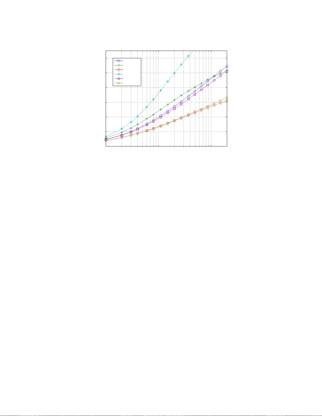
JMLR: W orkshop and Conference Pro ceedings v ol (2011) 1 – 18 25th Annu al Conference on Learning Theory The KL-UCB Algorithm for Bounded Sto chasti c Band its and Bey ond Aur´ elien Garivier and Olivier Capp ´ e garivier,cappe@telecom-p aristech.fr L TCI, CNRS & T ele c om Pari sT e ch, Paris, F r anc e Editor: Sha m Kak ade, Ulrike von Luxburg Abstract This paper presen ts a finite-time ana lysis o f the KL-UCB algor ithm, an online, horizo n- free index p olicy for sto ch astic bandit problems. W e prov e t w o distinct results: first, for arbitra r y b ounded r ew ards, the KL-UCB algor ithm s atisfies a uniformly b etter regret bo und than UCB and its v ariants; second, in the sp ecial ca se of Bernoulli rewards, it reaches the low er b ound of Lai and Robbins. F urthermore, we show that s imple adaptatio ns of the KL-UCB algo rithm ar e also optimal for sp ecific cla sses o f (p ossibly un b ounded) rewards, including those gene r ated from exp onential families of distributions. A la r ge-scale nu merical study co mparing KL-UCB w ith its main comp etitors (UCB, MOSS, UCB-T uned, UCB-V, DMED) shows that KL-UCB is remark ably efficie n t and stable, including for short time ho rizons. KL -UCB is a lso the o nly metho d that always p erforms b etter than the basic UCB p olicy . Our regre t b ounds rely on deviations r esults of indepe ndent interest which ar e stated and prov ed in the App e ndix. As a b y-pro duct, we also obtain a n improv ed regret bo und for the standard UCB alg orithm. Keyw ords: List o f keyw ords 1. In tro duction The m ulti-armed b andit prob lem is a simple, arc het ypal setting of reinf orcemen t learning, where an agen t facing a slot mac h ine with sev eral arms tries to maximize her profit b y a prop er c hoice of arm d ra ws. In the sto c hastic 1 bandit problem, the agen t sequentia lly c ho oses, f or t = 1 , 2 , . . . , n , an arm A t ∈ { 1 , . . . , K } , and r eceiv es a r ew ard X t suc h that, conditionally on the arm choic es A 1 , A 2 , . . . , the r ew ards are ind ep enden t and identi cally distributed, with exp ectatio n µ A 1 , µ A 2 , . . . . Her p olicy is the (p ossibly randomized) decision rule that, to ev ery past observ ations ( A 1 , X 1 , . . . , A t − 1 , X t − 1 ), asso ciates her n ext c hoice A t . The b est c hoice is an y arm a ∗ with maximal exp ected reward µ a ∗ . The p er f ormance of her p olicy can b e measured b y th e r e gr et R n , defined as the difference b etw een the rew ards she accum ulates u p to th e horizon t = n , and the rew ards that sh e would h a v e accumulat ed during the same p erio d, had sh e kn o wn from the b eginning whic h arm had the h ighest exp ected rew ard. The agent typical ly faces an “exploration versus exploitation dilemma” : at time t , she can tak e adv antag e of the in f ormation sh e h as gathered, by c ho osing the so-far b est p erforming arm , but she has to consider th e p ossibilit y that the other arm s are actually 1. An other in teresting setting is th e adversarial b an d it problem, where the rewards are not stochastic but chos en by an opp onen t - th is setting is not the sub ject of this pap er. c  2011 A. Garivier & O. Capp´ e. Garivier Capp ´ e under-rated an d she must p la y su fficien tly often all of them. Since the works of Gittins ( 1979 ) in th e 1970s, this problem raised m uc h in terest and sev eral v ariants, solutions and extensions ha v e b een pr op osed, s ee Ev en-Dar et al. ( 2002 ) and references therein. Tw o families of b andit s ettings can be distinguish ed: in the fir s t family , the d istribution of X t giv en A t = a is assu med to b elong to a f amily { p θ , θ ∈ Θ a } of probability distributions. In a particular p arametric framewo rk, Lai and Robbins ( 1985 ) prov ed a lo w er-b ound on the p erformance of any p olicy , and determined optimal policies. Th is fr amework w as ext ended to multi-paramete r mo dels b y Bu r netas and Katehakis ( 1997 ) w h o sho we d that th e n umb er of draws up to time n , N a ( n ), of an y sub -optimal arm a is lo w er-b ound ed b y N a ( n ) ≥  1 inf θ ∈ Θ a : E [ p θ ] >µ a ∗ K L ( p θ a , p θ ) + o (1)  log( n ) , (1) where K L denotes the Ku llbac k-Leibler div ergence and E ( p θ ) is the exp ectation und er p θ ; hence, the regret is lo w er-b ound ed as follo ws: lim in f n →∞ E [ R n ] log( n ) ≥ X a : µ a <µ a ∗ µ a ∗ − µ a inf θ ∈ Θ a : E [ p θ ] >µ a ∗ K L ( p θ a , p θ ) . (2) Recen tly , Honda and T ak emura ( 2010 ) prop osed an algorithm called Deterministic Mini- mum Empiric al D iver genc e (DMED) whic h they pro ve d to b e firs t order optimal. This algorithm, whic h main tains a list of arms that are cl ose enough to the b est one (and whic h th us m ust b e p la y ed), is inspired by large deviations ideas and r elies on the a v ailabilit y of the rate function asso ciated to the rewa rd distrib ution. In the second family of b andit pr oblems, the rewa rds are only assumed to b e b oun ded (sa y , b etw een 0 and 1), and p olic ies r ely directly on the estimates of the exp ected r ew ards for eac h arm. Th e KL -UCB algorithm considered in this p ap er is primarily m ean t to address this second, non-parametric, se tting. W e will nonetheless sho w that KL-UCB also matc hes the lo w er b oun d of Burnetas and Katehakis ( 1997 ) in the b inary case and that it can b e extended to a larger class of parametric band it problems. Among all th e bandit p oli cies that h av e b een p rop osed, a particular family h as raised a strong interest, after Gittins ( 1979 ) pro v ed th at (in the Ba y esian setting he considered ) optimal p olic ies could b e chosen in the follo w ing very s p ecia l form: compute for eac h arm a dynamic al lo c ation index (whic h only dep ends on the dra ws of this arm), and simp ly c ho ose an arm with maximal index. These p olicies not only compute an estimate of the exp ected rewa rds, bu t r ather an upp er- c onfidenc e b ound (UCB), and the agen t’s c hoice is an arm with highest UCB. T h is app roac h is sometimes called “optimistic”, as the agen t acts as if, at eac h instan t, th e exp ected rew ards were equal to the highest p ossible v alues that are compatible with her past observ ations. Auer et al. ( 2002 ), follo win g Agra w al ( 1995 ), prop osed and analyzed t w o v ariants, UCB1 (u sually called sim p ly UCB in latter works) and UCB2, f or whic h they p ro vided regret b oun ds. UCB is an on lin e, horizon-free pro cedure for whic h ( Auer et al. , 2002 ) pr o v es that there exists a constan t C suc h that E [ R n ] ≤ X a : µ a <µ a ∗ 8 log ( n ) ( µ a ∗ − µ a ) + C . (3) 2 KL-UCB: bounded bandits, and beyond The UCB2 v arian t relies on a paramete r α that n eeds to b e t uned , d ep ending in particular on the horizon, and satisfies the tight er regret b ound E [ R n ] ≤ X a : µ a <µ a ∗ (1 + ǫ ( α )) log( n ) 2 ( µ a ∗ − µ a ) + C ( α ) , where ǫ ( α ) > 0 is a constan t that can get arb itrary small w hen α is small, at the ex- p ense of an increased v alue of the constant C ( α ). The constant 1 / 2 in fr on t of the factor log( n ) / ( µ a ∗ − µ a ) cannot b e im p ro v ed. W e sho w in Prop osition 4 , as a b y-pro du ct of our analysis, that a correctly tuned UCB algorithm satisfies a similar b ound. Ho w ev er, Auer et al. ( 2002 ) found in n umerical exp eriment s that UCB and UCB2 we re outp erformed b y a thir d heuristic v arian t called UCB-T uned, w hic h includes estimates of the v ariance, but no th eoretic al guarant ee w as giv en. In a latter work, Audib ert et al. ( 2009 ) prop osed a related p olicy , called UCB-V, whic h uses an empirical v ersion of the Bernstein b ound to obtain refi ned upp er confidence b ounds. Recen tly , Audib ert and Bub ec k ( 2 010 ) in tro d uced an impro v ed UCB algorithm, termed MOSS, which ac hiev es th e distribu tion-free optimal rate. In this contribution, we fir st consider the stochastic , n on-parametric, b oun ded ban- dit p r oblem. W e consider an online in d ex p olicy , called KL-UCB (for Kullbac k-Leibler UCB), that r equires no p roblem- or horizon-dep endent tuning. This algorithm was r ecen tly adv o cated by Filippi ( 2010 ), together with a s im ilar pr ocedu re for Mark o v Decision Pro- cesses ( Filippi et al. , 2010 ), and w e learnt since our in itial submission that an analysis of the Bernoulli case can also b e found in Maillard et al. ( 2011 ), together with other results. W e pro v e in Theorem 1 b elo w that the regret of KL-UCB satisfies lim s u p n →∞ E [ R n ] log( n ) ≤ X a : µ a <µ a ∗ µ a ∗ − µ a d ( µ a , µ a ∗ ) , where d ( p, q ) = p log( p/q ) + (1 − p ) log((1 − p/ (1 − q )) d enotes the Kullback-Le ibler div er- gence b et ween Bernoulli distribu tions of parameters p and q , resp ectiv ely . This comes as a consequence of Theorem 2 , a non-asymptotic upp er -b ound on the num b er of draws of a sub-optimal arm a : for all ǫ > 0 th ere exist C 1 , C 2 ( ǫ ) and β ( ǫ ) su c h that E [ N n ( a )] ≤ log( n ) d ( µ a , µ a ∗ ) (1 + ǫ ) + C 1 log(log ( n )) + C 2 ( ǫ ) n β ( ǫ ) . W e in sist on the fact that, desp ite the presence of diverge nce d , this b oun d is not sp ecific to the Bernoulli case and app lies to all reward distr ib utions b ounded in [0 , 1] (and th us, b y rescaling, to all b ound ed rew ard distribu tions). By Pinsker’s in equalit y , d ( µ a , µ a ∗ ) > 2( µ a − µ a ∗ ) 2 , and thus KL-UCB has strictly b etter theoretical guarante es than UCB, while it has the same range of application. T he improv ement app ears to b e significant in sim ulations. Moreo v er, KL-UCB is the fir st index p olicy that reac hes the low er-b ound of Lai and Robbins ( 1985 ) for binary rewards; it do es also ac hiev e lo w er regret than UCB-V in that case. Hence, KL-UCB is b oth a general-purp ose pro cedure for b ou n ded bandits, and an optimal solution for the binary case. F ur thermore, it is easy to adapt KL-UCB to p articular (p ossibly n on-b ounded) bandit settings, w hen the distribution of rew ard is kno wn to b elo ng to some family of p robabilit y 3 Garivier Capp ´ e la ws. By simp ly changing the d efinition of the divergence d , optimal algorithms may b e built in a great v ariet y of situations. The pro ofs w e giv e for th ese results a re short and elementa ry . They r ely on devia- tion results for b ounded v ariables that are of indep en den t interest : Lemma 9 sho ws that Bernoulli v ariable are, in a sense, the “least concen trated” b oun d ed v ariables with a giv en exp ectation (as is well-kno w n for v ariance) , and Th eorem 10 sho ws an efficien t wa y t o bu ild confidence i nte rv als for sums of b ounded v ariables with an unkno wn num b er of summands . In practice, n umerical exp erimen ts confir m the significant adv an tage of KL -UCB ov er existing pro cedures; not only do es this m etho d outp erform UCB, MOS S, UCB-V and ev en UCB-tuned in v arious scenarios, but it also compares w ell to DMED in the Be rnoulli case, esp ecially for small or mo derate horizons. The pap er is organized as follo ws: in S ectio n 2 , we int ro duce some nota tion a nd p r esen t the KL-UCB algorithm. Section 3 conta ins t he main results of the pap er, n amely the regret b ound for KL-UCB and the optimalit y in the Bernoulli case. In Section 4 , w e show ho w to adapt the KL-UCB algorithm to address general families of r eward distr ibutions, and w e p ro vide finite-time regret b ounds sho wing asymp totic optimalit y . Section 5 r ep orts the results of extensive numerical exp eriments, showing the practical sup eriorit y of KL-UCB. Section 6 is dev oted to an elemen tary pro of of the main theorem. Finally , the App endix gathers some deviatio n results that are useful in th e pro ofs of our regret b ound s, but which are also of indep end en t i nte rest. 2. The KL-UCB Algorithm W e consider the follo wing bandit p roblem: the set of actions is { 1 , . . . , K } , w here K de- notes a finite intege r. F or eac h a ∈ { 1 , . . . , K } , the rewa rds ( X a,t ) t ≥ 1 are ind ep enden t and b ounded 2 in Θ = [0 , 1] with common exp ectation µ a . The sequences ( X a, · ) a are ind ep en- den t. At eac h time step t = 1 , 2 , . . . , the ag en t c ho oses an action A t according to his past observ ations (p ossibly usin g some indep endent rand omizat ion) and gets th e rew ard X t = X A t ,N A t ( t ) , where N a ( t ) = P t s =1 1 { A s = a } denotes the n umb er of times action a w as c hosen up to time t . The sum of rew ards she h as obtained when c ho osing action a is denoted b y S a ( t ) = P s ≤ t 1 { A s = a } X s = P N a ( t ) s =1 X a,s . F or ( p, q ) ∈ Θ 2 denote the Bernoulli Kullbac k-Leibler diverge nce b y d ( p, q ) = p log p q + (1 − p ) log 1 − p 1 − q , with, b y conv entio n, 0 log 0 = 0 log 0 / 0 = 0 and x log x/ 0 = + ∞ for x > 0. Algorithm 1 pro vides th e pseud o-code for KL -UCB. On line 6, c is a parameter th at, in the regret b ound stated b elo w in Th eorem 1 is chosen equal to 3; in practice, how ev er, we recommend to tak e c = 0 for optimal p erformance. F or eac h arm a the upp er-confidence b ound max  q ∈ Θ : N [ a ] d  S [ a ] N [ a ] , q  ≤ log ( t ) + c log(log ( t ))  can b e efficiently co mpu ted u sing Newton iterations, as for an y p ∈ [0 , 1] the function q 7→ d ( p, q ) is strictly conv ex and increasing on the interv al [ p, 1]. I n case of ties b et w een 2. if the rew ards are b ounded in another interv al [ a , b ], they should first b e rescaled to [0 , 1]. 4 KL-UCB: bounded bandits, and beyond Algorithm 1 KL-UCB Require: n (h orizon), K (num b er of arm s), REW ARD (reward function, b oun ded in [0 , 1]) 1: for t = 1 to K do 2: N [ t ] ← 1 3: S [ t ] ← REW ARD(arm = t ) 4: end for 5: for t = K + 1 to n do 6: a ← arg max 1 ≤ a ≤ K max n q ∈ Θ : N [ a ] d  S [ a ] N [ a ] , q  ≤ log ( t ) + c log(log ( t )) o 7: r ← REW ARD(arm = a ) 8: N [ a ] ← N [ a ] + 1 9: S [ a ] ← S [ a ] + r 10: end for sev erals arms, an y maximizer can b e chosen (for instance, at random). The KL-UCB elab orates on ideas suggested in Sections 3 and 4 of Lai and Robbins ( 1985 ). 3. Regret b ounds and optimalit y W e first s tate the main result of th is pap er. It is a d ir ect consequence of the non-asymp totic b ound in Theorem 2 stated b elo w. Theorem 1 Consider a b andit pr oblem with K arms and indep endent r ewar ds b ounde d in [0 , 1] , and deno te by a ∗ an optimal arm. Cho osing c = 3 , the r e g r et of the KL-UCB algorithm satisfies: lim s u p n →∞ E [ R n ] log( n ) ≤ X a : µ a <µ a ∗ µ a ∗ − µ a d ( µ a , µ a ∗ ) . Theorem 2 Consider a b andit pr oblem with K arms and indep endent r ewar ds b ounde d in [0 , 1] . L et ǫ > 0 , and take c = 3 in Algorithm 1 . L et a ∗ denote an arm with maximal exp e cte d r ewar d µ a ∗ , and let a b e an arm such that µ a < µ a ∗ . F or any p ositive inte ger n , the numb er of times algorithm KL-UCB cho oses arm a is upp er-b ounde d by E [ N n ( a )] ≤ log( n ) d ( µ a , µ a ∗ ) (1 + ǫ ) + C 1 log(log ( n )) + C 2 ( ǫ ) n β ( ǫ ) , wher e C 1 denotes a p ositive c onstant and wher e C 2 ( ǫ ) and β ( ǫ ) denote p ositive functions of ǫ . H enc e, lim s u p n →∞ E [ N n ( a )] log( n ) ≤ 1 d ( µ a , µ a ∗ ) . Corollary 3 If the r ewar d distributions ar e Bernoul li, the KL-UCB algorithm is asymp- totic al ly optimal, in the sense that the r e gr et of KL-UCB matches the lower-b ound pr ove d by L ai and R obbins ( 1985 ) and g ener alize d by Burnetas and Katehakis ( 1997 ): N n ( a ) ≥  1 d ( µ a , µ a ∗ ) + o (1)  log( n ) 5 Garivier Capp ´ e with a pr ob ability tending to 1 . The KL -UCB algorithm th us app ears to b e (asymptoticall y) optimal for Bernoulli re- w ards. Ho w ev er, Lemma 9 sho ws that the Chernoff b ou n ds obtained for Bernoulli v ariables actually apply to an y v ariable with range [0 , 1]. T h is is why K L-UCB is not only efficien t in the binary case, but also for general b oun d ed rew ards. As a b y-pro duct, we obtain an impr o v ed u pp er-b ound for the regret of the UCB algo- rithm: Prop osition 4 Consider the UCB algorithm tune d as fol lows: at step t > K , the arm tha t maximizes the upp er- b ound S [ a ] / N [ a ] + p (log( t ) + c log log( t )) / (2 N [ a ]) is chosen. Then, for the choic e c = 3 , the numb er of dr aws of a sub -optimal arm a is upp er-b ounde d as: E [ N n ( a )] ≤ log( n ) 2( µ a − µ a ∗ ) 2 (1 + ǫ ) + C 1 log(log ( n )) + C 2 ( ǫ ) n β ( ǫ ) . (4) This b ound is “optimal”, in the sense that th e constan t 1 / 2 in the loga rithmic term cannot b e imp ro v ed. The p ro of of this p rop osition j u st mimics that of S ection 6 (whic h concerns KL-UCB), u s ing the quadr atic div ergence d ( p, q ) := 2( p − q ) 2 instead of the Kullback-Le ibler div ergence; it is thus omitted. In cont rast, Pinske r’s inequalit y d ( µ a , µ a ∗ ) ≥ 2( µ a − µ a ∗ ) 2 sho ws that KL-UCB dominates UCB, and we will see in the simulat ion study that th e difference is significan t, even for smaller v alues of the h orizon. Remark 5 At line 6 , Algorithm 1 c omputes for e ach arm a ∈ { 1 , . . . , K } the upp er- c onfidenc e b ound max  q ∈ Θ : N [ a ] d  S [ a ] N [ a ] , q  ≤ log ( t ) + c log(log ( t ))  . The level of this c onfidenc e b ound is p ar ameterize d by the explor ation function log ( t ) + c log (log ( t )) , an d the r esults of The or ems 1 and 2 ar e true a s so on as c ≥ 3 . However, similar r esu lts c an b e pr ove d with an explor ation function e qual to (1 + ǫ ) log( t ) (inste ad of log( t ) + c log(log ( t )) ) for every ǫ > 0 ; this is no surprise, as (1 + ǫ ) log ( t ) ≥ log ( t ) + c log (log ( t )) when t is lar ge enough. But “lar ge enough”, in that c ase, c an b e quite lar ge : for ǫ = 0 . 1 , this holds true only for t > 2 . 10 51 . This is why, in pr actic e (a nd for the simulat ions pr esente d in Se ction 5 ), we r ather sugge st to cho ose c = 0 . 4. KL-UCB for parametric families of reward distributions The KL-UCB algorithm mak es no assum p tion on th e distribu tion of the rew ards, except that they are b ou n ded. Actually , the defin ition of the div ergence function d in KL-UCB is dictated by the rate fu nction of the Large Deviations Principle satisfied b y Bernoulli random v ariables: th e p ro of of Theorem 10 relies on the control of the F enc hel-Lege ndr e transform of the Bernoulli distribution. Thanks to L emma 9 , th is c hoice also mak es sense for all b ounded v ariables. But the metho d presente d here is n ot limited to th e Bernoulli case: K L-UCB can ve ry easily b e adapted to other settings by c ho osing an ap p ropriate dive rgence f unction d . As an 6 KL-UCB: bounded bandits, and beyond illustration, w e will a ssume in this sec tion that, for eac h arm a , the distribution of rewards b elongs to a c anonic al exp onentia l family , i.e., that its densit y with resp ect to some referen ce measure can b e written as p θ a ( x ) for some real parameter θ a , with p θ ( x ) = exp ( xθ − b ( θ ) + c ( x )) , (5) where θ is a real parameter, c is a real function and the log -partition f unction b ( · ) is assum ed to b e twice differen tiable. This family conta ins f or instance the Exp onential, Poi sson, Gaussian (with fixed v ariance), Ga mma (with fixed shap e p arameter) distributions (as well as, of course, the Bern ou lli distribution). F or a random v ariable X with density defined in ( 5 ), it is easily c hec k ed that µ ( θ ) , E θ [ X ] = ˙ b ( θ ); moreo v er, as ¨ b ( θ ) = V ar ( X ) > 0, the function θ 7→ µ ( θ ) is one-to-one. Theorem 11 (in the App endix) sta tes that the prob ab ility of under-estimating the p erformance of th e b est arm can b e upp er-b ou n ded just as in the Bernoulli case b y rep lacing the div ergence d ( · , · ) in lin e 6 of the KL-UCB algorithm by d ( x, µ ( θ )) = sup λ { λx − log E θ [exp( λX )] } . F or example, in the case of exp onent ial rewards, one should choose d ( x, y ) = x/y − 1 − log( x/y ). Or, f or Poisson rewa rds , the righ t choic e is d ( x, y ) = y − x + x log( x/y ). Then, all the results stated ab ov e app ly (as the pro ofs do n ot in v olv e the p articular form of the function d ), and in particular : lim s u p n →∞ E [ R n ] log( n ) ≤ X a : µ a <µ a ∗ µ a ∗ − µ a d ( µ a , µ a ∗ ) . In order to p ro v e that, for those f amilies of rew ards, th is v ersion of the KL-UCB al- gorithm matc hes the b ound of Lai and Robbins ( 1985 ) , it r emains only to show that d ( x, y ) = K L ( p µ − 1 ( x ) , p µ − 1 ( y ) ). This is the ob ject of Lemma 6 . Generalizatio ns to other families of rewa rd d istributions (p ossibly differen t fr om arm to arm) are conceiv able, b ut require more tec hnical, t op ological discussions , as in Bur netas and Katehakis ( 1997 ) and Honda and T ak emura ( 2010 ). T o conclude, observe that it is n ot required to work with th e d iv ergence function d corre- sp onding exactly to th e family of rew ard distribu tions: u sing an up p er-b ound in stead often leads to more simple and v ersatile p olicies at th e pr ice of only a sligh t loss in p erformance. This is illustrated in th e third scenario of the simulatio n study pr esen ted in Section 5 , bu t also b y Theorems 1 and 2 for b ounded v ariables. Lemma 6 L et ( β , θ ) b e two r e al numb ers, let p β and p θ b e two pr ob ability densities of the c anonic al exp onential f amily define d in ( 5 ) , and let X have density p θ . Then Kul lb ack- L eibler diver genc e K L ( p β , p θ ) is e qual to d ( µ ( β ) , µ ( θ )) . Mor e pr e cisely, K L ( p β , p θ ) = d ( µ ( β ) , µ ( θ )) = µ ( β ) ( β − θ ) − b ( β ) + b ( θ ) . Pro of First, it holds that K L ( p β , p θ ) = Z exp ( xβ − b ( β ) + c ( x )) { x ( β − θ ) − b ( β ) + b ( θ ) } dx = µ ( β ) ( β − θ ) − b ( β ) + b ( θ ) . 7 Garivier Capp ´ e Then, observe that E [exp( λX )] = R exp ( x ( β + λ ) − b ( β ) + c ( x )) dx = exp( b ( β + λ ) − b ( β )) . Th us, for ev ery x the maxim um of the (smo oth, conca v e) fu n ction λ 7→ λx − log E [exp( λX )] = λx − b ( θ + λ ) + b ( θ ) is reac hed for λ = λ ∗ suc h that x = ˙ b ( θ + λ ∗ ) = µ ( θ + λ ∗ ). Th us, if x = µ ( β ), the fact that µ is one-to-o ne implies that θ + λ ∗ = β and thus that: d ( µ ( β ) , µ ( θ )) = ( β − θ ) µ ( β ) − b ( β ) + b ( θ ) . 5. Numerical exp erimen ts and comparisons of t he p olicies Sim ulations studies require particular atten tion in the case of bandit algorithms. As p ointed out by Audib ert et al . ( 2009 ), for a fi x ed horizon n the distribution of the regret is ve ry p o orly concen trated aroun d its exp ectation. This can b e e xplained as follo ws: most of the time, the estimates of al l arms remain correctly ordered for almost all instan ts t = 1 , . . . , n and the r egret is of order log ( n ). But sometimes, at the b eginnin g, the b est arm is und er- estimated wh ile one of th e sub-optimal arms is o v er-estimate d, so that the agen t k eeps pla ying the latter; and as she neglects the b est arm, s he has h ardly an o ccasion to realize h er mistak e, and the error p erp etuates for a ve ry long time. Th is happ ens with a small, bu t not negligible probabilit y , b ecause th e regret is very imp ortan t (of order n ) on these occasions. Bandit algorithms are t ypically d esigned to con trol th e probabilit y of suc h adve rse ev en ts but usually at a rate which only deca ys sligh tly faster than 1 /n , which results in v ery sk ew ed regret distributions with slowly v anishing upp er tails. 10 2 10 3 10 4 0 50 100 150 200 250 300 350 400 450 500 n (log scale) N 2 (n) UCB MOSS UCB−Tuned UCB−V DMED KL−UCB bound 0 500 1000 1500 2000 2500 3000 3500 4000 UCB MOSS UCB−Tuned UCB−V DMED KL−UCB N 2 (n) Figure 1: Performance of the v arious algorithms in the simple t w o arms, scenario. Left, mean n umber of draws of the su b optimal arm as a fu nction of time; right, b o x- plots sho wing the d istr ibutions of the n umber of dra ws of the sub optimal arm at time n = 5 , 000 . Results based on 50 , 000 ind ep enden t runs. 8 KL-UCB: bounded bandits, and beyond 5.1. Scenario 1: tw o arms W e first consider the basic t w o arm scenario with Bernoulli rewa rds of exp ectations µ 1 = 0 . 9 and µ 2 = 0 . 8, resp ectiv ely . The left panel of Figure 1 sho ws the a v erage num b er of dr a ws of the su b optimal arm a s a function of time (on a lo garithmic scale) for KL-UCB c ompared to five b enchmark alg orithms (UCB, MOSS, UCB-T uned, UCB-V and DMED). T he righ t panel of Figure 1 sho ws the empirical distribu tions of sub optimal draws, represent ed as b o x-and-whiskers plots, at a particular time ( t = 5 , 000) for all six algorithms. Th ese plot are obtained from N = 50 , 000 indep en d en t ru ns of the algorithms and the right panel of Figure 1 clearly highlight the tail effect m en tioned ab o v e. On this v ery simp le example, w e observed that results obtained from N = 1 , 000 or less simulat ions w ere not r eliable, t ypically resulting in a significant o v er-estimatio n 3 of the p erform an ce of “risky” algorithms, in particular of UCB-T uned . More generally , results obtained in configurations where N is m uc h smaller than n are like ly to b e unreliable. F or t his reason, we limit our in v estigations to a final instan t of n = 20 , 000. Note ho w ev er that the av erag e num b er of sub optimal dra ws of most algorithms at n = 20 , 000 is on ly of the order of 300, sho wing th at there is no p oin t in considering larger horizons for su c h a simple problem. MOSS, UCB-T uned and UCB-V are r u n exac tly as describ ed by Audib ert and Bub ec k ( 2010 ), Auer et al. ( 2002 ) and Audib ert et al. ( 2009 ), resp ectiv ely . F or UCB, we u se an upp er confidence b ound S [ a ] / N [ a ] + p log( t ) / (2 N [ a ]) , as in Pr op osition 4 , again with c = 0. Note that in our tw o arm scenario, { 2( µ 1 − µ 2 ) 2 } − 1 = 50 while d − 1 ( µ 2 , µ 1 ) = 2 2 . 5. Hence, the p erformance of DMED and KL-UCB should b e ab out t w o times b ette r than that of UCB. Th e left p an el of Figure 1 do es sho w th e exp ected b eha vior but with a d ifference of lesser magnitud e. Indeed, one can o bserve that the boun d d − 1 ( µ 2 , µ 1 ) log ( n ) (shown in dashed lin e) is quite p essimistic for the v alues of the horizon n considered here as th e actual p er f ormance of K L-UCB is significan tly b elo w the b ound. F or DMED, w e follo w Honda and T ak emura ( 2010 ) but using N [ a ] d  S [ a ] N [ a ] , m ax b S [ b ] N [ b ]  < log t (6) as the criterion to d ecide w hether arm a should b e included in th e list of arms to be play ed. This criterion is clearly relat ed to the d ecisio n rule us ed b y KL-UCB when c = 0 (see line 6 of Algorithm 1 ) except for the fact that in KL -UCB the estimate S [ a ] / N [ a ] is not compared to that of the curren t b est arm max b S [ b ] / N [ b ] but to the corresp onding upp er confidence b ound. As a consequence, an y arm that is not included in the list of arms to b e pla y ed b y DMED would not b e play ed by KL-UCB either (assuming that b oth algorithms sh are a common history). As one can observ e on the left panel of Figure 1 , this results in a degraded p erformance for DMED. W e also observed this effect on UCB, for instance, and it seems that index algorithms are generally p r eferable to their “arm eliminatio n” v arian t. The original prop osal of Honda and T ak emura ( 2010 ) consists in using in the exp loration function a f actor log ( t/ N [ a ]) instead of log( t ), as in th e MOS S algorithm. As will b e seen b elo w on Figure 2 , th is v arian t (wh ic h w e refer to as DM ED+) indeed outp erform s DMED. But our pr evious conjecture app ears to h old also in th is case a s th e heuristic v arian t of KL- 3. In cid entally , Theorem 10 could b e used to construct sharp confidence b ounds for the regret. 9 Garivier Capp ´ e UCB (termed K L-UCB+) in which log( t ) in line 6 of Algorithm 1 is r ep lace d by log ( t/ N [ a ]) remains preferable to DMED+. As final comments on Figure 1 , first note that UCB-T un ed p erforms as exp ected — though sligh tly w orse than KL-UCB— but is a v ery risky algorithm: the righ t p anel of Figure 1 casts some dou b ts on the fact that the tails of N a ( n ) are indeed con trolled u ni- formly in n for UCB-T u ned. Second, the p erf ormance of UCB-V is somewhat disapp ointing. Indeed, the upp er-confidence b ounds o f UCB-V differ from th ose of UCB-T uned simply b y the n on-asymptotic c orrection term 3 log( t ) / N [ a ] required b y Bennett’s an d Bernstein’s in- equalities ( Au d ib ert et al. , 2009 ). This correction term app ears to hav e a significan t im p act on mo derate time h orizons: for a sub -optimal arm a , the num b er of draws N [ a ] do es not gro w faster than the log ( t ) exploration function, and log ( t ) / N [ a ] do es not v anish . 0 100 200 300 400 500 10 2 10 3 10 4 R n UCB 0 100 200 300 400 500 10 2 10 3 10 4 MOSS 0 100 200 300 400 500 10 2 10 3 10 4 UCB−V 0 100 200 300 400 500 10 2 10 3 10 4 R n UCB−Tuned 0 100 200 300 400 500 10 2 10 3 10 4 DMED 0 100 200 300 400 500 10 2 10 3 10 4 KL−UCB 0 100 200 300 400 500 10 2 10 3 10 4 n (log scale) R n CP−UCB 0 100 200 300 400 500 10 2 10 3 10 4 n (log scale) DMED+ 0 100 200 300 400 500 10 2 10 3 10 4 n (log scale) KL−UCB+ Figure 2: Regret of the v arious algorithms as a fu nction of time (on a log scale) in the ten arm scenario. On eac h graph, th e red d ash ed line sh o ws the lo wer b ound, the solid b old curv e corresp onds to the mean r egret while the dark and ligh t sh aded regions show r esp ectiv ely the cen tral 99% region and the u pp er 0.05% quanti le, resp ectiv ely . 10 KL-UCB: bounded bandits, and beyond 5.2. Scenario 2: lo w rewards In Figure 2 we consid er a significantl y m ore difficult scenario, again w ith Bernoulli rewards, inspired b y a situati on (frequent in applications lik e mark eting or In ternet adv ertising) where the mean reward of eac h arm is very lo w. In this scenario, there are ten arms: the optimal arm has exp ected reward 0.1, and the nine sub optimal arms consist of three differen t groups of three (sto c hastically) iden tical arm s eac h with exp ected rewards 0.05, 0.02 and 0.01, r esp ectiv ely . W e aga in used N = 50 , 000 sim ulations to obtain the regret plots of Figure 2 . These plots sh ow, for eac h alg orithm, the a v erage cum ulated regret together w ith quan tiles of the cum ulated regret distribution as a fun ction of time (again on a logarithmic scale). In this scenario, th e difference is more pronounced b etw een UCB and K L-UCB. Th e p erformance gain of UCB-T uned is also m uch less significan t. KL-UCB and DMED reac h a p erformance that is on par with the low er b ound of Burnetas and Katehakis ( 1997 ) in ( 2 ), although the p erformance of K L-UCB is here again significan tly b etter. Using KL-UCB+ and DMED+ r esults in significant mean impr ov emen ts, although th ere are hint s th at those algorithms migh t indeed b e to o risky w ith o ccasional very large deviations fr om th e mean regret curv e. The final algorithm included in this roundu p, called CP-UCB, is in some sense a furth er adaptation of KL -UCB to the sp eci fic case of Bernoulli rewards. F or n ∈ N and p ∈ [0 , 1], denote b y P n,p the b in omial distrib ution with parameters n and p . F or a random v ariable X with distribution P n,p , th e Clopp er-Pe arson (see Clopp er and Pearson ( 1934 )) or “exact” upp er-confid ence b ound of risk α ∈ ]0 , 1[ for p is u C P ( X, n, α ) = max { q ∈ [0 , 1] : P n,q ([0 , X ]) ≥ α } . It is easily verified th at P n,p  µ ≤ u C P ( X )  ≥ 1 − α , and that u C P ( X ) is the small est quan tit y s atisfying this prop erty: u C P ( X ) ≤ ˜ u ( X ) for an y other up p er-confidence b oun d ˜ u ( X ) of risk at most α . The Clopp er-P earson Upp er-Confid en ce Bound algorithm (CP-UCB) differs f rom KL- UCB only in the wa y the up p er-confidence b ound on th e p erformance of eac h arm is com- puted, replacing line 6 of Algorithm 1 b y a ← arg max 1 ≤ a ≤ K u C P  S [ a ] , N [ a ] , 1 t log( t ) c  . As the Clopp er-Wilso n confidence inte rv als are alw a ys sh arp er th an the Kullback-Le ibler in terv als, one can v ery easily adapt the pro of of Section 6 to sho w that the regret b ounds pro v ed for the KL-UCB algorithm also hold for CP-UCB in the case of Bernoulli r ew ards. Ho w ev er, the impr o v emen t o v er K L-UCB is v ery limited (often, the t w o algorithms actually tak e exactly the same decisions). In terms of resu lts, one can observe on Figure 2 that C P - UCB only ac hiev es a p erformance that is marginally b etter than that of KL-UCB. Besides, there is no guaran tee that the CP-UCB algorithm is also efficien t on arbitrary b ounded distributions. 5.3. Scenario 3: b ounded exp onential rewards In the third examp le, there are 5 arms: the r ew ards are exp onent ial v ariables, with param- eters 1 / 5, 1 / 4, 1 / 3, 1 / 2 and 1 resp ect iv ely , truncated at x max = 10 (th us, they are b oun ded 11 Garivier Capp ´ e 10 2 10 3 10 4 0 200 400 600 800 1000 1200 n (log scale) R n UCB MOSS UCB−Tuned UCB−V KL−UCB KL−UCB−exp Figure 3: Regret of the v arious algorithms as a fun ction of time in the b ounded exp onential scenario. in [0 , 10]). The interest of th is scenario is t w ofold: first, it s h o ws the p erformance of KL- UCB for non-binary , non-discrete, n on [0 , 1]-v alued rew ards. Second, it illustrates that, as explained in Section 4 , sp ecific v arian ts of the KL-UCB algorithm can r eac h an even b ett er p erformance. In this scenario, UCB and MOSS, but also K L -UCB are clearly sub-optimal. UCB- T uned and UCB-V, by taking in to accoun t the v ariance of the rew ard distr ib utions (m uc h smaller than the v ariance of a { 0 , 10 } -v alued d istribution with the same exp ect ation), w ere exp ected to p erform significan tly b etter. F or the reasons men tionned ab o ve this is not the case f or UCB-V on a time horizo n n = 20 , 000. Y et, UCB-T uned is s p ecta cularly more efficient , and is only caugh t up by KL-UCB-exp, the v arian t of KL-UCB designed for exp onen tial r ewards. Actually , the KL-UCB-exp algo rithm ig nores the fact that the rew ards are truncated, and us es the diverge nce d ( x, y ) = x/y − 1 − log ( x/y ) p rescrib ed for gen uine exp onen tial d istributions. One can easily sho w that th is c hoice leads to sligh tly to o large upp er confid en ce b oun ds. Y et, the p erforman ce is still excellen t, stable, and the algorithm is particularly simple. 6. Pro of of Theorem 2 Consider a p ositiv e inte ger n , a small ǫ > 0, an optimal arm a ∗ and a sub-optimal arm a suc h th at µ a < µ a ∗ . Without loss of generalit y , w e will assume that a ∗ = 1. F or an y arm b , the past a v erage p erform an ce of arm b is d enoted by ˆ µ b ( t ) = S b ( t ) / N b ( t ); b y con v enience, f or ev ery p ositiv e inte ger s w e will also den ote ˆ µ b,s = ( X b, 1 + · · · + X b,s ) /s , so that ˆ µ t ( b ) = ˆ µ b,N b ( t ) . KL-UCB relies on the follo wing u pp er-confidence b ound for µ b : u b ( t ) = max { q > ˆ µ b ( t ) : N b ( t ) d ( ˆ µ b ( t ) , q ) ≤ log ( t ) + 3 log(log( t )) } . 12 KL-UCB: bounded bandits, and beyond F or x, y ∈ [0 , 1], define d + ( x, y ) = d ( x, y ) 1 x u 1 ( t ) } # + E " n X t =1 1 { A t = a, µ 1 ≤ u 1 ( t ) } # ≤ n X t =1 P ( µ 1 > u 1 ( t )) + E " n X s =1 1 { sd + ( ˆ µ a,s , µ 1 ) < log ( n ) + 3 log(log( n )) } # , where the last inequalit y is a consequence of L emm a 7 . The fi r st su mmand is upp er-b ounded as follo ws: b y Th eorem 10 (p r o v ed in the App end ix), P ( µ 1 > u 1 ( t )) ≤ e ⌈ log( t ) (log( t ) + 3 log (log ( t ))) ⌉ exp( − log ( t ) − 3 log (log ( t ))) = e  log( t ) 2 + 3 log( t ) log (log( t ))  t log( t ) 3 . Hence, n X t =1 P ( µ 1 > u 1 ( t )) ≤ n X t =1 e  log( t ) 2 + 3 log( t ) log (log( t ))  t log( t ) 3 ≤ C ′ 1 log(log ( n )) for s ome p ositive constan t C ′ 1 ( C ′ 1 ≤ 7 is su fficien t). F or the second su mmand, let K n =  1 + ǫ d + ( µ a , µ 1 )  log( n ) + 3 log (log( n ))   . Then: n X s =1 P  sd + ( ˆ µ a,s , µ 1 ) < log ( n ) + 3 log (log( n ))  ≤ K n + ∞ X s = K n +1 P  sd + ( ˆ µ a,s , µ 1 ) < log ( n ) + 3 log (log( n ))  ≤ K n + ∞ X s = K n +1 P  K n d + ( ˆ µ a,s , µ 1 ) < log ( n ) + 3 log(log ( n ))  = K n + ∞ X s = K n +1 P  d + ( ˆ µ a,s , µ 1 ) < d ( µ a , µ 1 ) 1 + ǫ  ≤ 1 + ǫ d + ( µ a , µ 1 )  log( n ) + 3 log (log( n ))  + C 2 ( ǫ ) n β ( ǫ ) according to L emm a 8 . T his will conclude the pro of, provi ded that we prov e the follo wing t w o lemmas. Lemma 7 n X t =1 1 { A t = a, µ 1 ≤ u 1 ( t ) } ≤ n X s =1 1 { sd + ( ˆ µ a,s , µ 1 ) < log ( n ) + 3 log (log( n )) } . 13 Garivier Capp ´ e Pro of Observ e that A t = a and µ 1 ≤ u 1 ( t ) together imp ly th at u a ( t ) ≥ u 1 ( t ) ≥ µ 1 , and hence that d + ( ˆ µ a ( t ) , µ 1 ) ≤ d ( ˆ µ a ( t ) , u a ( t )) = log( t ) + 3 log (log( t )) N a ( t ) . Th us, n X t =1 1 { A t = a, µ 1 ≤ u 1 ( t ) } ≤ n X t =1 1 { A t = a, N a ( t ) d + ( ˆ µ a ( t ) , µ 1 ) ≤ log ( t ) + 3 log (log ( t )) } = n X t =1 t X s =1 1 { N t ( a ) = s, A t = a, sd + ( ˆ µ a,s , µ 1 ) ≤ log ( t ) + 3 log(log ( t )) } ≤ n X t =1 t X s =1 1 { N t ( a ) = s, A t = a } 1 { sd + ( ˆ µ a,s , µ 1 ) ≤ log ( n ) + 3 log(log ( n )) } = n X s =1 1 { sd + ( ˆ µ a,s , µ 1 ) ≤ log ( n ) + 3 log (log( n )) } n X t = s 1 { N t ( a ) = s, A t = a } = n X s =1 1 { sd + ( ˆ µ a,s , µ 1 ) ≤ log ( n ) + 3 log (log( n )) } , as, for ev ery s ∈ { 1 , . . . , n } , P n t = s 1 { N t ( a ) = s, A t = a } ≤ 1. Lemma 8 F or e ach ǫ > 0 , ther e exist C 2 ( ǫ ) > 0 and β ( ǫ ) > 0 such that ∞ X s = K n +1 P  d + ( ˆ µ a,s , µ 1 ) < d ( µ a , µ 1 ) 1 + ǫ  ≤ C 2 ( ǫ ) n β ( ǫ ) . Pro of If d + ( ˆ µ a,s , µ 1 ) < d ( µ a , µ 1 ) / (1 + ǫ ) , then ˆ µ a,s > r ( ǫ ), wh ere r ( ǫ ) ∈ ] µ a , µ 1 [ is suc h that d ( r ( ǫ ) , µ 1 ) = d ( µ a , µ 1 ) / (1 + ǫ ). Hence, P  d + ( ˆ µ a,s , µ 1 ) < d ( µ a , µ 1 ) 1 + ǫ  ≤ P ( d ( ˆ µ a,s , µ a ) > d ( r ( ǫ ) , µ a ) , ˆ µ a,s > µ a ) ≤ P ( ˆ µ a,s > r ( ǫ )) ≤ exp( − sd ( r ( ǫ ) , µ a )) , and ∞ X s = K n +1 P  d + ( ˆ µ a,s , µ 1 ) < d ( µ a , µ 1 ) 1 + ǫ  ≤ exp( − d ( r ( ǫ ) , µ a ) K n ) 1 − exp( − d ( r ( ǫ ) , µ a )) ≤ C 2 ( ǫ ) n β ( ǫ ) , with C 2 ( ǫ ) = (1 − exp( − d ( r ( ǫ ) , µ a ))) − 1 and β ( ǫ ) = (1 + ǫ ) d ( r ( ǫ ) , µ a ) /d ( µ a , µ 1 ). Easy com- putations show that r ( ǫ ) = µ a + O ( ǫ ), so that C 2 ( ǫ ) = O ( ǫ − 2 ) and β ( ǫ ) = O ( ǫ 2 ). 14 KL-UCB: bounded bandits, and beyond 7. Conclusion The self-normalized deviation b ound of Th eorems 10 and 11 , together with the new analysis present ed in Section 6 , allo we d u s to design and analyze impr o v ed UC B algorithms. In this appr oac h, only an upp er-b ound of the d eviatio ns (more precisely , of the exp onential momen ts) of the r ewards is required, whic h make s it p ossible to obtain versatile p olicies satisfying interesting regret b ounds for large classes of reward distrib u tions. T h e r esulting index p olicies are simple, fast, and v ery efficient in p ractice , ev en for small time horizons. References R. Agra w al. Sample mean b ased index p olicies with O(log n) regret for the m ulti-armed bandit problem. A dvanc es in Applie d P r ob ability , 27(4):1 054–10 78, 1995. J-Y. Aud ib ert and S. Bu b ec k. Regret b ounds and minimax p olicies u nder partial mon itor- ing. Journal of M achine L e arning R esaer ch , 11:2785–2 836, 2010. J-Y. Audib ert, R. Munos, and Cs. Szep esv´ ari. Exploration-exploitati on trade-off using v ariance estimates in m ulti-armed ban d its. The or etic al Computer Scienc e , 410(19), 2009. P . Auer, N. Cesa-Bianc hi, and P . Fisc her. Finite-time analysis of th e multia rmed bandit problem. Machine L e arning , 47(2):235–2 56, 2002. A.N. Burn etas and M.N. Katehakis. Optimal adaptiv e p olic ies for Mark o v decision pr o- cesses. Mathematics of Op er ation s R ese ar ch , pages 222–25 5, 1997. C.J. Clopp er and E.S. P earson. The u s e of confidence of fiducial limits illustration in th e case of the bin omial. Biometrika , 26:40 4–413, 1934. E. E ven-Dar, S. Mannor, and Y. Mansour. PAC b ound s for multi-a rmed b andit and Marko v decision p ro cesses. In Conf. Comput. L e arning The ory (Sydney, Austr alia, 2002) , volume 2375 of L e ctur e Notes in Comput. Sci. , pages 255–27 0. Sp r inger, Berlin, 2002. S. Filippi. Optimistic str ate gies in R einfor c e ment L e arning (in F renc h). PhD thesis, T eleco m P arisT ec h , 2010. URL http://t el.archives - ouvertes.fr/tel- 00551401/ . S. Filippi, O. Capp´ e, and A. Garivier. Optimism in r einforcemen t learning and Kullback- Leibler div ergence. In Al lerton Conf. on Communic ation, Contr ol, and Computing , Mon- ticello, US, 2010. J.C. Gittins. Bandit p ro cesses and dyn amic allo catio n indices. Journal of the R oyal Statis- tic al So c i ety, Series B , 41(2): 148–177 , 1979. J. Honda a nd A. T akem u ra. An asymptotical ly optimal bandit a lgorithm for b ounded supp ort mo dels. I n T. Kalai and M. Mohri, editors, Conf. Comput. L e arning The ory , Haifa, Israel, 2010. T.L. Lai and H. Robb ins. Asymptotically efficient adaptiv e allo cation rules. A dvanc es i n Applie d M athema tics , 6(1):4 –22, 1985. 15 Garivier Capp ´ e O-A. Maillard, R. Mun os, and G. Stoltz. A fin ite-ti me analysis of multi-armed bandits problems with kullbac k-leibler diverge nces. In Conf. Comput. L e arning The ory , Budap est, Hungary , 2011. P . Massart. Conc entr ation ine qu alities and mo del sele ction , v olume 1896 of L e ctur e Notes in Mathematics . S pringer, Berlin, 200 7. Lectures from the 33rd Summer Sc h o ol on Probabilit y Theory held in Saint-Fl our, July 6–23, 2003. App endix A. Kullbac k-Leibler deviations for b ounded v ariable s with a random n um b er of summands W e start with a simple lemma ju stifying the fo cus on binary rewards. Lemma 9 L et X b e a r andom variable taking value in [0 , 1] , and let µ = E [ X ] . Then, for al l λ ∈ R , E [exp( λX )] ≤ 1 − µ + µ exp( λ ) , Pro of The f unction f : [0 , 1] → R defined by f ( x ) = exp( λx ) − x ( exp( λ ) − 1) − 1 is conv ex and suc h that f (0) = f (1) = 0, h ence f ( x ) ≤ 0 f or all x ∈ [0 , 1]. Consequ ently , E [exp( λX )] ≤ E [ X (exp( λ ) − 1) + 1] = µ (exp( λ ) − 1) + 1 . Theorem 10 L et ( X t ) t ≥ 1 b e a se quenc e of indep endent r andom variables b ounde d in [0 , 1] define d on a pr ob ability sp ac e (Ω , F , P ) with c ommon exp e ctation µ = E [ X t ] . L et F t b e an incr e asing se q u enc e of σ -fields of F such that for e ach t , σ ( X 1 . . . , X t ) ⊂ F t and for s > t , X s is indep endent fr om F t . Consider a pr evisible se quenc e ( ǫ t ) t ≥ 1 of Bernoul li variables (for al l t > 0 , ǫ t is F t − 1 -me asur able). L et δ > 0 and for every t ∈ { 1 , . . . , n } let S ( t ) = t X s =1 ǫ s X s , N ( t ) = t X s =1 ǫ s , ˆ µ ( t ) = S ( t ) N ( t ) , u ( n ) = max { q > ˆ µ n : N ( n ) d ( ˆ µ ( n ) , q ) ≤ δ } . Then P ( u ( n ) < µ ) ≤ e ⌈ δ log( n ) ⌉ exp( − δ ) . Pro of F or ev ery λ ∈ R , let φ µ ( λ ) = log E [exp ( λX 1 )]. By Lemma 9 , it holds that φ µ ( λ ) ≤ log (1 − µ + µ exp ( λ )). Let W λ 0 = 1 and for t ≥ 1, W λ t = exp( λS ( t ) − N ( t ) φ µ ( λ )) .  W λ t  t ≥ 0 is a s up er-martingale r elati ve to ( F t ) t ≥ 0 . In f act, E  exp ( λ { S ( t + 1 − S ( t ) } ) |F t  = E  exp ( λǫ t +1 X t +1 ) |F t  = exp  ǫ t +1 log E [exp ( λX 1 )]  ≤ exp  ǫ t +1 φ µ ( λ )  = exp  { N ( t + 1) − N ( t ) } φ µ ( λ )  16 KL-UCB: bounded bandits, and beyond whic h can b e rewritten as E  exp ( λS ( t + 1) − N ( t + 1) φ µ ( λ )) |F t  ≤ exp ( λS ( t ) − N ( t ) φ µ ( λ )) . T o pro ceed, we mak e use of the so-called ’p eeling tr ick’ (see for instance Massart ( 2007 )): w e d ivide the interv al { 1 , . . . , n } of p ossible v alues f or N ( n ) in to ”slices” { t k − 1 + 1 , . . . , t k } of geometrically in creasing size, and tr eat the slices ind ep enden tly . W e ma y assume that δ > 1, since otherwise the b ound is trivial. T ak e 4 η = 1 / ( δ − 1), let t 0 = 0 and for k ∈ N ∗ , let t k =  (1 + η ) k  . Let D b e the fi rst integ er su c h that t D ≥ n , that is D = l log n log 1+ η m . Let A k = { t k − 1 < N ( n ) ≤ t k } ∩ { u ( n ) < µ } . W e h a v e: P ( u ( n ) < µ ) ≤ P D [ k =1 A k ! ≤ D X k =1 P ( A k ) . (7) Observe that u ( n ) < µ if an d only if ˆ µ ( n ) < µ and N ( n ) d ( ˆ µ ( n ) , µ ) > δ . Let s b e the sm allest in teger suc h th at δ / ( s + 1) ≤ d (0; µ ); if N ( n ) ≤ s , then N ( n ) d ( ˆ µ ( n ) , µ ) ≤ s d ( ˆ µ ( n ) , µ ) ≤ sd (0 , µ ) < δ and P ( u ( t ) < µ ) = 0. T hus, P ( A k ) = 0 for all k such that t k ≤ s . F or k suc h that t k > s , let ˜ t k − 1 = max { t k − 1 , s } . Let x ∈ ]0 , µ [ b e su c h that d ( x ; µ ) = δ / N ( n ) and let λ ( x ) = log( x (1 − µ )) − log( µ (1 − x )) < 0, so that d ( x ; µ ) = λ ( x ) x − (1 − µ + µ exp ( λ ( x ))) . Consider z such that z < µ and d ( z , µ ) = δ / (1 + η ) k . Observ e that: • if N ( n ) > ˜ t k − 1 , then d ( z ; µ ) = δ (1 + η ) k ≥ δ (1 + η ) N ( n ) ; • if N ( n ) ≤ t k , then as d ( ˆ µ ( n ); µ ) > δ N ( n ) > δ (1 + η ) k = d ( z ; µ ) , it holds that : ˆ µ ( n ) < µ and d ( ˆ µ ( n ); µ ) > δ N ( n ) = ⇒ ˆ µ ( n ) ≤ z . Hence, on the eve nt  ˜ t k − 1 < N ( n ) ≤ t k  ∩ { ˆ µ ( n ) < µ } ∩ n d ( ˆ µ ( n ); µ ) > δ N ( n ) o it holds that λ ( z ) ˆ µ ( n ) − φ µ ( λ ( z )) ≥ λ ( z ) z − φ µ ( λ ( z )) = d ( z ; µ ) ≥ δ (1 + η ) N ( n ) . Putting ev erything together,  ˜ t k − 1 < N ( n ) ≤ t k  ∩ { ˆ µ ( n ) < µ } ∩  d ( ˆ µ ( n ); µ ) ≥ δ N ( n )  ⊂  λ ( z ) ˆ µ ( n ) − φ µ ( λ ( z )) ≥ δ N ( n ) ( 1 + η )  ⊂  λ ( z ) S n − N ( n ) φ µ ( λ ( z )) ≥ δ 1 + η  ⊂  W λ ( z ) n > exp  δ 1 + η  . 4. if δ ≤ 1, it is easy to chec k t hat th e b ound h olds whatso ev er. 17 Garivier Capp ´ e As  W λ t  t ≥ 0 is a sup ermartingale, E h W λ ( z ) n i ≤ E h W λ ( z ) 0 i = 1, and the Marko v inequ ality yields: P   ˜ t k − 1 < N ( n ) ≤ t k  ∩ { ˆ µ ( n ) ≥ µ } ∩ { N ( n ) d ( ˆ µ ( n ) , µ ) ≥ δ }  ≤ P  W λ ( z ) n > exp  δ 1 + η  ≤ exp  − δ 1 + η  . Finally , b y Equation ( 7 ), P D [ k =1  ˜ t k − 1 < N ( n ) ≤ t k  ∩ { u ( n ) < µ } ! ≤ D exp  − δ 1 + η  . But as η = 1 / ( δ − 1), D = l log n log(1+1 / ( δ − 1)) m and as log (1 + 1 / ( δ − 1)) ≥ 1 /δ , w e obtain: P ( u ( n ) < µ ) ≤     log n log  1 + 1 δ − 1      exp( − δ + 1) ≤ e ⌈ δ log ( n ) ⌉ exp( − δ ) . Of course, a symmetric b ound for the p robabilit y of o v er-estimating µ can b e d eriv ed follo wing the same lines. T ogether, they sho w that f or all δ > 0: P  N ( n ) d ( ˆ µ ( n ) , µ ) > δ  ≤ 2 e ⌈ δ log( n ) ⌉ exp( − δ ) . Finally , we state a m ore general deviation b ou n d for arbitrary reward d istributions with finite exp onen tial m oments. The p r oof (v ery similar to that of T heorem 10 ) is omitted. Theorem 11 L et ( X t ) t ≥ 1 b e a se quenc e of i.i.d. r andom variables define d on a pr ob ability sp ac e (Ω , F , P ) with c ommon exp e ctation µ . Assume that the cumulant-gener ating function φ ( λ ) = log E [exp( λX 1 )] is define d and finite on some op en sub se t ] λ 1 , λ 2 [ of R c ontaining 0 . Define d : R × R → R ∪ { + ∞} as fol lows: for al l x ∈ R , d ( x, µ ) = sup λ ∈ ] λ 1 ,λ 2 [ { λx − φ ( λ ) } . L et F t b e an incr e asing se quenc e of σ -fields of F such that for e ach t , σ ( X 1 . . . , X t ) ⊂ F t and for s > t , X s is i ndep endent fr om F t . Consider a pr evisible se quenc e ( ǫ t ) t ≥ 1 of Bernoul li variables (for al l t > 0 , ǫ t is F t − 1 -me asur able). L et δ > 0 and for every t ∈ { 1 , . . . , n } let S ( t ) = t X s =1 ǫ s X s , N ( t ) = t X s =1 ǫ s , ˆ µ ( t ) = S ( t ) N ( t ) , u ( n ) = max { q > ˆ µ n : N ( n ) d ( ˆ µ ( n ) , q ) ≤ δ } . Then P ( u ( n ) < µ ) ≤ e ⌈ δ log( n ) ⌉ exp( − δ ) . 18 10 4 UCB−Tuned 0 500 1000 1500 2000 2500 3000 10 2 K L−UCB−exp