Probabilistic Non-Local Means

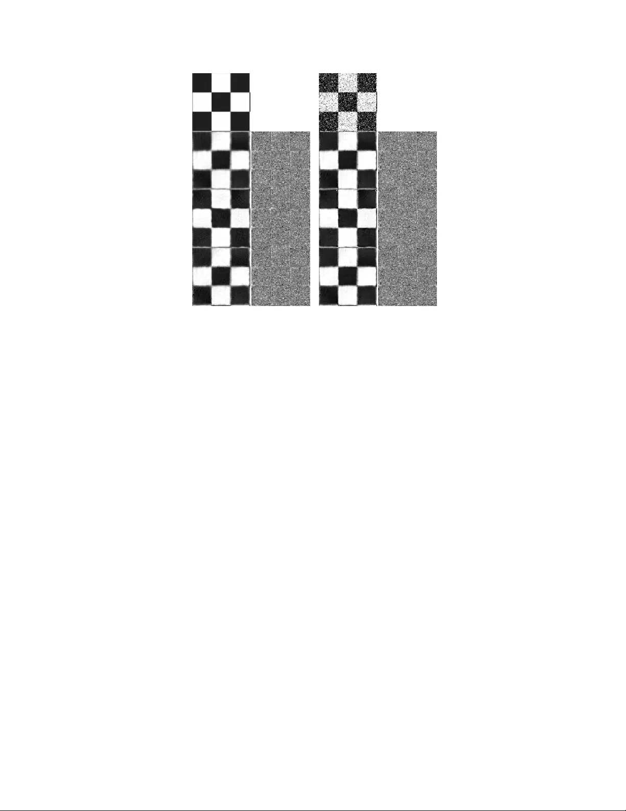
1 Probabilistic Non-Local Means Y ue W u, Brian T racey, Premkumar Natarajan and Joseph P . Noonan Abstract In this paper , we propose a so-called probabilistic non-local means (PNLM) method for image denoising. Our main contributions are: 1) we point out defects of the weight function used in the classic NLM; 2) we successfully deriv e all theoretical statistics of patch-wise differences for Gaussian noise; and 3) we employ this prior information and formulate the probabilistic weights truly reflecting the similarity between two noisy patches. The probabilistic nature of the ne w weight function also provides a theoretical basis to choose thresholds rejecting dissimilar patches for fast computations. Our simulation results indicate the PNLM outperforms the classic NLM and many NLM recent variants in terms of peak signal noise ratio (PSNR) and structural similarity (SSIM) index. Encouraging improvements are also found when we replace the NLM weights with the probabilistic weights in tested NLM variants. Index T erms Image Denoising, Non-Local Means, Probabilistic Modeling, Adaptiv e Algorithm I . I N T RO D U C T I O N Non-local means (NLM) is a popular data-adaptiv e image denoising technique introduced by Buades et al. [1], [2]. This technique is proven to be effecti ve in man y image denoising tasks. In the classic NLM, a 2D clean image x = { x l } l ∈ I defined on the spatial domain I is assumed to be contaminated by i.i.d. zero-mean Gaussian noise with an unknown variance σ 2 , i.e. y l = x l + n l , and n l ∼ N (0 , σ 2 ) . (1) where y l , x l and n l denote the noisy observ ation, the clean image pixel and the pixel noise, respecti vely . The NLM then estimates the clean pix el x l by using a weighted sum of the noisy pixels within a prescribed Y ue W u, Brian Trace y and Joseph P . Noonan are with the department of electrical and computer engineering, T ufts univ ersity , 161 College A ve, Medford, MA 02155; e-mail: ywu03@ece.tufts.edu. Premkumar Natarajan is with the Raytheon BBN technologies, 10 Moulton St., Cambridge, MA 02138. This project is supported by the T ufts subcontract to BBN on MADCA T contract (Prime Contract HR0011-08-C-004). November 27, 2024 DRAFT 2 search region S , typically a square or a rectangular re gion: b x l = P k ∈ S l w l,k y k /W l (2) where each weight is computed by quantifying the similarity between two local patches (defined as P ) around noisy pixels y l and y k as sho wn in Eq. (3), w l,k = exp  − P j ∈ P ( y l + j − y k + j ) 2 /h  (3) and the summation of all weights is denoted as W l = P k ∈ S l w l,k . (4) Although the original NLM weight [1], [2] includes a weak Gaussian smoother , the weight (3) is a simplified version with similar performance that is also widely accepted in the NLM community [3]. W ithin the NLM framework, much progress has been made in recent years. Some authors ha ve focused on fast NLM implementation [4], [5], while others have explored NLM parameter optimization [3], or hav e adjusted the NLM frame work to achie ve better performance [6]. W e notice that one shared interest of these three topics is the weight function of the NLM, which is the core of the NLM algorithm. Calculation of NLM weights is the most computationally expensi ve part of the algorithm and is related to many parameter optimization schemes. It has long been noticed that the NLM weight function is some what inadequate [7] because it tends to gi ve non-zero weights to dissimilar patches. Howe ver , the reason behind this inadequac y has not fully e xplored. In this letter, we focus on the NLM weight function and propose a new weight under a probabilistic frame work. The rest of the paper is organized as follows: Sec. II shows the defects of the NLM weights; Sec. III proposes our PNLM frame work with new probabilistic weights; Sec. IV shows simulation results; and we conclude the letter in Sec. V . I I . P RO B L E M S W I T H T H E N L M W E I G H T F U N C T I O N The NLM weight function (3) is considered as w l,k = exp( − D l,k /h 0 ) , where h 0 is a translation of the temperature parameter h in (3) and D l,k = P j ∈ P ( y l + j − y k + j ) 2 / 2 σ 2 (5) is the patch dif ference between the patches around y l and y k . In this way , (5) can be interpreted as the standard quantitativ e χ 2 test to measure the similarity of the two samples [8]. The statistical interpretation November 27, 2024 DRAFT 3 of the exponential function used in (3) is not straightforward [8], although may be possible to relate it to Gaussian kernels used in probability density estimation. Nevertheless, this exponential function giv es a larger weight to a pixel with a smaller patch difference (Fig. 1(a)). Intuitiv ely , this idea is quite reasonable, as it means that the NLM relies more on pixels with smaller patch differences. Howe ver , we demonstrate belo w that this exponential function makes the NLM weights somewhat problematic. Fig. 1: NLM weight function and the distribution of 7 × 7 patch differences. (a) the NLM weight for h = σ 2 | P | ; and (b) the distribution of disjoint patch differences. Red and green circles denotes two equal probable patch dif ferences, while are biasedly weighted in NLM. From now on, we consider D l,k as a random variable (r .v .) and assume patches around x l and x k match perfectly , i.e. P j ∈ P ( x l + j − x k + j ) 2 = 0 . (6) If they are disjoint, then D l,k ∼ χ 2 | P | , where | · | denotes the cardinality function. Fig. 1 sho ws this distribution on the right, with the corresponding NLM weight function on the left. It is clear that the NLM weight function giv es two equally probable D l,k s very different weights and that it fails to giv e the largest weight to the most probable case. For D l,k s close to its expected value, the weight errors are not too large because the corresponding region in the exponential curve is almost linear with a moderate slope. Ho wev er, for D l,k s f ar a way from its e xpected v alue, weight errors are very large because the NLM function tends to gi ve nonzero weights to these highly improbable cases, so weight errors grow quickly . In practice, correcting ov er-weighted weights has been shown to improv e NLM performance. For example, the center pixel weight (CPW) in NLM is unitary and thus over -weights center pixels. [9], [10] report noticeable improv ement just by tuning these over -weighted CPWs. November 27, 2024 DRAFT 4 I I I . P RO B A B I L I S T I C N O N - L O C A L M E A N S Instead of including the e xponential function in weighting pixels, we propose the follo wing probabilistic weight w l,k = f l,k  b D l,k /ρ 2  (7) where f l,k ( · ) is the theoretical probability density function (p.d.f.) of the r .v . D l,k , b D l,k is the patch dif ference using estimated variance b σ 2 in (5), and ρ is a tuning parameter . This weight function then can be interpreted as the probability of seeing a noisy patch difference when we kno w the two clean patches match perfectly . A. Theor etical Distribution of P atch-wise Distance Pretend we kno w the true noise v ariance σ 2 (later we will show this knowledge is unnecessary). Our goal is to deriv e the theoretical p.d.f. of the patch dif ference when the two clean patches around pixel x l and x k are perfectly matching (see (6)). T o do so, we denote the pixel distance d l,k as d l,k = ( y l − y k ) 2 / 2 σ 2 (8) and thus we ha ve D l,k of the form that D l,k = P j ∈ P d l + j,k + j . (9) Because two patches are perfectly matching and noise is i.i.d., for all j ∈ P we hav e d l + j,k + j = ( n l + j − n k + j ) 2 2 σ 2 ∼ χ 2 1 . If all d l + j,k + j s are i.i.d., then we have D l,k ∼ χ 2 | P | , whose mean is | P | and variance is 2 | P | . Ho wev er, the i.i.d. assumption does not hold when the two patches overlap, as is the case for many pairs of patches. Fortunately , it is known that such a summed correlated χ 2 distribution can be well approximated [11] as follo ws, D l,k ∼ γ k χ 2 η k (10) where parameters γ k and η k can be determined by the first two cumulants of D l,k [11] as sho wn below . γ k = v ar [ D l,k ] / (2 E [ D l,k ]) (11) η k = E [ D l,k ] /γ k (12) November 27, 2024 DRAFT 5 The cumulant E [ D l,k ] is straightforward to find, and it is E [ D l,k ] = P j ∈ P E [ d l + j,k + j ] = | P | . (13) W ith regards to var [ D l,k ] , the follo wing identity always holds v ar [ D l,k ] = P i,j ∈ P cov [ d l + i,k + i , d l + j,k + j ] (14) where the cov ariance can be written as follo ws. cov [ d l + i,k + i , d l + j,k + j ] = E [ d l + i,k + i d l + j,k + j ] − µ 2 d l,k (15) This equation compares two pairs of r .v .s, N i l,k = { n l + i , n k + i } and N j l,k = { n l + j , n k + j } , of which 0, 1 or 2 may be repeated. Thus, E [ d l + i,k + i d l + j,k + j ] =          3 , if | N i l,k ∩ N j l,k | = 2 1 . 5 , if | N i l,k ∩ N j l,k | = 1 1 , if | N i l,k ∩ N j l,k | = 0 (16) found as E [ d l + i,k + i d l + j,k + j ] measures kurtosis if both pixels are repeated; pixels are i.i.d. if distinct; and by expanding terms if one pixel is repeated. This implies that cov [ d l + i,k + i d l + j,k + j ] =          2 , if | N i l,k ∩ N j l,k | = 2 0 . 5 , if | N i l,k ∩ N j l,k | = 1 0 , if | N i l,k ∩ N j l,k | = 0 . (17) v ar [ D l,k ] is thus dependent on the number of terms for which | N i l,k ∩ N j l,k | = 2 and for which | N i l,k ∩ N j l,k | = 1 . Case | N i l,k ∩ N j l,k | = 2 happens only when i = j , and so the number of ov erlapped pixels is | P | . Case | N i l,k ∩ N j l,k | = 1 happens only when two patches overlap, and the corresponding number is the same as the number of ov erlapping pixels. Letting O l,k be the set of overlapping pixels, var [ D l,k ] can be written as v ar [ D l,k ] = 2 | P | + | O l,k | (18) and is known once k is gi ven. As a result, γ k and η k in (11) and (12) can be determined, implying the p.d.f. of D l,k is f l,k ( D ) = χ 2 η k ( D /γ k ) = ( D /γ k ) η k / 2 − 1 exp( − D / 2 γ k ) 2 η k / 2 Γ( η k / 2) . (19) November 27, 2024 DRAFT 6 The different spatial relationships of patch pairs imply different | O l,k | , thus causing different var [ D l,k ] , γ k , and finally p.d.f. f l,k . This conclusion means that NLM weights calculated without considering spatial correlations are inadequate. f l,k also provides a natural criterion for speeding computation by rejecting over -dissimilar patches at an early stage (see similar usage in [4]). Thresholds can be set by finding critical v alues D ∗ + α and D ∗− α under a prescribed significance level α such that Pr ( D ∗− α ≤ D ≤ D ∗ + α | f l,k ) = α. (20) B. P arameter s Discussions Abov e we did not use f l,k ( b D l,k ) as our weight function, but instead used f l,k ( b D l,k /ρ 2 ) . The parameter ρ 2 provides a way to adjust our probabilistic model when an estimated variance b σ 2 is used instead of the true σ 2 . When ρ 2 = σ 2 / b σ 2 (21) reflects the ratio of the true noise variance to the estimated one, all pre vious deri vations hold. Thus b d l,k = ( y l − y k ) 2 / 2 b σ 2 = ρ 2 ( y l − y k ) 2 / 2 σ 2 ∼ χ 2 ρ 2 (22) indicating that E [ b D l,k ] = ρ 2 | P | and var [ b D l,k ] = ρ 4 (2 | P | + | O l,k | ) . Further, this implies that the actual parameters used are b γ k = ρ 2 γ k and b η k = η k . Finally , these results lead to b f l,k ( b D ) = χ 2 b η k ( b D / b γ k ) = χ 2 η k ( b D / ( ρ 2 γ k )) = f l,k ( b D /ρ 2 ) which is the weight function given in (7). The raw probabilistic CPW w l,l = f l,k (0) ≈ 0 under -weights a noisy center pixel. A more plausible CPW is w l,l = χ 2 | P | ( | P | ) . (23) which is the same as the weight of the most probable case. This CPW is used for the rest of the letter . I V . S I M U L A T I O N R E S U LT S All of the following simulations are done under the MA TLAB r2012b environment. Our two goals are 1) to show that the deri ved p.d.f. f l,k in (19) closely approximates its true p.d.f.; and 2) to confirm the superiority of the proposed probabilistic weights and PNLM. November 27, 2024 DRAFT 7 Fig. 2 shows the var [ D l,k ] map for a 7 × 7 search region S l with 3 × 3 patches and the six typical theoret- ical p.d.f.s f l,k , plotted with the corresponding sample distributions estimated from 100,000 realizations. It is noticeable that the var [ D l,k ] map is location-dependent and isotropic with one of the six theoretical v alues { 18,19,20,21,22,24 } . The more pixels ov erlap, the larger var [ D l,k ] is, implying a smaller peak on its p.d.f. It is clear that the predicted p.d.f.s are v ery close to those estimated from a large number of samples. Since it is clear that the accuracy of the f l,k approximation degrades as correlation increases, the approximation accuracy of the most-overlapped cases can be used to characterize the worst-case accuracy . For each combination of search region S l and patch size P , there are four possible k s that attain the maximum correlation, all of which are one pixel away from the center pix el (see examples for k =18, 24, 26, and 32 on Fig. 2-(a)). In T able I, we report the av eraged P-values of goodness of fit tests for the most correlated f l,k s, where each P-value is the av eraged from P-values of the four most correlated f l,k s. Because all observ ed P-values are abov e 5%, we say the approximated theoretical p.d.f. (19) gi ves satisfactory predictions, so these p.d.f.s can reliably be used to quantify patch similarities. T ABLE I: A veraged P-v alues of goodness of fit tests for the observed sample distributions. Search Region Size 7 11 15 21 29 Patch Size 3 0.5853 0.6865 0.2252 0.1001 0.5612 5 0.2675 0.3125 0.3374 0.5746 0.3501 7 0.3967 0.4659 0.1545 0.2645 0.4282 9 0.4741 0.8665 0.5233 0.3405 0.6582 In the follo wing simulation, we compare the three pairs of NLM and PNLM algorithms, namely 1) the classic NLM and the proposed PNLM, 2) the classic NLM with the James-Stein Shrinkage (JSNLM) [10] and the proposed PNLM with the James-Stein Shrinkage (PSJNLM), and 3)the nonlocal median with the classic weights (NLEM) [6] and the nonlocal median with the probabilistic weights (PNLEM). The only difference between the two algorithm in each pair is the weight function. W ith regards to the parameter settings, we use patch size 7 and search region size 21 for all methods. For the temperature parameter h in NLMs, we use h = | P | σ 2 , which is nearly optimal and suggested in [3]. For ρ in PNLMs, we use ρ = 1 . T o quantify the quality of a denoised method, we compute the av erage PSNR [3] and SSIM [12] scores from 10 realizations for each method and each noise le vel. These results are reported in T able II. From T able II, it is clear that 1) the proposed PNLM method outperforms the NLM method and those recent variants like NLEM and JSNLM; and 2) by replacing the NLM weight with the ne w proposed probabilistic one, both NLEM and JSNLM are improved in terms of higher PSNR/SSIM scores. Fig.3 November 27, 2024 DRAFT 8 (a) (b) (c) (d) (e) (f) (g) Fig. 2: Theoretical and estimated p.d.f. f l,k s for 7 × 7 search region and 3 × 3 patches. (a) theoretical var [ D l,k ] map (white indices indicates k s in S l ). (b)-(g) theoretical (red dash lines) and estimated (blue bars) p.d.f. f l,k s for k = 8 (var [ D l, 8 ] =18 ), k = 9 (v ar [ D l, 9 ] = 19 ), k = 10 (var [ D l, 10 ] = 20 ), k = 11 (var [ D l, 11 ] = 21 ), k = 17 (v ar [ D l, 17 ] = 22 ) and k = 18 (var [ D l, 18 ] = 24 ), respectiv ely . gi ves example denoising results and method noise images of the NLM and PNLM algorithms. These results show that the effecti veness of the new proposed probabilistic weight and the superiority of the PNLM frame work. V . C O N C L U S I O N In this letter , we pointed out the insuf ficiency of the NLM weights and showed a ne w promising PNLM frame work, whose weights better reflect patch similarities. The proposed PNLM framework connects the denoising process and the noise type and thus is meaningful for denoising other types of noise. As long as a noise p.d.f. is kno wn, we can estimate f l,k correspondingly . In this way , a univ ersal denoising November 27, 2024 DRAFT 9 T ABLE II: Performance comparisons for NLM and PNLM methods PSNR(dB) \ σ 10 20 30 40 50 60 70 80 90 100 cameraman NLM 32.57 28.92 26.98 24.98 23.52 22.52 21.84 21.24 20.82 20.44 PNLM 32.47 29.08 27.44 26.26 25.19 24.13 23.26 22.44 21.84 21.31 NLEM 32.66 28.90 26.63 24.78 23.35 22.16 21.78 21.31 20.95 20.55 PNLEM 33.06 29.42 27.36 25.72 24.90 23.87 23.11 22.28 21.73 21.13 JSNLM 32.64 29.01 27.13 25.46 24.12 23.10 22.33 21.61 21.09 20.63 PSJNLM 32.21 29.08 27.45 26.16 25.07 24.05 23.20 22.40 21.77 21.23 house NLM 34.08 31.30 28.79 26.88 25.62 24.66 23.85 23.31 22.90 22.45 PNLM 34.92 32.40 30.48 28.70 27.25 26.14 24.98 24.17 23.57 22.98 NLEM 34.30 30.43 27.80 26.53 25.51 24.88 24.13 23.52 22.92 22.43 PNLEM 34.56 31.97 30.24 28.64 27.07 26.11 24.90 24.14 23.38 22.94 JSNLM 34.62 31.70 29.29 27.30 25.94 24.87 23.98 23.35 22.86 22.37 PSJNLM 34.81 32.38 30.36 28.58 27.11 25.89 24.82 23.99 23.36 22.75 lenna NLM 33.74 30.91 28.72 27.14 26.03 25.13 24.42 23.88 23.44 23.03 PNLM 34.59 32.07 30.17 28.58 27.32 26.23 25.33 24.59 23.98 23.43 NLEM 33.56 30.00 28.41 27.30 26.47 25.65 25.05 24.29 23.64 23.12 PNLEM 33.78 31.21 29.64 28.32 27.26 26.28 25.58 24.80 24.20 23.69 JSNLM 34.38 31.41 29.21 27.49 26.26 25.26 24.47 23.85 23.33 22.86 PSJNLM 34.72 32.07 30.09 28.48 27.20 26.07 25.15 24.38 23.74 23.15 check er NLM 39.04 33.80 30.95 28.94 27.37 25.94 24.45 23.25 21.84 20.87 PNLM 40.34 35.17 32.31 30.26 28.38 26.71 25.37 24.50 23.29 22.76 NLEM 39.68 34.13 30.90 28.94 27.07 25.62 24.59 23.54 22.66 22.09 PNLEM 39.72 34.49 31.25 29.18 27.15 25.77 24.68 23.78 22.93 22.52 JSNLM 39.03 33.79 30.93 28.93 27.35 25.91 24.42 23.22 21.81 20.84 PSJNLM 34.64 30.86 31.23 29.73 27.95 26.39 25.08 24.25 23.10 22.60 SSIM(%) \ σ 10 20 30 40 50 60 70 80 90 100 cameraman NLM 91.08 82.92 78.50 73.87 68.97 64.18 59.78 55.58 51.87 48.69 PNLM 91.64 84.65 80.23 76.61 73.26 69.72 66.18 62.72 59.45 56.60 NLEM 88.68 80.24 72.53 64.98 59.15 53.04 48.67 43.96 40.45 35.95 PNLEM 91.16 83.22 78.13 73.31 68.89 63.11 58.90 54.51 50.54 46.18 JSNLM 91.23 84.32 78.91 73.63 68.74 64.01 59.62 55.34 51.36 48.23 PSJNLM 89.69 84.04 79.29 74.97 71.01 66.98 63.13 59.30 55.61 52.82 house NLM 87.63 83.77 79.88 75.11 70.63 66.34 62.16 58.30 54.86 51.40 PNLM 89.38 85.00 81.72 78.18 74.70 71.05 67.43 63.99 60.81 58.05 NLEM 88.06 81.79 75.43 69.11 63.09 57.09 51.09 45.81 41.19 37.04 PNLEM 89.17 84.11 79.92 75.17 70.40 65.40 59.92 54.59 49.58 46.80 JSNLM 89.12 84.14 79.54 74.52 69.78 65.19 60.80 56.94 53.33 49.86 PSJNLM 89.34 84.57 80.64 76.45 72.35 68.03 63.80 60.11 56.49 53.34 lenna NLM 87.86 83.98 79.39 74.90 70.72 66.72 62.87 59.23 55.82 52.59 PNLM 89.69 85.00 81.18 77.56 74.16 70.78 67.57 64.51 61.44 58.81 NLEM 88.21 81.19 75.44 69.48 63.71 57.57 52.22 46.92 42.29 38.54 PNLEM 89.56 84.02 79.03 74.05 69.42 64.64 60.09 55.85 51.87 48.25 JSNLM 89.37 83.94 79.16 74.48 69.95 65.67 61.61 57.86 54.32 50.99 PSJNLM 89.75 84.64 80.21 76.00 71.93 67.97 64.16 60.70 57.23 54.11 check er NLM 99.01 97.38 95.35 93.23 90.75 87.94 84.22 80.76 76.31 72.00 PNLM 99.33 98.32 97.03 95.68 93.82 91.79 89.48 87.61 84.87 82.95 NLEM 99.10 97.67 95.46 92.65 89.20 85.12 81.90 78.73 74.26 71.71 PNLEM 99.22 97.99 96.03 94.26 91.83 88.85 85.91 83.16 79.38 77.35 JSNLM 99.00 97.34 95.24 93.11 90.53 87.59 83.79 80.23 75.65 71.18 PSJNLM 94.25 92.72 95.09 93.74 91.66 89.53 86.86 84.83 82.02 80.14 frame work (see example [13]) for multiple types of known noises and mixed noises may be developed. In addition, the proposed PNLM can also be extended to capture non i.i.d. noises, because one can easily to replace the p.d.f. of patch difference f l,k with more general forms. F or example, for Gaussian noises with changing v ariance, f l,k ( D | σ 2 ) Pr ( σ 2 ) can be used in place of f l,k ( D ) . The proposed PNLM also provides a theoretical basis to quantify patch similarities, so Eq. (20) can be used in other ways other than early termination. For example, the critical values predicted by f l,k can also be used as thresholds to reject or accept a patch in the first stage of BM3D [14]. This choice pro vides a theoretically-based November 27, 2024 DRAFT 10 (a) (b) (c) (d) (e) (f) (g) (h) Fig. 3: NLM and PNLM denoising results for σ = 80 (cropped and enlarged from results of image check er ). (a) clean image; (b) noisy observation; (c) to (h): denoising results and method noise images of NLM, PNLM, NLEM, PNLEM, JSNLM, and PJSNLM, respectiv ely . alternati ve to the empirical hard thresholds in BM3D ( i.e. τ match in Eq. (2) of [14]). In our initial tests, we also see a performance improvement after using the probabilistic thresholds. R E F E R E N C E S [1] A. Buades, B. Coll, and J. Morel, “ A re view of image denoising algorithms, with a ne w one, ” Multiscale Modeling & Simulation , vol. 4, no. 2, pp. 490–530, 2005. [2] A. Buades, B. Coll, and J.-M. Morel, “ A non-local algorithm for image denoising, ” in IEEE Computer Society Confer ence on Computer V ision and P attern Recognition , vol. 2, june 2005, pp. 60 – 65 vol. 2. [3] D. V an De V ille and M. K ocher , “Sure-based non-local means, ” IEEE Signal Pr ocessing Letters , vol. 16, no. 11, pp. 973 –976, nov . 2009. [4] R. V ignesh, B. T . Oh, and C.-C. Kuo, “Fast non-local means (nlm) computation with probabilistic early termination, ” Signal Pr ocessing Letters, IEEE , vol. 17, no. 3, pp. 277–280, 2010. [5] K. Chaudhury , “ Acceleration of the shiftable o(1) algorithm for bilateral filtering and non-local means, ” IEEE T ransactions on Image Pr ocessing , vol. PP , no. 99, p. 1, 2012. [6] K. N. Chaudhury and A. Singer , “Non-local euclidean medians, ” IEEE Signal Pr ocessing Letters , vol. 19, no. 11, pp. 745 –748, nov . 2012. [7] V . Duval, J. Aujol, and Y . Gousseau, “ A bias-variance approach for the nonlocal means, ” SIAM Journal on Imaging Sciences , vol. 4, no. 2, pp. 760–788, 2011. [8] N. Thacker , J. Manjon, and P . Bromile y , “Statistical interpretation of non-local means, ” Computer V ision, IET , vol. 4, no. 3, pp. 162–172, 2010. [9] J. Salmon, “On two parameters for denoising with non-local means, ” IEEE Signal Pr ocessing Letters , vol. 17, no. 3, pp. 269 –272, mar . 2010. November 27, 2024 DRAFT 11 [10] Y . W u, B. T racey , N. P ., and J. Noonan, “James-stein type center pixel weights for non-local means image denoising, ” IEEE Signal Pr ocessing Letters , vol. 17, no. 3, pp. 277 –280, Jan. 2013. [11] L.-L. Chuang and Y .-S. Shih, “ Approximated distributions of the weighted sum of correlated chi-squared random variables, ” Journal of Statistical Planning and Infer ence , vol. 142, no. 2, pp. 457–472, 2012. [12] Z. W ang, A. Bovik, H. Sheikh, and E. Simoncelli, “Image quality assessment: From error visibility to structural similarity , ” IEEE T ranscations on Image Pr ocessing , vol. 13, no. 4, pp. 600–612, 2004. [13] Z. Sun and S. Chen, “Modifying nl-means to a universal filter , ” Optics Communications , 2012. [14] K. Dabo v , A. Foi, V . Katkovnik, and K. Egiazarian, “Image denoising with block-matching and 3 d filtering, ” in Pr oceedings of SPIE , vol. 6064, 2006, pp. 354–365. November 27, 2024 DRAFT