An algorithm to compute the power of Monte Carlo tests with guaranteed precision

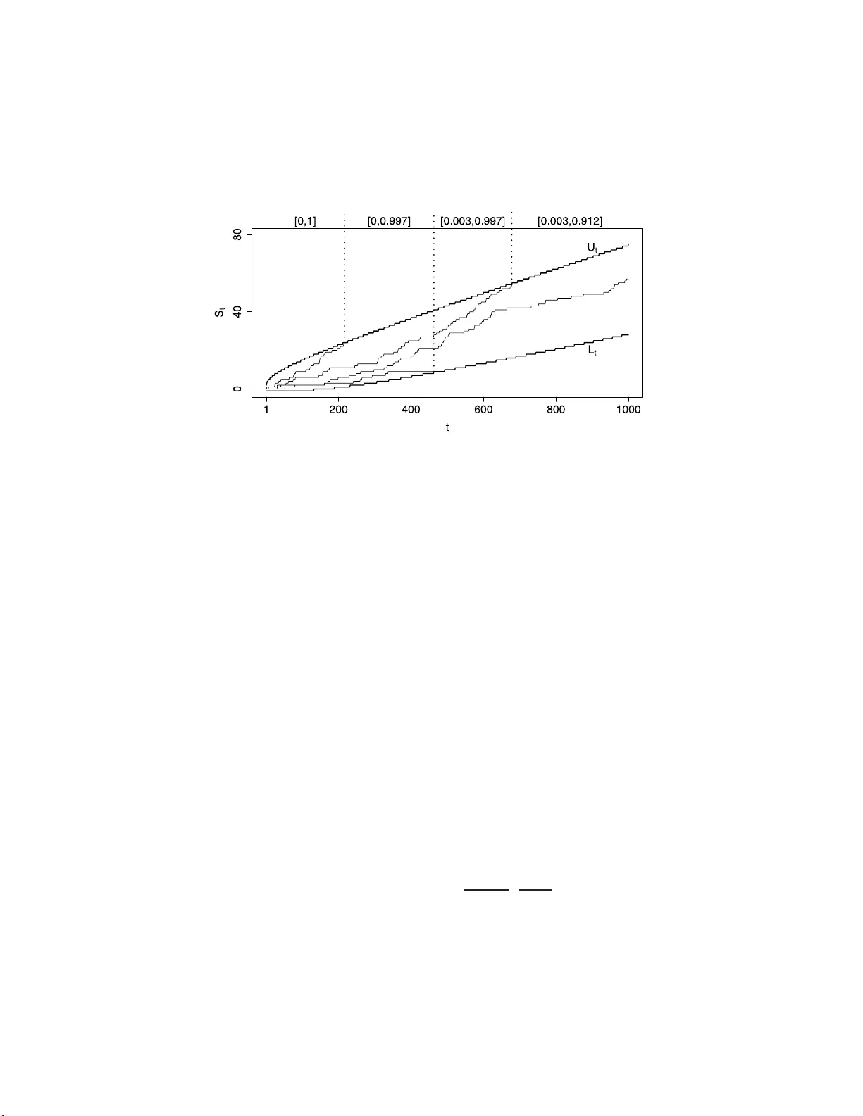
The Annals of Statistics 2013, V ol. 41, No. 1, 125–142 DOI: 10.1214 /12-AOS1076 c  Institute of Mathematical Statistics , 2 013 AN ALGORITHM TO COMPUTE THE PO WER OF MONTE CARLO TESTS WITH GUARANTEED PRECISION 1 By Axel Gandy and P a trick R ubin-Delanc hy Imp erial Col le ge L ondon and University of Bristol This article presents an algorithm that generates a conserv ative confidence in terv al of a sp ecified length and cov erage probability for the p ow er of a Monte Carlo test (suc h as a b o otstrap or p ermuta- tion test). I t is th e fi rst method that achiev es this aim for almost any Monte Carlo test. Previous research h as focused on obtaining as accurate a result as p ossible for a fixed computational effort, without providing a guaranteed precision in the a b ov e sense. The algorithm w e prop ose do es n ot hav e a fixed effort and ru ns u ntil a confi dence interv al with a user-sp ecified length and cov erage p rob ab ility can b e constructed. W e show that the ex p ected effort required by the algorithm is fi nite in most cases of practical interest, including situ- ations where the distribution of th e p -val ue is absolutely contin uous or discrete with finite supp ort. The algorithm is implemented in the R-pack age simctest , av ailable on CRAN. 1. In tro duction. Let p b e a random v ariable taking v alues in [0 , 1] w ith unknown cumulativ e distribution fun ction (CDF) F . F or some α ∈ (0 , 1), w e w an t to appro ximate β = F ( α ) by Mon te Carlo sim ulation. Assu me that w e cannot samp le from F directly , b ut that it is p ossible to generate a collec- tion of random v ariables ( X i j : i ∈ N , j ∈ N ), where X i 1 , X i 2 , . . . ∼ Bernoulli ( p i ) indep end en tly and p 1 , p 2 , . . . are unobserved in dep end en t copies of p , that is, p 1 , p 2 , . . . ∼ F ind ep endently . This problem comes ab out when computing the p o w er or lev el of a Mont e Carlo test, suc h as a b o otstrap or p erm utation test, or in general a test that rejects on the basis of simulat ions un der the (p oten tially estimated) n ull hypothesis. I n this con text, p is the (random) p -v alue, α the nominal lev el of the test and β its p o w er. In this situation X i 1 , X i 2 , . . . are generated as follo ws: simulate a dataset (thus implicitly generating p i ), compute the Received March 2012; revised August 2012. 1 Supp orted by EPSR C Grant EP/H0401 02/1. AMS 2000 subje ct classific ations. Primary 62-04, 62L12; secondary 62L15, 62F40. Key wor ds and phr ases. Monte Carlo testing, significance test, p o wer, algorithm. This is an electronic r e print of the origina l article published b y the Institute of Mathematical Statistics in The Annals of Statist ics , 2013, V ol. 41 , No . 1 , 125 –142 . This reprint differs from the orig inal in pa gination and t yp ogr aphic detail. 1 2 A. GANDY AN D P . RUBIN-DELANCHY observ ed test statistic and then , for j = 1 , 2 , . . . , use a samp ling tec hnique (suc h as b o otstrapping or p erm utation) on the observ ed dataset to get a (re)sampled realizatio n of the test statistic und er the null hypothesis. Define X i j as the indicator th at the (re)sampled test statistic is at least as extreme as the observ ed test statistic. A t ypical approac h is to c ho ose N , M ∈ N = { 1 , 2 , . . . } and estimate β b y ˆ β na ¨ ıve = 1 N N X i =1 I " 1 M M X j =1 X i j ! ≤ α # , where I is the indicator function. A problem of this appr oac h is that the bias of ˆ β na ¨ ıve is un kno wn. F or example, using [ 1 ], equation (2), it can b e shown that no matter how large N and M are c hosen, sup P ∈P | E ˆ β na ¨ ıve − β | ≥ 0 . 5 , where P is th e set of all p r obabilit y d istributions on [0 , 1]. Better b ou n ds are av aila ble under the assum ption that E ˆ β na ¨ ıve is conca ve in α , see [ 3 ], Sec- tion 4.2.5. Ho we ver, this would u sually not b e known in a giv en application. More adv anced estimat ion metho d s ha ve b een p rop osed. F or instance, Oden [ 10 ] h as inv estigated h o w to c ho ose th e relativ e sizes of N (con trolling the v ariance) and M (con trolling the bias), to minimize the total estimation error for certain d istr ibutions of p . [ 1 ] p artially correct the bias by extrap o- lation. Ho w ev er, existing pro cedures do not pro vide a formal, fin ite-sample guar- an tee on the accuracy of ˆ β f or a general test. This is partly b ecause the problem has alwa ys b een ap p roac hed with the principle of fin ding as accu- rate an estimate as p ossible for a fi xed computational effort. W e approac h the pr oblem with the p riorities r ev ersed: we make an exact probabilistic statemen t ab out the result, allo wing the computational effort to b e r andom. The algorithm th at we prop ose is guaran teed to p r o vide a conserv ativ e confidence interv al (CI) for β of a giv en co verage p robabilit y . This interv al will, after a finite exp ected num b er of samples, r eac h any desired length, pro vided that F is H¨ older contin uous in a neighborh o o d of α with exp onen t ξ > 0. Th is is satisfied if, for example, in a n eigh b orho o d of α , p is absolutely con tin uous with resp ect to Leb esgue measure w ith b ounded d ensit y . In this case ξ = 1. F or practical use, the inner w orkings of the algorithm can b e ignored. Users only need to provide the required precision (maximum CI length and minim um co verage pr obabilit y) and a mechanism for generating the X i j . Th e algorithm is implemen ted in the R-pac k age simctest , a v ailable on C RAN. The article is structured as follo ws. In Section 2 w e describ e the basic algorithm. Theorem 2.1 demons trates that, und er v ery mild conditions, the COMPUTING THE POWER OF MONTE CARLO TESTS 3 algorithm terminates in finite exp ected time. Sections 3 and 4 p r esen t addi- tional metho dology to red u ce the computational effort, some d etails of wh ic h are in s upplementa ry material [ 6 ]. S ection 5 conta ins a simulation study . In Section 6 , w e suggest an adaptive rule wh ic h ensures that the computational effort is only h igh if the estimate is in a region of interest. In Section 7 we demonstrate the use of our algorithm on a simple p ermutat ion test example. Pro ofs and auxiliary lemmas are in the App end ix . Within these, Lemma A.1 confirms an observ ation made in [ 5 ], main text page 1507 and Figure 4, ab out the distance b et wee n certain stopp ing b oun daries. 2. The basic algorithm. 2.1. D escription. W e use th e notation int ro d uced in th e fir st paragraph of the In tro d u ction . F or ev ery i ∈ N , we call the Bernoulli sequence ( X i j ) j ∈ N a str e am . The algorithm will use a fixed num b er N of these streams. F or eac h str eam i , our algorithm aims to decide if p i ≤ α or if p i > α . W e use the sequen tial algorithm of [ 5 ] for this purp ose. T o simp lify notation, we often drop the stream index i when referrin g to a generic str eam; f or example, we write X j , p instead of X i j , p i . F urthermore, w e use a sub script to ind icate the pr obabilit y distrib ution of such a stream conditional on a sp ecific v alue of p , that is, P q ( · ) = P( ·| p = q ) for some q ∈ [0 , 1]. The pro cedu r e in [ 5 ] defin es t w o deterministic sequences, an upp er b ound - ary ( U t : t ∈ N ) and a lo we r b ound ary ( L t : t ∈ N ). While the partial sum S t = P t j =1 X j has hit neither b oundary , the stream is unr esolve d . The p ro- cedure terminates at the h itting time τ = in f { t : S t ≥ U t or S t ≤ L t } . If the upp er b oundary is hit, w e decide p > α and rep ort a ne gative outc ome ( p is n ot significan t at lev el α ). If the low er b oun dary is hit we decide p ≤ α and rep ort a p ositive outc ome ( p is s ignifi can t at level α ). The b oun d aries are constructed to give a d esired uniform b ound ε > 0 on the pr obabilit y of a wrong decision, that is, P p ( S τ = U τ ) ≤ ε for p ≤ α, (2.1) P p ( S τ = L τ ) ≤ ε for p > α. Figure 1 shows an example of U t and L t with ε = 0 . 01 and α = 0 . 05. T o b e more p r ecise, the b oun daries are constructed recursively u sing a sp ending se qu enc e ( ε t ) with 0 ≤ ε t ր ε as t → ∞ . The sp endin g sequence go verns ho w quickly th e error p robabilit y ε is sp en t, guarant eeing P p ( S τ = U τ , τ ≤ t ) ≤ ε t for p ≤ α, P p ( S τ = L τ , τ ≤ t ) ≤ ε t for p > α. The precise recursive construction is giv en in ( A.1 ), in the App endix . 4 A. GANDY AN D P . RUBIN-DELANCHY Fig. 1. Confidenc e intervals gener ate d by the al gorithm using N = 4 , ε = 0 . 01 , α = 0 . 0 5 , ε t = εt/ (1000 + t ) and γ = 0 . 05 . Our algo rithm runs N streams in parallel unt il enough ha v e b een resolv ed to meet the required precision. More formally , it op erates as follo ws: Algorithm 1 (Basic algorithm). L et t = 0 ; R 0 = 0 ; A 0 = 0 ; U 0 = { 1 , . . . , N } , S 1 0 = 0 , . . . , S N 0 = 0 while | I ( R t , A t , |U t | ; γ ) | > ∆ L et t = t + 1 , R t = R t − 1 , A t = A t − 1 , U t = U t − 1 for i ∈ U t L et S i t = S i t − 1 + X i t If S i t ≥ U t let A t = A t + 1 , U t = U t \ { i } If S i t ≤ L t let R t = R t + 1 , U t = U t \ { i } R ep ort I ( R t , A t , |U t | ; γ ) as c onfidenc e i nterval for β . U t is a set con taining the indices of unresolv ed streams at time t . | · | denotes the size of fin ite sets as wel l as th e length of interv als. R t and A t coun t, resp ectiv ely , the num b er of p ositiv e and negativ e outcomes. I ( R t , A t , |U t | ; γ ) is a conserv ativ e confidence in terv al for β based on R t , A t and |U t | . I t is constructed as follo ws. Because of ( 2.1 ), the probab ility that a stream has a p ositiv e outcome is in the interv al [(1 − ε ) β , (1 − ε ) β + ε ]. Therefore, if all streams were resolv ed, the follo wing in terv al would b e a conserv ativ e confiden ce interv al for β with co v erage pr obabilit y 1 − γ : I ∞ = I ∞ ( R ∞ , A ∞ ; γ ) =  β ∗ − − ε 1 − ε , β ∗ + 1 − ε  , where R ∞ ( A ∞ ) denotes the num b er of p ositiv e (negativ e) outcomes and [ β ∗ − , β ∗ + ] is th e C lopp er–Pe arson confid ence in terv al [ 2 ] with co ve rage prob- abilit y 1 − γ for the success probab ility of a Binomial random v ariable ob- serv ed to b e R ∞ after R ∞ + A ∞ trials. COMPUTING THE POWER OF MONTE CARLO TESTS 5 The subscript in I ∞ represent s that this is the in terv al th at w ould b e obtained by our algorithm if it were r un until all streams we re resolv ed. T o obtain a conserv ativ e confidence in terv al I t while there are unresolv ed streams, we tak e th e un ion of all confi dence inte rv als that could b e obtained after observing the outcomes of the remaining str eams, th at is, w e let I t = I ( R t , A t , |U t | ; γ ) where I ( r , a, u ; γ ) = r + u [ r ∞ = r I ∞ ( r ∞ , r + a + u − r ∞ ; γ ) . (2.2) By construction, I 1 ⊇ I 2 ⊇ · · · ⊇ I ∞ and P[ β ∈ I 1 ∩ · · · ∩ β ∈ I t ∩ · · · ∩ β ∈ I ∞ ] ≥ 1 − γ . Figure 1 illustrates the algorithm in a to y examp le with only N = 4 streams. The thin lines depict the 4 corresp onding p artial su m s equences, S i t . When S i t hits one of the b ound aries the str eam is stopp ed, causing a re- traction of the confidence inte rv al for β (ann otated at the top of the graph). 2.2. E xp e cte d time. A simpler algorithm than Algorithm 1 wo uld b e to run N s treams until all are resolv ed. N can b e c hosen suc h that the CI length is at most ∆ f or all outcomes. Ho w ev er, this algorithm is unusable in practice as it typica lly requir es an in finite exp ected effort. Indeed, from [ 5 ], page 1506, if the CDF F of p h as a nonzero deriv ativ e at α , a ve ry common case, then E[ τ i ] = ∞ , w here τ i denotes the hitting time of th e i th str eam. This make s the ov erall exp ected effort infin ite. W e no w sho w that with our alg orithm w e can choose N and ( ε t ) suc h that the exp ected effort is finite. Th e key is to make N large enough that not all str eams hav e to b e r esolv ed . The effort of Algorithm 1 , as measured b y the num b er of X i t used, is e = N X i =1 min { τ i , τ ( N − k ) } , (2.3) where k is the n u m b er of unresolv ed streams when the algorithm fin ishes and τ (1) ≤ · · · ≤ τ ( N ) denote the order statistics of τ 1 , . . . , τ N . By c ho osing N large enough and ε small enough, w e ca n ensure k ≥ κ for an y giv en κ ≥ 1. T h e effort is th en b ounded ab o v e by τ ( N − κ ) N . Thus to ensure that E[ e ] is fi nite, it suffi ces to prov e E[ τ ( N − κ ) ] < ∞ for some κ . Th e follo w in g theorem shows that in many cases κ can b e tak en as small as 2. Theorem 2.1. Supp ose tha t ε ≤ 1 / 4 and ther e e xi st c onstants λ > 0 , q > 1 and T ∈ N such that ε t − ε t − 1 ≥ λt − q for al l t ≥ T . F urther, supp ose that in a neighb orho o d of α the CDF F of p is H ¨ o lder c ontinuous with exp onent ξ . Then E[ τ ( i ) ] < ∞ for i ≤ N − ⌊ 2 /ξ ⌋ . In p articular, if ξ = 1 (the CDF is Lipschitz c ontinuous in a nei ghb orho o d of α ), then E[ τ ( N − 2) ] < ∞ . 6 A. GANDY AN D P . RUBIN-DELANCHY F is H¨ older con tin uous with exp onent ξ in a n eigh b orho o d of α if there exists an op en interv al U cont aining α for wh ic h there exists a c > 0 such that for all x, y ∈ U , | F ( x ) − F ( y ) | ≤ c | x − y | ξ . The conditions on ε and ( ε t ) are, for example, satisfied by ε t = εt/ (1000 + t ) and an y ε ≤ 1 / 4 with λ = 1 and q = 2 . Th is sp endin g sequence ( ε t ) is the default sp ending sequence in the R-pac k age simctest . The conditions on F are mild. F or example, if F h as a b ounded density in a neigh b orho o d of α , then ξ = 1. If the distribu tion of p is discrete and has fin ite s u pp ort (e.g., in a p erm utation test), then ξ = 1 if P [ p = α ] = 0 . Otherwise, it is in p rinciple p ossible to find α ′ > α suc h that β = P[ p ≤ α ] = P[ p ≤ α ′ ] , P[ p = α ′ ] = 0 . Applying the algorithm to α ′ instead of α , w e again ha ve ξ = 1. Henceforw ard the conditions of Theorem 2.1 are assumed to b e satis- fied with ξ = 1. The algorithm will meet the u ser-sp ecified p r ecision re- quirement s with a finite exp ected effort if it will terminate b y time τ ( N − 2) with probability one, or if P[ |I τ ( N − 2) | > ∆] = 0. As can b e v erified, with N − 2 of N streams resolv ed the largest p ossible C I length occur s when there are ⌊ ( N − 2) / 2 ⌋ p ositiv e outcomes. N m ust therefore satisfy | I ( ⌊ ( N − 2) / 2 ⌋ , ⌈ ( N − 2) / 2 ⌉ , 2; γ ) | ≤ ∆. W e shall call the minimal such N the b lind minimal N , N B . 3. Cho osing the num b er of streams. The computational effort of Algo- rithm 1 can b e large; see S ection 5 . In th is section we int ro d uce tw o impr o v e- men ts concerning th e choice of N : a pilot sample that can allo w a smaller N than N B , N P , and an estimate of the optimal N ≥ N P , using information from the pilot. 3.1. R e ducing the simple minimum N . Before ru n ning the main al go- rithm, w e pr op ose to fir st obtain a pilot sam ple , w here n s tr eams are ru n and s topp ed at a maxim um num b er of steps t max , obtaining a preliminary confidence interv al I P = I ( R P , A P , |U P | ; γ P ), where I is defin ed in ( 2.2 ), γ P is some p re-sp ecified v alue (substantia lly) less than γ and R P , A P , |U P | are the n umber of p ositiv e outcomes, negativ e outcomes and un r esolv ed streams. In the main r un the follo win g in terv al can then b e rep orted I ( P ) t = I ( R t , A t , |U t | ; γ − γ P ) ∩ I P . (3.1) This resp ects the cov erage pr obabilit y 1 − γ , since a Bonferroni correction w as u sed. W e call th e minimal N su ch that for all r ∈ { 0 , 1 , . . . , N − 2 } : | I ( r , N − 2 − r , 2; γ − γ P ) ∩ I P | ≤ ∆ the pilot-b ase d minimal N denoted b y N P . Giv en I P it can b e determined b y a computational searc h. COMPUTING THE POWER OF MONTE CARLO TESTS 7 Fig. 2. R atio of the pilot-b ase d m i nimum N , N P , over the blind version, N B as a function of the rightmost p oint max I P of the pil ot sample i nterval, wi th ∆ = 0 . 01 , ε = 0 . 0001 , γ = 0 . 01 , γ P = γ / 10 . Her e, N B = 68 , 311 . F or N ≥ N P the confiden ce in terv al w ill alw a ys r eac h the desired length if at most 2 streams are un resolv ed. N P can b e muc h s m aller than N B . Indeed, after N − 2 of N streams in the main run are resolv ed, the maxim u m CI le ngth ac hiev able is for a num b er of p ositiv e outcomes r that satisfies r / ( N − 2) ∈ I P . As demons trated f or pilot interv als I P to the left of 0.5 in Figure 2 , the minim um num b er of str eams needed in the main run can b e reduced su bstant ially , in particular, if I P lies far to the left (or right) of 0 . 5. Heuristically , the disadv an tage of a small increase in the co v erage proba- bilit y from 1 − γ to 1 − ( γ − γ P ) can b e outw eighed by b eing able to exclude large interv als cen tered around 0.5. 3.2. A ppr oximation of the optimal numb er of str e ams. In this section, w e c ho ose N within the range of p ossible N s ( N ≥ N P ) in ord er to min imize E( e ), where e is d efined in ( 2.3 ). W e u se a heuristic approac h, whic h we only sk etc h briefly . Details can b e found in the su pplement ary material [ 6 ]. F rom the pilot samp le, we obtain an estimate of the probabilit y of a stream stoppin g b efore t max , its exp ected stopping time under this eve nt, and a p reliminary estimate of β . The exp ected stopping time of s tr eams finishing after t max is predicted on the basis of the approxima tion P[ τ i > t | τ i > t max ] ≈ c p log( t ) /t . This app ears to b e appr opriate (for a large en ou gh t max ) wh en th e p -v alue distribu tion is sufficien tly “well b eh av ed” around α . Using these qu an tities we can appro ximate the exp ected effort for eac h N . Th e op timum N , d enoted by N O , is found by searching ov er a s en sible range N P ≤ N ≤ N max . 4. Stopping based on joint information. W e now describ e a testing pro- cedure that analyzes the current set of u nresolv ed streams as a wh ole and allo ws the algorithm to stop with more unresolv ed streams. It rep orts a lo w er b ound r t ( a t ) on the num b er of p ositiv e (negativ e) outcomes f r om th e 8 A. GANDY AN D P . RUBIN-DELANCHY remaining streams if b oth of the follo wing hyp otheses are rejected, H + 0 : |{ i ∈ U t : p i ≤ α }| < r t , H − 0 : |{ i ∈ U t : p i > α }| < a t , where r t , a t ≥ 0 and r t + a t ≤ |U t | . The c hoice of r t and a t is d iscu ssed later. The hyp otheses w ill b e rejected for large v alues of th e test statistics, T + = |U t | X i = r t I [ G α t ( S ( i ) t ) ≤ η ] , T − = |U t |− a t +1 X i =1 I [ G α t ( S ( i ) t ) ≥ 1 − η ] , where S (1) t ≤ · · · ≤ S ( |U t | ) t are th e or der e d partial sums corresp ondin g to the unresolv ed streams, η is a chosen (small) p ositive v alue an d G α t ( x ) = P α [ S t ≤ x | τ > t ] , that is, G α t is the CDF of a cum u lative sum of t Be rn ou lli v ariables with success pr obabilit y α , conditional on not ha v in g h it either b oundary by time t . This function is compu ted recurs iv ely . The random v ariable X is said to b e sto chastic al ly smal ler than the ran- dom v ariable Y , d en oted X ≤ st Y , if P( X ≤ x ) ≥ P ( Y ≤ x ) f or all x ∈ R . Theorem 4.1. U nder H + 0 , T + ≤ st B + and under H − 0 , T − ≤ st B − , wher e B + and B − ar e Binomial variables with suc c ess pr ob ability η and size |U t | − r t + 1 and |U t | − a t + 1 , r esp e ctively. H + 0 and H − 0 can therefore b e rejected c onservatively when T + and T − are significantl y large f or the corresp onding Binomial v ariables. Using Bonferroni correction, a minimum co v erage probability of 1 − γ is guaran teed if for all t w e compute a confidence inte rv al I J t = I ( ˜ R t , ˜ A t , | ˜ U t | ; γ − γ P − γ J ) ∩ I P , where ( ˜ R t , ˜ A t , | ˜ U t | ) = ( R t + r t , A t + a t , |U t | − r t − a t ) if the test rejects, ( R t , A t , |U t | ) otherwise, an d γ J < γ − γ P is an upp er b ound on the o v erall probabilit y of wr ongly rejecting either hypothesis at any p oint in time. T o guarantee this b ound, at eac h time t , eac h h yp othesis is tested at lev el ξ t / 2, where ξ 1 , ξ 2 , . . . ≥ 0 are constants satisfying P ∞ i =1 ξ i = γ J . r t and a t are chosen such that |I J t | ≤ ∆ if b oth tests reject, so that the algorithm can stop immediately if this o ccur s. The pro cedur e is mostly useful when the num b er of resolutions required, r t + a t , is small compared to the n umb er of remaining streams |U t | . As an extreme example, s u pp ose that r t = 1, a t = 0 and |U t | = 100. In this ca se, it can b e p ossible to conclude with virtual certain t y that at le ast 1 of th e 100 streams has a p -v alue less th an α , w hen concluding the same ab out an y individual stream could requir e m an y m ore samples. COMPUTING THE POWER OF MONTE CARLO TESTS 9 In this pro cedure there are a n umb er of free parameters that we set some- what heuristically . F rom a s mall simulatio n study we established th at c ho os- ing η = 0 . 05 ga ve go o d results. As f or r t and a t , they are c hosen to b e equal and then as small as p ossible sub ject to the algo rithm terminating if the h yp otheses can b e rejected, since for simple p -v alue distributions it is lik ely that the u nresolv ed p -v alues w ould b e roughly ev enly d istributed around α . In the simulatio n stu dies that follo w and in the R-imp lementati on, γ J = γ / 10, ξ t is only p ositiv e w h en t = t i = 2 i × 10 5 for i ∈ N and P t i 1 ξ t = γ J × 20 / (2 0 + i ). 5. Sim ulations. T his sim ulation study illustr ates the effort required by our algorithm and the effect of the improv ements in Sections 3 and 4 . F or all exp erimen ts w e set α = 0 . 05, ∆ = 0 . 02, 1 − γ = 0 . 99, ε = 0 . 0001 and ε t = ε 1000 / (1000 + t ). F our p -v alue d istributions were consider ed , Beta (1 , x ) with x suc h that P[ p ≤ α ] = α, 0 . 7 , 0 . 9 , 0 . 99, that is, x = 1 (a uniform distr ibution) and roughly x = 23 . 5, x = 44 . 9 and x = 89 . 8, resp ectiv ely . As b efore, the effort is measured by the total num b er of samples generated. T able 1 shows the a ve rage effort based on 100 replicated ru ns in th e left sub column s. In the righ t sub columns w e rep ort the estimated standard error of the corresp onding estimate, th at is, the standard deviation of the samp le divided by √ 100. The first t wo ro ws r ep ort the a ve rage effort for the optimal N (whic h w ould not b e av aila ble in p ractice) an d the min im um N , N B , wh en using Algorithm 1 without any of the impr o v emen ts su ggested in Sections 3 and 4 . These w ere computed by r esampling from 10 6 pre-sim ulated rep licates of the tup le (stopping-time, outcome), for eac h distribution, from which w e em ulated the op eration of the algorithm. (Finding the optimal N would otherwise hav e tak en to o muc h time.) The third row illustrates the improv ement s of Section 3 , which concern the choic e of N , setting γ P = 0 . 1 γ . In the f ou r th row we additionally imp le- men ted the test on join t information, describ ed in Section 4 , with γ J = 0 . 1 γ . T able 1 Av er age effort (in m il lions) of our adaptive m etho ds (“No test” and “With test”) c omp ar e d with the minim um N and the optimal N β = 0 . 05 β = 0 . 7 β = 0 . 9 β = 0 . 99 Av. (S.E.) Av. (S.E.) Av. (S.E.) Av. (S.E.) Optimal N 12.3 (0.1 4) 3329 (35) 539 (8.4) 16.2 (0.08) Min. N 12.5 (0.16) 8498 (296) 548 (9.2) 16.1 (0.08) No test 10.5 (0.22) 3324 (41) 568 (7.9) 10.4 (0.10) With test 8.0 (0.19 ) 1541 (18) 317 (5.2) 10.4 (0.09) 10 A. GANDY AN D P . RUBIN-DELANCHY In b oth of these ro ws eac h v alue repr esen ts the a v erage effort observ ed fr om actually run n ing the algorithm 100 times. Eac h r un used its own pilot sample consisting of 1000 streams forced to terminate after 1000 steps. Th e effort of the p ilot is includ ed in the av erage effort. First consider th e d ifferen ce b et w een the third and four th ro ws of T able 1 . The testing pr o cedure can reduce the effort substanti ally , namely by 24%, 54%, 44% in th e fir s t three cases, although in the last case th e redu ction is not significant. F or the Uniform and Beta distrib ution with p o wer 0.99, the optimal N and N B turn out to b e equal. Hence, the reduction of th e effort seen in the third ro w o ve r the first tw o rows is mostly due to the in tersection metho d describ ed in Section 3.1 , which h as allo wed a smaller choic e of N , N P . F or the Beta distribution with p ow er 70%, th e effort for the minimal N , in the second ro w, is ov er 2.5 times larger than for the optimal N , in th e fir st ro w. As result, in this exa mple it was crucial to estimate this optim um, by th e p r o cedure describ ed in Section 3.2 . Th e difference b et w een the effort for the optimal N (unknown in practice) and th e adaptiv ely c hosen N O is n ot s ignifican t (although in this example enough simulations would sho w that the optimal N still p erformed b etter). As pr eviously mentio ned, in tro du cing the testing pro cedur e in th is example fu rther reduces the effort b y a considerab le margin, as demons trated in the four th ro w. It is of some comfort that the b est imp ro v emen ts from the metho d ology of Sectio ns 3 and 4 were found in the computationally most demanding s cenario. In the thir d row, for the Be ta distribution with pow er 90 %, adaptiv ely c ho osing N actually increased the effort, although not sub stan tially . The a v erage N O c hosen is roughly 10,000 , w hereas N B in the second ro w is 17,055 (for this distribu tion it is also the optimal N ). W e wo uld exp ect to reduce th e effort on this b asis. Ho we ve r, this d o es not app ear to completely comp ensate for th e effort of the p ilot and the error in co ve rage p robabilit y lost in computing th e pilot-based CI. How ev er, with the test we reduce th e effort by 40% and impr o v e on b oth efforts rep orted in the first tw o ro ws f or this d istribution. Ov erall, from these exp eriments it seems that our su ggested improv e- men ts redu ce the exp ected effort sub stan tially , as is b est su mmarized in the difference b et w een th e b ottom row and either of the fi rst t w o. F or futur e reference, the default settings of our algorithm are those of the b ottom r ow, n amely: ε = ∆ / 200, ε t = ε 1000 / (100 0 + t ), γ P = γ J = 0 . 1 γ and a pilot samp le of 1000 str eams terminated at t max = 1000. 6. Adaptiv e CI length. When one resampling step is co mpu tationally demanding, the exp ected efforts listed in T able 1 ma y app ear prohibitive. In this case, we recommend relaxing the fi xed requirements on ∆, that is, allo win g ∆ to dep end on the “lo cation” of the confi dence int erv al. This can reduce the exp ected effort of the algorithm substantia lly . COMPUTING THE POWER OF MONTE CARLO TESTS 11 As a rule of thum b , th e closer the p o w er is to 0.5 th e higher the exp ected effort (compare, e.g., the efforts for β = 0 . 05 and β = 0 . 7 in T able 1 ): first, b ecause the p -v alue distribution tends to ha v e more mass around α , meaning that eac h stream in th e algorithm h as a higher exp ected ru nning-time, and second b ecause the lengt h of th e confidence inte rv al is largest w hen there are the same n umb er of p ositiv e and n egativ e outcomes. On the other hand, we an ticipate th at if the p ow er is aroun d 0.5 or for that matter an ywhere in th e inte rv al [0 . 1 , 0 . 9], sa y , the user will often only require a small enough confidence interv al to conclude th at β is not close α or 1. Indeed, a t ypical reason why one needs the p o w er of a test is to c hec k that th e probabilit y of rejection under the null hyp othesis is close to α (wh ic h is t ypically small) or that un der an alternativ e h yp othesis β is close to 1. Let C = { β ∈ [0 , 1] 2 : β 1 ≤ β 2 } denote the set of all p ossible confidence in terv als for β . W e allo w the analyst to pre-sp ecify a su bset of C , A , sa y , suc h th at if the current confidence interv al is an elemen t of A th e algorithm terminates imm ediately . It is reasonable to enforce that A satisfy the f ollo win g three prop er ties: (i) A is closed. (ii) { ( β , β ) T : β ∈ [0 , 1] } ⊆ A (CIs of length 0 are allo wed). (iii) ∀ β ∈ A : ∀ α ∈ C : β 1 ≤ α 1 ≤ α 2 ≤ β 2 ⇒ α ∈ A (a subinterv al of an al- lo w ed CI is allo wed). The next result sho ws th at sp ecifying A is equ iv alen t to s p ecifying the max- im um CI length allo we d as a f u nction of the CI’s midp oin t. Lemma 6.1. If A ⊆ C satisfies (i)–(iii) , then ther e exists a function ∆ : [0 , 1] → [0 , 1] such that for al l β ∈ C : β ∈ A ⇔ β 2 − β 1 ≤ ∆ ( β 1 + β 2 2 ) . All of the th eory w e h a v e presen ted in S ections 2 – 4 can b e in corp orated unaltered in to an algorithm with adaptive ∆ , with the single exception that finding N P requires a bru te-force searc h—one m ust ensure that ∆( M ) will b e met after N − 2 str eams h a v e stopp ed, f or an y p ossible CI midp oin t M arising from all the p ossible outcomes of N − 2 streams. The effort of our recommended metho d for fixed ∆ is rep eated from the fourth ro w of T able 1 to the first ro w of T able 2 . These results are equiv alen t to a case where for all M ∈ [0 , 1], ∆( M ) = 0 . 02 = ∆ 0 ( M ). In the n ext ro ws of T able 2 w e p r esen t the av erage effort of the algorithm for three other functions of the midp oin t, all of whic h are illustrated in Figure 3 . Dep end in g on w hat is easiest to present, the r ule is d escrib ed through ∆ or by the equiv alen t A . (1) ∆ 1 ( M ) = 0 . 02 p M (1 − M ) / ( √ 0 . 05 · 0 . 95). A function that allo ws roughly the same n umber of streams to remain unresolv ed for any β . Because 12 A. GANDY AN D P . RUBIN-DELANCHY T able 2 Av er age effort (in m il lions) for differ ent functions of the CI midp oint β = 0 . 05 β = 0 . 7 β = 0 . 9 β = 0 . 99 F unction Av. (S.E.) Av. (S.E.) Av. (S.E.) Av. (S.E.) ∆ 0 8.0 (0.19 ) 154 1 (18) 317 (5.2) 10.4 (0.09) ∆ 1 7.8 (0.20 ) 185 (3.2) 131 (2.3) 26.2 (0.77) ∆ 2 8.4 (0.46 ) 17.1 (0.46) 9.0 (0.06 ) 5.5 (0.08 ) ∆ 3 8.4 (0.46 ) 0.7 ( < 0.01) 0. 6 ( < 0.01) 0.5 ( < 0.01) the CI mid p oin t cannot b e 0 or 1 exactly th e fact that ∆(0) = ∆(1) = 0 is not pr oblematic. (2) A 2 is the largest set of confidence interv als that satisfies (i)–(iii) and that sat isfies ∀ β ∈ A 2 : β 2 − β 1 ≤ 0 . 1 and ∀ β ∈ A 2 with ( β 1 ≤ 0 . 05 or β 2 ≥ 0 . 95): β 2 − β 1 ≤ 0 . 02—a CI length of 0.02 is needed for high or lo w p o we rs, but a CI length of 0.1 is admissible otherwise. (3) A 3 is the largest set of confidence interv als that satisfies (i)–(iii) and that satisfies ∀ β ∈ A 3 with β 1 ≤ 0 . 05: β 2 − β 1 ≤ 0 . 02. A precise estimate is only requ ired if the confiden ce interv al is at least partly to the left of α and an y interv al is admissible otherwise. F or the Uniform distribution, since all rules ha ve ∆(0 . 05) = 0 . 02, we would exp ect the effort to b e comparable, as is observ ed. On the other hand, we see a d ramatic reduction of the effort in other columns where the rule has allo wed less pr ecision. Ove rall, if w e consid er for example th e effort f or ∆ 2 , w e hop e that with this compromise the algorithm can b e used in p ractice for mo derately complicated tests. 7. Example: P erm utation test. Using exactly th e example of [ 1 ], w e com- puted the p o w er of a p erm utation test on the difference of the means of tw o Gaussian samp les, w ith sizes K = 4 and L = 8, identi cal stand ard deviation σ and standardized d ifferences ( µ G − µ C ) /σ = 0 . 5 , 1 , 1 . 5 and 2. W e used a Fig. 3. The four midp oint functions ∆ i use d in T able 2 . COMPUTING THE POWER OF MONTE CARLO TESTS 13 T able 3 Power of the p ermutation test for the differ enc e of me ans ∆ /σ 0.5 1.0 1.5 2.0 T ruth 0 . 183 0 . 184 0 . 185 0 . 441 0 . 442 0 . 443 0 . 728 0 . 729 0 . 730 0 . 912 0 . 912 0 . 913 Our metho d 0 . 182 0 . 185 0 . 192 0 . 440 0 . 443 0 . 450 0 . 726 0 . 729 0 . 736 0 . 910 0 . 914 0 . 920 Boos and Zh ang 0 . 175 (0 . 006) 0 . 439 (0 . 008) 0 . 731 (0 . 007) 0 . 921 (0 . 005) fixed ∆ = 0 . 01 and co v erage probability 0 . 99. Our other parameters were set to the d efaults listed at the end of Section 5 . The results are presented in T ab le 3 . In three of the four cases our confi- dence inte rv al excludes the corresp onding estimate in [ 1 ] (although not after adding or subtracting t wo of their standard errors). Of course, our computa- tional effort is considerably larger—but our key con tribution is in pr oviding a mec hanism that g u ar ante es the precision of the result. In this simple example it is in fact p ossib le to compute the p -v alue of eac h dataset exactly b y ev aluating all 495 p ermutat ions. Because of this the p o w er can b e estimated by standard metho d ology with a Binomial- based confidence interv al. I n ea c h case, a v ery accurate estimate of β w as obtained b y generating 10 6 datasets and computing the p -v alue for eac h exactly . The r esulting estimates are presente d in the fi rst row of T able 3 , using the con v entio n a x b to mean that the estimate is x , and the confidence in terv al is [ a, b ]. In the second ro w w e p r esen t the r esults of our algorithm, using a fixed ∆ = 0 . 01 and co ve rage probability 0.99. In all cases, the “true” p o wer falls within our estimated confidence interv al, as would b e exp ected. F or the con ve nience of the reader, the third ro w presen ts the estimate d p o wers and standard err ors computed in [ 1 ]. 8. Conclusions. W e hav e prop osed an op en-ended algorithm to compute a conserv ativ e confid ence interv al for β , (almost) without any assumptions on the distribu tion of the p -v alue (Theorem 2.1 ). In practice, the metho d can b e compu tationally exp ensiv e. Ho w ev er, v arious impro ve ments (Sections 3 and 4 ) reduce the computational effort for fixed ∆ by a sizeable margin. An adaptiv e ∆ (S ection 6 ) can ensure that the effo rt is only large if the estimated p o w er is in a region wh ere a high pr ecision is required. There remain areas of potentia l imp ro v emen t: for ins tance the balance b et wee n the error sp en t on ε , th e pilot and the testing pro cedur e could b e explored in m ore depth, as w ell as th e c hoice of the sp ending sequences ε t and ξ t . The test f or stopping b ased on join t information in Section 4 is somewhat ad-ho c, and conceiv ably a more p o w erful test could b e derived. Finally , of cour se, the computational effort could also p oten tially b e reduced b y making additional assumptions on the p -v alue d istribution. Ho w conserv ativ e is the confidence inte rv al? F rom a few simple exp er- imen ts, we foun d the length to b e roughly t wice as large as it needs to 14 A. GANDY AN D P . RUBIN-DELANCHY b e for the nominal co v erage pr obabilit y . Although w e hav e b een conserv a- tiv e in man y asp ects of the algorithm, this d isp arit y app ears to b e almost en tirely due to the contribution from unresolv ed streams in ( 2.2 ). This is effectiv ely the price of making almost n o assump tions on the d istribution of the p -v alues. APPENDIX A: FINITE EXPECTED ST OPPING TIME The pr o of of Theorem 2.1 requ ires p reliminary lemmas and the follo wing recursiv e definition of the stopping b oundaries from [ 5 ]: U t = min { j ∈ N : P α ( τ ≥ t, S t ≥ j ) + P α ( τ < t, S τ ≥ U τ ) ≤ ε t } , (A.1) L t = max { j ∈ Z : P α ( τ ≥ t, S t ≤ j ) + P α ( τ < t, S τ ≤ L τ ) ≤ ε t } . Lemma A.1. If ther e exist c onstants λ > 0 , q > 0 and T ∈ N such that ε t − ε t − 1 ≥ λt − q for al l t ≥ T , then, for al l t ≥ T , U t ≤ ⌈ tα + p t ( q log t − log λ ) / 2 ⌉ , L t ≥ ⌊ tα − p t ( q log t − log λ ) / 2 ⌋ . The square r o ot is well d efined since 1 ≥ ε t − ε t − 1 ≥ λt − q . Pr oof . W e will show P α ( τ ≥ t, S t ≥ U ∗ t ) + P α ( τ < t, S τ ≥ U τ ) ≤ ε t for t ≥ T . By ( A.1 ) this implies U t ≤ ⌈ tα + p t ( q log t − log λ ) / 2 ⌉ =: U ∗ t . First, ( A.1 ) implies P α ( τ < t, S τ ≥ U τ ) = P α ( τ ≥ t − 1 , S t − 1 ≥ U t − 1 ) + P α ( τ < t − 1 , S τ ≥ U τ ) ≤ ε t − 1 . F ur thermore, by Ho effdin g’s inequalit y [ 7 ], P α ( τ ≥ t, S t ≥ U ∗ t ) ≤ P α ( S t ≥ U ∗ t ) = P α ( S t /t − α ≥ U ∗ t /t − α ) ≤ exp {− 2 t ( U ∗ t /t − α ) 2 } ≤ λt − q ≤ ε t − ε t − 1 , finishing the pro of of U t ≤ U ∗ t . The b ound for L t can b e sho wn similarly .  The ab o v e formally confir m s the observ ation in [ 5 ], main text, p age 1507 and Figure 4, that U t − L t app ears to b e prop ortional to √ t log t for large t . Indeed, the sp end ing sequence used, ε t = εt/ (1000 + t ) , satisfies th e condi- tions of the lemma with λ = 1 and q = 2 (if one chooses ε ≤ 1 / 4). Lemma A.2. Supp ose that F is H¨ older c ontinuous with exp onent ξ in a neighb orho o d of α , that the c onditions of L emma A.1 hold, and that ε ≤ 1 / 4 . Then, for any η ∈ (0 , 1) , ther e exist c onstants κ and ˜ T such that P( τ > t ) ≤ 2e − 2 t η + κt ξ ( η − 1) / 2 , t ≥ ˜ T . Henc e, P( τ > t ) = o ( t d ) f or any d > − ξ / 2 . COMPUTING THE POWER OF MONTE CARLO TESTS 15 Pr oof . Let F b e the CDF of p . T hen, for any t ∈ N , P( τ > t ) = I { [0 , p − t ] } + I { ( p − t , p + t ) } + I { [ p + t , 1] } , where I { A } = R A P p ( τ > t ) d F ( p ) and 0 ≤ p − t < α < p + t ≤ 1 . When 0 ≤ p ≤ p − t and L t /t − p − t > 0 , P p ( τ > t ) ≤ P p ( S t > L t ) ≤ P p − t ( S t > L t ) ≤ exp {− 2 t ( L t /t − p − t ) 2 } , using Ho effding’s inequalit y for the r igh tmost b ound . Hence, letting p − t = max { L t /t − t ( η − 1) / 2 , 0 } , t ∈ N for some η ∈ R , we get P p ( τ > t ) ≤ exp {− 2 t η } , 0 ≤ p ≤ p − t , t ∈ N . Do we h a v e 0 ≤ p − t < α ? The lo we r b ound is ob vious. The up p er b ound also holds, s ince the pro of of Theorem 2 in [ 5 ] shows that if ε ≤ 1 / 4, then L t /t < α for all t ∈ N . Similarly w e can d efine p + t = m in { U t /t + t ( η − 1) / 2 , 1 } , t ∈ N , guaran teeing that α < p + t ≤ 1 . Then, f or an y η ∈ R , P p ( τ > t ) ≤ exp( − 2 t η ) , p + t ≤ p ≤ 1 , t ∈ N . W e therefore ha v e I { [0 , p − t ] } + I { [ p + t , 1] } ≤ 2 exp( − 2 t η ) . (A.2) It remains for us to obtain a b ound on I { ( p − t , p + t ) } . Using Theorem 1 in [ 5 ], U t − αt = o ( t ) , αt − L t = o ( t ) . Thus, b y r estricting η < 1, p − t → α , p + t → α and there exists a time T ∗ suc h that F is H¨ ol der conti nuous o v er ( p − t , p + t ) for all t ≥ T ∗ . It follo ws that for some constant h > 0, I { ( p − t , p + t ) } ≤ Z ( p − t ,p + t ) d F ( p ) ≤ F ( p + t ) − F ( p − t ) ≤ h ( p + t − p − t ) ξ , t ≥ T ∗ . Let ˜ T = max { T , T ∗ , 2 } , wher e T is d efi ned in Lemma A.1 . F or t ≥ ˜ T , I { ( p − t , p + t ) } ≤ h ( p + t − p − t ) ξ ≤ h [2 t ( η − 1) / 2 + 2[ p t ( q log t − log λ ) / 2 + 1] /t ] ξ ≤ h [2 t ( η − 1) / 2 + 2[ p ( q + a ) / 2 p t log t + 1] /t ] ξ ≤ h [2 t ( η − 1) / 2 + b p log t/t ] ξ ≤ h [(2 + c ) t ( η − 1) / 2 ] ξ (requiring η > 0), where a = max { 0 , − log λ/ log ˜ T } , b = 2( p ( q + a ) / 2 + 1), c = b p log t/t | t = ˜ T . W e n eeded ˜ T ≥ 2 in the definition of a and u s ed it in the third inequalit y (1 < √ 2 log 2). Using ( A.2 ), the p r o of is complete after w e tak e κ = h (2 + c ) ξ .  16 A. GANDY AN D P . RUBIN-DELANCHY Pr oof of Theorem 2.1 . Using standard results for order statistics [ 4 ], P( τ ( N − k ) > t ) = N − k − 1 X j =0  N j  P( τ > t ) N − j P( τ ≤ t ) j ≤ c 1 P( τ > t ) k +1 for t ≥ 0 and some c 1 > 0 . Th erefore, using Lemma A.2 E( τ ( N − q ) ) = ∞ X t =0 P( τ ( N − k ) > t ) ≤ 1 + ∞ X t =1 c 1 P( τ > t ) k +1 ≤ 1 + ∞ X t =1 c 2 t ( k +1) d for all d > − ξ / 2, with c 2 c hosen based on c 1 and d . Th e summation in the righ t-hand side is finite if the exp onen t of t is strictly smaller than − 1. ⌊ 2 /ξ ⌋ is the smallest p ossibilit y for k ∈ N suc h that there exists a d > − ξ / 2 with ( k + 1) d < − 1 .  APPENDIX B: HYPO THESIS TES T The pro of of Theorem 4.1 fir st requ ires the f ollo win g lemma. Lemma B.1. Supp ose that X 1 j and X 2 j ar e two se quenc es of indep endent Bernoul li variables with suc c ess pr ob abilities π 1 and π 2 , r esp e ctively, wher e 0 ≤ π 1 ≤ π 2 ≤ 1 , and put S k t = P t j =1 X k t for k = 1 , 2 . L et { l t : t ∈ N } and { u t : t ∈ N } b e two arbitr ary inte ger se quenc es, and let τ k =  ∞ , if l t < S k t < u t for al l t ∈ N , min { j : S k j ≤ l j or S k j ≥ u j } , otherwise . Then if P[ τ k > t ] > 0 for k = 1 , 2 , [ S 1 t | τ 1 > t ] ≤ st [ S 2 t | τ 2 > t ] . Pr oof . W e will require a stronger form of sto c hastic ord ering: for t wo discrete R Vs X and Y , X is s m aller than Y with resp ect to the lik eliho o d ratio order , denoted X ≤ lr Y , if f X ( x ) f Y ( x ) ↓ x on the supp ort set of Y , (B.1) where f X and f Y are the p robabilit y mass fun ctions (PMFs) of X and Y [ 9 ], p age 184. F urther, a discrete R V Z has a log-conca v e distribution if [ 8 ] f Z ( x ) 2 ≥ f Z ( x − 1) f Z ( x + 1) , x ∈ N . (B.2) [ S 1 1 | τ 1 > 1] and [ S 2 1 | τ 2 > 1] hav e log-conca v e distrib utions and [ S 1 1 | τ 1 > 1] = X 1 1 ≤ lr X 2 1 = [ S 2 1 | τ 1 > 1]. Supp ose th e same h olds true for [ S 1 t | τ 1 > t ] and [ S 2 t | τ 2 > t ]. F or k = 1 , 2 , [ S k t +1 | τ k > t ] = [ S k t | τ k > t ] + X k t +1 is a conv olution of t wo random v ariables with log- conca v e distribu tions, implying that it has itself a log-co nca ve d istribution [ 8 ], Lemma page 387. Usin g [ 8 ], Theo- COMPUTING THE POWER OF MONTE CARLO TESTS 17 rem 2.1(d) [ S 1 t +1 | τ 1 > t ] = [ S 1 t | τ 1 > t ] + X 1 t +1 ≤ lr [ S 2 t | τ 2 > t ] + X 1 t +1 ≤ lr [ S 2 t | τ 2 > t ] + X 2 t +1 = [ S 2 t +1 | τ 2 > t ] , using the prop erties assum ed to b e true at t and the log-conca vity , lik eliho o d ratio order in g and ind ep endence of X 1 t +1 and X 2 t +1 . F or k = 1 , 2, conditioning on τ k > t + 1 r estricts the supp ort of [ S 1 t +1 | τ 1 > t ] and [ S 2 t +1 | τ 2 > t ] to a same, smaller set, and (wh ere supp orted) the new PMF is the old multiplied by a constan t c k . Ther efore, d irectly from ( B.1 ) and ( B.2 ), w e conclude that [ S 1 t +1 | τ 1 > t + 1] ≤ lr [ S 2 t +1 | τ 2 > t + 1], and b oth distributions are log-conca ve . By ind uction, these p rop erties are true for all t . Lik eliho o d r atio order implies the u sual sto c hastic ord er [ 9 ], completing the pr o of.  Pr oof o f Theor em 4.1 . Let n t = |U t | . T + can b e b ounded ab ov e b y T + ≤ n t X i = r t I [ G α t ( ˜ S ( i ) t ) ≤ η ] = ˜ T + , where { ˜ S ( i ) t : i = r t , . . . , n t } are the partial su ms corresp onding to p ( r t ) ≤ p ( r t +1) ≤ · · · ≤ p ( n t ) , the largest ord ered p -v alues of the u nresolv ed streams. Under H + 0 , p ( i ) > α for i = r t , . . . , n t . Let S α t b e a partial sum generated b y a p -v alue equal to α an d let τ α denote its stopp ing-time. By Lemma B.1 , [ S α t | τ α > t ] ≤ st [ ˜ S ( i ) t | ˜ τ ( i ) > t ] , where ˜ τ ( i ) is the stopping time of ˜ S ( i ) t . Therefore, conditional on τ α , ˜ τ ( i ) > t , I [ G α t ( ˜ S ( i ) t ) ≤ η ] ≤ st I [ G α t ( S α t ) ≤ η ] ≤ st X, where X is a Bern oulli v ariable with success probability η . It follo ws that n t X i = r t I [ G α t ( ˜ S ( i ) t ) ≤ η ] ≤ st B + , where B + is a Binomial v ariable with success pr obabilit y η and s ize n t − r t + 1 . Th erefore, T + ≤ ˜ T + ≤ st B + . The b ound for T − can b e s ho wn simi- larly .  APPENDIX C: ON THE MIDPOINT RU LE Pr oof of Lemma 6.1 . Let t ∈ [0 , 1] and define ∆( t ) = sup { β 2 − β 1 : β 1 + β 2 2 = t, β ∈ A } . This is w ell defined b ecause of (ii). Th e implication f r om left to righ t follo ws by the defin ition of ∆ . 18 A. GANDY AN D P . RUBIN-DELANCHY Let β ∈ C : β 2 − β 1 ≤ ∆ ( β 1 + β 2 2 ). L et t = β 1 + β 2 2 . As A is compact and D = { ξ ∈ R 2 : ξ 1 + ξ 2 = 2 t } is closed, A ∩ D is compact and thus { β 2 − β 1 : β 1 + β 2 2 = t, β ∈ A } is compact also. Hence, there exists a γ ∈ A such that ( γ 2 + γ 1 ) / 2 = t and γ 2 − γ 1 = ∆ ( t ). This implies th at β ⊆ γ u sing (iii), imp lying that β ∈ A .  SUPPLEMENT AR Y MA TERIAL Approximat ion of the optimal n umb er of streams (DOI: 10.121 4/12-A OS 1076SUPP ; .p df ). W e describ e a metho d that uses information from the pilot sample to approximat e the exp ected effort of the algorithm as a fu nction of the n umb er N of streams. T his metho d is u sed to c ho ose N . Its p erf ormance is illustrated in a simulate d exp er im ent. REFERENCES [1] Boos, D. and Zh ang, J. (2000). Monte Carlo ev aluation of resampling-based hy- p othesis tests. J. Amer. Statist. Asso c. 95 486–492. [2] Clopper, C. and Pearson, E. (1934). The use of confid ence or fiducial limits illus- trated in the case of the b in omial. Biometrika 26 404–413 . [3] Da vison, A. C . an d Hinkley, D. V . ( 1997). Bo otstr ap M etho ds and Their Applic a- tion . Cambridge Series in Statistic al and Pr ob abilistic M athematics 1 . Cam bridge Univ. Press, Cambridge. MR1478673 [4] Embrechts, P. , Kl ¨ uppelberg, C. and Mik osch, T. (1997). Mo del ling Extr emal Events: F or Insur anc e and Financ e . Applic ations of Mathematics (New Y ork) 33 . Springer, Berlin. MR1458613 [5] Gan dy, A. (2009). Seq uential implementa tion of Monte Carlo tests with uniformly b ounded resampling risk. J. Amer. Statist. Asso c. 104 1504–1 511. MR2750575 [6] Gan dy, A. and Rubin-Delanchy, P. (2013). Supplement t o “An algorithm to compute th e pow er of Monte Carlo tests with guaran teed precisi on.” DOI: 10.1214 /12-AOS1076SUPP . [7] Hoeffdi ng, W. (1963). Probability inequ alities for su m s of b ounded random v ari- ables. J. Amer. Statist. Asso c. 58 13–30. MR0144363 [8] Kei lson, J. and Geber, H. (1971). Some results for d iscrete u nimod alit y. J. Amer. Statist. Asso c. 66 386–389. [9] Kei lson, J. and S umit a, U. (198 2). Uniform sto chastic ordering and related in- equalities. Canad. J. Statist. 10 181–198. MR0691387 [10] Od en, N. L. (1991). Allo cation of effort in Monte Carlo simulatio n for p ow er of p ermutatio n tests. J. Amer. Statist. Asso c. 86 1074–10 76. Dep art ment of Ma thema tics Imperial College London South Kensington Campus London SW7 2AZ United Kingdom E-mail: a.gandy@imperi al.ac.uk School of Ma thema tics University of Bristol University W alk Bristol BS8 1TW United Kingdom E-mail: patric k.rubin-delanch y@bristol.ac.uk