Pushing Stochastic Gradient towards Second-Order Methods -- Backpropagation Learning with Transformations in Nonlinearities

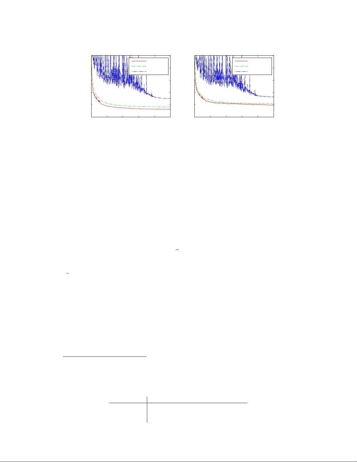
Pushing Stochastic Gradient towards Second-Order Methods – Backpr opagation Lear ning with T ransf ormations in Nonlinearities T ommi V atanen, T apani Raiko, Harri V alpola Department of Information and Computer Science Aalto Univ ersity School of Science P .O.Box 15400, FI-00076, Aalto, Espoo, Finland first.last@aalto.fi Y ann LeCun New Y ork Uni versity 715 Broadway , New Y ork, NY 10003, USA firstname@cs.nyu.edu Abstract Recently , we proposed to transform the outputs of each hidden neuron in a multi- layer perceptron network to have zero output and zero slope on av erage, and use separate shortcut connections to model the linear dependencies instead. W e con- tinue the work by firstly introducing a third transformation to normalize the scale of the outputs of each hidden neuron, and secondly by analyzing the connections to second order optimization methods. W e show that the transformations make a simple stochastic gradient behav e closer to second-order optimization methods and thus speed up learning. This is shown both in theory and with experiments. The experiments on the third transformation show that while it further increases the speed of learning, it can also hurt performance by con verging to a worse local optimum, where both the inputs and outputs of many hidden neurons are close to zero. 1 Introduction Learning deep neural networks has become a popular topic since the in vention of unsupervised pretraining [4]. Some later works have returned to traditional back-propagation learning in deep models and noticed that it can also provide impressi ve results [6] giv en either a sophisticated learning algorithm [9] or simply enough computational power [2]. In this work we study back-propagation learning in deep networks with up to fi ve hidden layers, continuing on our earlier results in [10]. In learning multi-layer perceptron (MLP) networks by back-propagation, there are known transfor - mations that speed up learning [8, 11, 12]. For instance, inputs are recommended to be centered to zero mean (or e ven whitened), and nonlinear functions are proposed to have a range from -1 to 1 rather than 0 to 1 [8]. Schraudolph [12, 11] proposed centering all factors in the gradient to have zero mean, and further adding linear shortcut connections that bypass the nonlinear layer . Gradient factor centering changes the gradient as if the nonlinear acti v ation functions had zero mean and zero slope on average. As such, it does not change the model itself. It is assumed that the discrepancy between the model and the gradient is not an issue, since the errors will be easily compensated by the linear shortcut connections in the proceeding updates. Gradient factor centering leads to a significant speed-up in learning. 1 In this paper , we transform the nonlinear acti vation functions in the hidden neurons such that they hav e on av erage 1) zero mean, 2) zero slope, and 3) unit variance. Our earlier results in [10] in- cluded the first two transformations and here we introduce the third one. cdsaasd W e explain the usefulness of these transformations by studying the Fisher information matrix and the Hessian, e.g. by measuring the angle between the traditional gradient and a second order update direction with and without the transformations. It is well known that second-order optimization methods such as the natural gradient [1] or Ne w- ton’ s method decrease the number of required iterations compared to the basic gradient descent, but the y cannot be easily used with high-dimensional models due to heavy computations with large matrices. In practice, it is possible to use a diagonal or block-diagonal approximation [7] of the Fisher information matrix or the Hessian. Gradient descent can be seen as an approximation of the second-order methods, where the matrix is approximated by a scalar constant times a unit matrix. Our transformations aim at making the Fisher information matrix as close to such matrix as possible, thus diminishing the dif ference between first and second order methods. Matlab code for replicating the experiments in this paper is a v ailable at https://github.com/tvatanen/ltmlp- neuralnet 2 Proposed T ransformations Let us study a MLP-network with a single hidden layer and shortcut mapping, that is, the output column vectors y t for each sample t are modeled as a function of the input column vectors x t with y t = Af ( Bx t ) + Cx t +  t , (1) where f is a nonlinearity (such as tanh ) applied to each component of the argument vector sepa- rately , A , B , and C are the weight matrices, and  t is the noise which is assumed to be zero mean and Gaussian, that is, p (  it ) = N   it ; 0 , σ 2 i  . In order to a void separate bias vectors that complicate formulas, the input vectors are assumed to have been supplemented with an additional component that is always one. Let us supplement the tanh nonlinearity with auxiliary scalar v ariables α i , β i , and γ i for each nonlinearity f i . They are updated before each gradient ev aluation in order to help learning of the other parameters A , B , and C . W e define f i ( b i x t ) = γ i [tanh( b i x t ) + α i b i x t + β i ] , (2) where b i is the i th row v ector of matrix B . W e will ensure that T X t =1 f i ( b i x t ) = 0 (3) T X t =1 f 0 i ( b i x t ) = 0 (4) " T X t =1 f i ( b i x t ) 2 T # " T X t =1 f 0 i ( b i x t ) 2 T # = 1 (5) by setting α i , β i , and γ i to α i = − 1 T T X t =1 tanh 0 ( b i x t ) (6) β i = − 1 T T X t =1 [tanh( b i x t ) + α i b i x t ] (7) γ i = n 1 T T X t =1 [tanh( b i x t ) + α i b i x t + β i ] 2 o 1 / 4 n 1 T T X t =1  tanh 0 ( b i x t ) + α i  2 o 1 / 4 . (8) 2 One way to motiv ate the first two transformations in Equations (3) and (4), is to study the expected output y t and its dependency of the input x t : 1 T X t y t = A 1 T X t f ( Bx t ) + C 1 T X t x t (9) 1 T X t ∂ y t ∂ x t = A " 1 T X t f 0 ( Bx t ) # B T + C . (10) W e note that by making nonlinear acti vations f ( · ) zero mean in Eq. (3), we disallow the nonlinear mapping Af ( B · ) to af fect the expected output y t , that is, to compete with the bias term. Similarly , by making the nonlinear activ ations f ( · ) zero slope in Eq. (4), we disallo w the nonlinear mapping Af ( B · ) to af fect the expected dependency of the input, that is, to compete with the linear mapping C . In traditional neural networks, the linear dependencies (e xpected ∂ y t /∂ x t ) are modeled by many competing paths from an input to an output (e.g. via each hidden unit), whereas our architecture gathers the linear dependencies to be modeled only by C . W e argue that less competition between parts of the model will speed up learning. Another e xplanation for choosing these transformations is that the y make the nondiagonal parts of the Fisher information matrix closer to zero (see Section 3). The goal of Equation (5) is to normalize both the output signals (similarly as data is often normalized as a preprocessing step – see,e.g., [8]) and the slopes of the output signals of each hidden unit at the same time. This is moti vated by observing that the diagonal of the Fisher information matrix contains elements with both the signals and their slopes. By these normalizations, we aim pushing these diagonal elements more similar to each other . As we cannot normalize both the signals and the slopes to unity at the same time, we normalize their geometric mean to unity . The ef fect of the first two transformations can be compensated exactly by updating the shortcut mapping C by C new = C old − A ( α new − α old ) B − A ( β new − β old ) [0 0 . . . 1] , (11) where α is a matrix with elements α i on the diagonal and one empty row below for the bias term, and β is a column vector with components β i and one zero belo w for the bias term. The third transformation can be compensated by A new = A old γ old γ − 1 new , (12) where γ is a diagonal matrix with γ i as the diagonal elements. Schraudolph [12, 11] proposed centering the factors of the gradient to zero mean. It was argued that deviations from the gradient fall into the linear subspace that the shortcut connections operate in, so they do not harm the ov erall performance. T ransforming the nonlinearities as proposed in this paper has a similar effect on the gradient. Equation (3) corresponds to Schraudolph’ s activity centering and Equation (4) corresponds to slope centering . 3 Theoretical Comparison to a Second-Order Method Second-order optimization methods, such as the natural gradient [1] or Newton’ s method, decrease the number of required iterations compared to the basic gradient descent, but they cannot be easily used with lar ge models due to heavy computations with large matrices. The natural gradient is the basic gradient multiplied from the left by the in verse of the Fisher information matrix. Using basic gradient descent can thus be seen as using the natural gradient while approximating the Fisher information with a unit matrix multiplied by the in verse learning rate. W e will show how the first two proposed transformations move the non-diagonal elements of the Fisher information matrix closer to zero, and the third transformation mak es the diagonal elements more similar in scale, thus making the basic gradient behav e closer to the natural gradient. The Fisher information matrix contains elements G ij = X t  ∂ 2 log p ( y t | x t , A , B , C ) ∂ θ i ∂ θ j  , (13) 3 where h·i is the expectation over the Gaussian distribution of noise  t in Equation (1), and vector θ contains all the elements of matrices A , B , and C . Note that here y t is a random variable and thus the Fisher information does not depend on the output data. The Hessian matrix is closely related to the Fisher information, but it does depend on the output data and contains more terms, and therefore we show the analysis on the simpler Fisher information matrix. The elements in the Fisher information matrix are: ∂ ∂ a ij ∂ ∂ a i 0 j 0 log p =  0 i 0 6 = i − 1 σ 2 i P t f j ( b j x t ) f j 0 ( b j 0 x t ) i 0 = i, (14) where a ij is the ij th element of matrix A , f j is the j th nonlinearity , and b j is the j th row vector of matrix B . Similarly ∂ ∂ b j k ∂ ∂ b j 0 k 0 log p = − X i 1 σ 2 i a ij a ij 0 X t f 0 j ( b j x t ) f 0 j 0 ( b j 0 x t ) x kt x k 0 t (15) and ∂ ∂ c ik ∂ ∂ c i 0 k 0 log p =  0 i 0 6 = i − 1 σ 2 i P t x kt x k 0 t i 0 = i. (16) The cross terms are ∂ ∂ a ij ∂ ∂ b j 0 k log p = − 1 σ 2 i a ij 0 X t f j ( b j x t ) f 0 j 0 ( b j 0 x t ) x kt (17) ∂ ∂ c ik ∂ ∂ a i 0 j log p =  0 i 0 6 = i − 1 σ 2 i P t f j ( b j x t ) x kt i 0 = i (18) ∂ ∂ c ik ∂ ∂ b j k 0 log p = − 1 σ 2 i a ij X t f 0 j ( b j x t ) x kt x k 0 t . (19) Now we can notice that Equations (14 – 19) contain factors such as f j ( · ) , f 0 j ( · ) , and x it . W e ar - gue that by making the factors as close to zero as possible, we help in making nondiagonal ele- ments of the Fisher information closer to zero. For instance, E [ f j ( · ) f j 0 ( · )] = E [ f j ( · )] E [ f j 0 ( · )] + Cov [ f j ( · ) , f j 0 ( · )] , so assuming that the hidden units j and j 0 are representing dif ferent things, that is, f j ( · ) and f j 0 ( · ) are uncorrelated, the nondiagonal element of the Fisher information in Equation (14) becomes exactly zero by using the transformations. When the units are not completely uncorrelated, the element in question will be only approximately zero. The same argument applies to all other elements in Equations (15 – 19), some of them also highlighting the benefit of making the input data x t zero-mean. Naturally , it is unrealistic to assume that inputs x t , nonlinear activ ations f ( · ) , and their slopes f 0 ( · ) are all uncorrelated, so the goodness of this approximation is empirically e v aluated in the next section. The diagonal elements of the Fisher can be found in Equations (14 – 16) when i = i 0 , j = j 0 , and k = k 0 . There we find f ( · ) 2 and f 0 ( · ) 2 that we aim to k eep similar in scale by using the third transformation in Equation (5). 4 Empirical Comparison to a Second-Order Method Here we inv estigate how linear transformations affect the gradient by comparing it to a second-order method, namely Newton’ s algorithm with a simple regularization to make the Hessian in vertible. W e compute an approximation of the Hessian matrix using finite difference method, in which case k -th ro w vector h k of the Hessian matrix H is giv en by h k = ∂ ( ∇ E ( θ )) ∂ θ k ≈ ∇ E ( θ + δ φ k ) − ∇ E ( θ − δ φ k ) 2 δ , (20) where φ k = (0 , 0 , . . . , 1 , . . . , 0) is a vector of zeros and 1 at the k -th position, and the error func- tion E ( θ ) = − P t log p ( y t | x t , θ ) . The resulting Hessian might still contain some very small or 4 500 1500 2500 −6 −4 −2 0 Eigenvalue order Log 10 eigenvalue LTMLP no−gamma regular (a) Eigenv alues 0.01 0.03 0.1 0.5 0 20 40 60 80 100 µ Angle / degrees LTMLP no−gamma regular (b) Angles Figure 1: Comparison of (a) distributions of the eigen v alues of Hessians ( 2600 × 2600 matrix) and (b) angles compared to the second-order update directions using L TMLP and regular MLP . In (a), the eigen values are distributed most e venly when using L TMLP . (b) shows that gradients of the transformed networks point to the directions closer to the second-order update. ev en negati ve eigenv alues which cause its in version to blow up. Therefore we do not use the Hes- sian directly , but include a regularization term similarly as in the Le venber g-Marquardt algorithm, resulting in a second-order update direction ∆ θ = ( H + µ I ) − 1 ∇ E ( θ ) , (21) where I denotes the unit matrix. Basically , Equation (21) combines the steepest descent and the second-order update rule in such a w ay , that when µ gets small, the update direction approaches the Newton’ s method and vice versa. Computing the Hessian is computationally demanding and therefore we hav e to limit the size of the network used in the experiment. W e study the MNIST handwritten digit classification problem where the dimensionality of the input data has been reduced to 30 using PCA with a random rotation [10]. W e use a network with two hidden layers with architecture 30–25–20–10. The network was trained using the standard gradient descent with weight decay regularization. Details of the training are giv en in the appendix. In what follows, networks with all three transformations ( LTMLP , linearly transformed multi-layer perceptron network), with two transformations ( no-gamma where all γ i are fixed to unity) and a network with no transformations ( r e gular , where we fix α i = 0 , β i = 0 , and γ i = 1 ) were compared. The Hessian matrix was approximated according to Equation (20) 10 times in regular intervals during the training of networks. All figures are shown using the approximation after 4000 epochs of training, which roughly corresponds to the midpoint of learning. Howe ver , the results were parallel to the reported ones all along the training. W e studied the eigenv alues of the Hessian matrix ( 2600 × 2600 ) and the angles between the methods compared and second-order update direction. The distribution of eigenv alues in Figure 1a for the networks with transformations are more e ven compared to the regular MLP . Furthermore, there are fewer negati ve eigen values, which are not shown in the plot, in the transformed networks. In Figure 1b, the angles between the gradient and the second-order update direction are compared as a function of µ in Equation (21). The plots are cut when H + µ I ceases to be positiv e definite as µ decreases. Curiously , the update directions are closer to the second-order method, when γ is left out, suggesting that γ s are not necessarily useful in this respect. Figure 2 shows histograms of the diagonal elements of the Hessian after 4000 epochs of training. All the distributions are bimodal, but the distributions are closer to unimodal when transformations are used (subfigures (a) and (b)) 1 . Furthermore, the variance of the diagonal elements in log-scale is smaller when using L TMLP , σ 2 a = 0 . 90 , compared to the other two, σ 2 b = 1 . 71 and σ 2 c = 1 . 43 . This suggests that when transformations are used, the second-order update rule in Equation (21) corrects different elements of the gradient vector more e venly compared to a regular back- propagation learning, implying that the gradient v ector is closer to the second-order update direction when using all the transformations. 1 It can be also argued whether (a) is more unimodal compared to (b). 5 10 −4 10 −2 0 50 100 150 200 (a) L TMLP 10 −4 10 −2 10 0 0 50 100 150 200 (b) no-gamma 10 −4 10 −2 0 50 100 150 200 250 1−2 1−3 2−3 1−4 2−4 3−4 (c) regular Figure 2: Comparison of distributions of the diagonal elements of Hessians. Coloring according to legend in (c) shows which layers to corresponding weights connect (1 = input, 4 = output). Diagonal elements are most concentrated in L TMLP and most spread in the re gular MLP netw ork. Notice the logarithmic x-axis. T o conclude this section, there is no clear e vidence in way or another whether the addition of γ ben- efits the back-propagation learning with only α and β . Howe ver , there are some differences between these two approaches. In any case, it seems clear that transforming the nonlinearities benefits the learning compared to the standard back-propagation learning. 5 Experiments: MNIST Classification W e use the proposed transformations for training MLP networks for MNIST classification task. Experiments are conducted without pretraining, weight-sharing, enhancements of the training set or any other known tricks to boost the performance. No weight decay is used and as only regularization we add Gaussian noise with σ = 0 . 3 to the training data. Networks with two and three hidden layers with architechtures 784–800–800–10 (solid lines) and 784–400–400–400–10 (dashed lines) are used. Details are giv en in the appendix. Figure 3 shows the results as number of errors in classifying the test set of 10 000 samples. The results of the regular back-propagation without transformations, sho wn in blue, are well in line with previously published result for this task. When networks with same architecture are trained using the proposed transformations, the results are improved significantly . Howe ver , adding γ in addition to pre viously proposed α and β does not seem to affect results on this data set. The best results, 112 errors, is obtained by the smaller architecture without γ and for the three-layer architecture with γ the result is 114 errors. The learning seems to con ver ge faster , especially in the three-layer case, with γ . The results are in line what was obtained in [10] where the networks were re gularized more thoroughly . These results sho w that it is possible to obtain results comparable to dropout networks (see [5]) using only minimal regularization. 6 Experiments: MNIST A utoencoder Previously , we have studied an auto-encoder network using two transformations, α and β , in [10]. Now we use the same auto-encoder architecture, 784–500–250–30–250–500–784. Adding the third transformation γ for training the auto-encoder poses problems. Many hidden neurons in decoding layers (i.e., 4th and 5th hidden layers) tend to be relati vely inacti ve in the beginning of training, which induces corresponding γ s to obtain very large values. In our experiments, auto-encoder with γ s ev entually div erge despite simple constraint we experimented with, such as γ i ≤ 100 . This be- havior is illustrated in Figure 4. The subfigure (a) sho ws the distrib ution of variances of outputs of all hidden neurons in MNIST classification network used in Section 5 given the MNIST training data. The corresponding distribution for hidden neurons in the decoder part of the auto-encoder is shown in the subfigure (b). The “dead neurons“ can be seen as a peak in the origin. The corresponding γ s, constrained γ i ≤ 100 , can be seen in the subfigure (c). W e hypothesize that this behavior is due to the fact, that in the beginning of the learning there is not much information reaching the bottleneck layer through the encoder part and thus there is nothing to learn for the decoding neurons. According to our tentative experiments, the problem described above may be overcome by disabling γ s in the 6 0 50 100 150 100 120 140 160 180 200 220 240 Epochs Number of errors LTMLP no−gamma regular Figure 3: The error rate on the MNIST test set for L TMLP training, L TMLP without γ and regular back-propagation. The solid lines show results for networks with two hidden layers of 800 neurons and the dashed lines for networks with three hidden layers of 400 neurons. 0 1 2 3 0 50 100 150 200 250 Variance (a) MNIST classification 0 0.5 1 1.5 2 0 50 100 150 200 Variance (b) MNIST auto-encoder 0 50 100 0 100 200 300 γ (c) MNIST auto-encoder Figure 4: Histograms of (a-b) v ariation of output of hidden neurons giv en the MNIST training data and (c) γ s of the decoder part (4th and 5th hidden layer) in the MNIST auto-encoder . (a) shows a healthy distributions of v ariances, whereas in (b), which includes only variances of the decoder part, there are many “dead neurons”. These neurons induce corresponding γ s, histogram of which is shown in (c), to blo w up which eventually lead to di vergence. decoder network (i.e., fix γ = 1 ). Howe ver , this does not seem to speed up the learning compared to our earlier results with only two transformations in [10]. It is also be possible to experiment with weight-sharing or other constraints to ov ercome the difficulties with γ s. 7 Discussion and Conclusions W e hav e shown that introducing linear transformation in nonlinearities significantly improves the back-propagation learning in (deep) MLP networks. In addition to two transformation proposed earlier in [10], we propose adding a third transformation in order to push the Fisher information matrix closer to unit matrix (apart from its scale). The hypothesis proposed in [10], that the transfor - mations actually mimic a second-order update rule, was confirmed by experiments comparing the networks with transformations and regular MLP network to a second-order update method. How- ev er, in order to find out whether the third transformation, γ , we proposed in this paper, is really useful, more experiments ought to be conducted. It might be useful to design experiments where con vergence is usually very slo w , thus rev ealing possible dif ferences between the methods. As hy- perparameter selection and regularization are usually nuisance in practical use of neural networks, it would be interesting to see whether combining dropouts [5] and our transformations can provide a robust frame work enabling training of robust neural networks in reasonable time. 7 The effect of the first two transformations is very similar to gradient factor centering [12, 11], but transforming the model instead of the gradient makes it easier to generalize to other contexts: When learning by by MCMC, variational Bayes, or by genetic algorithms, one would not compute the basic gradient at all. For instance, consider using the Metropolis algorithm on the weight matrices, and expecially matrices A and B . W ithout transformations, the proposed jumps would affect the expected output y t and the expected linear dependency ∂ y t /∂ x t in Eqs. (9)–(10), thus often leading to lo w acceptance probability and poor mixing. With the proposed transformations included, longer proposed jumps in A and B could be accepted, thus mixing the nonlinear part of the mapping f aster . For further discussion, see [10], Section 6. The implications of the proposed transformations in these other contexts are left as future work. References [1] S. Amari. Natural gradient works ef ficiently in learning. Neural Computation , 10(2):251–276, 1998. [2] D. C. Ciresan, U. Meier , L. M. Gambardella, and J. Schmidhuber . Deep big simple neural nets excel on handwritten digit recognition. CoRR , abs/1003.0358, 2010. [3] X. Glorot and Y . Bengio. Understanding the dif ficulty of training deep feedforward neural networks. In Pr oceedings of the Thirteenth International Confer ence on Artificial Intelligence and Statistics (AIST ATS) , pages 249–256, 2010. [4] G. E. Hinton and R. R. Salakhutdinov . Reducing the dimensionality of data with neural net- works. Science , 313(5786):504–507, 2006. [5] Geoffre y E. Hinton, Nitish Sriv astav a, Alex Krizhevsk y , Ilya Sutskev er , and Ruslan Salakhut- dinov . Improving neural networks by prev enting co-adaptation of feature detectors. CoRR , abs/1207.0580, 2012. [6] A. Krizhe vsky , I. Sutskev er , and G. E. Hinton. Imagenet classification with deep con volutional neural networks. 2012. [7] N. Le Roux, P . A. Manzagol, and Y . Bengio. T opmoumoute online natural gradient algorithm. In Advances in Neural Information Pr ocessing Systems 20 (NIPS*2007) , 2008. [8] Y . LeCun, L. Bottou, G. B. Orr , and K.-R. M ¨ uller . Efficient backprop. In Neural Networks: tricks of the tr ade . Springer-V erlag, 1998. [9] J. Martens. Deep learning via Hessian-free optimization. In Pr oceedings of the 27th Interna- tional Confer ence on Machine Learning (ICML) , 2010. [10] T apani Raiko, Harri V alpola, and Y ann LeCun. Deep learning made easier by linear transfor- mations in perceptrons. Journal of Machine Learning Researc h - Pr oceedings T rack , 22:924– 932, 2012. [11] N. N. Schraudolph. Accelerated gradient descent by factor-centering decomposition. T echnical Report IDSIA-33-98, Istituto Dalle Molle di Studi sull’Intelligenza Artificiale, 1998. [12] N. N. Schraudolph. Centering neural network gradient factors. In Genevie ve Orr and Klaus- Robert Mller , editors, Neural Networks: T ricks of the T rade , v olume 1524 of Lectur e Notes in Computer Science , pages 548–548. Springer Berlin / Heidelberg, 1998. A ppendix Details of Section 4 In experiments of Section 4, networks with all three transformations (L TMLP), only α and β (no- gamma) and network with no transformations (regular) were compared. Full batch training without momentum was used to make things as simple as possible. The networks were regularized using weight decay and adding Gaussian noise to the training data. Three hyperparameters, weight de- cay term, input noise variance and learning rate, were validated for all networks separately . The input data was normalized to zero mean and the network was initialized as proposed in [3], that is, the weights were drawn from a uniform distribution between ± √ 6 / √ n j + n j +1 , where n j is the number of neurons on the j th layer . 8 20 40 60 80 100 0 2 4 6 8 10 Training error / % Training time / % LTMLP no−gamma regular (a) Training error 20 40 60 80 100 0 2 4 6 8 10 Test error / % Training time / % LTMLP no−gamma regular (b) T est error Figure 5: Comparison of (a) training and (b) test errors of the algorithms using the MNIST data in the experiment comparing them to the second-order method. Note how the best learning for the regular MLP is relati vely high, leading to oscillations until it is annealed towards the end. W e sampled the three hyperparameters randomly (giv en our best guess intervals) for 500 runs and selected the median of the runs that resulted in the best 50 v alidation errors as the hyperparameters. Resulting hyperparameters are listed in T able 1. Notable differences occur in step sizes, as it seems that networks with transformations allo w using significantly larger step size which in turn results in more complete search in the weight space. Our weight updates are giv en by θ τ = θ τ − 1 − ε τ ∇ θ τ . (22) where the learning rate on iteration τ , ε τ , is giv en by ε τ =  ε 0 τ ≤ T / 2 2(1 − τ T ) ε 0 τ > T / 2 (23) that is, the learning rate starts decreasing linearly after the midpoint of the gi ven training time T . Furthermore, the learning rate ε τ is dampened for shortcut connection weights by multiplying with  1 2  s , where s is number of skipped layers as proposed in [10]. 2 Figure 5 sho ws training and test errors for the networks. The L TMLP obtains the best results although there is no big difference compared to training without γ . Details of Section 5 The MNIST dataset consists of 28 × 28 images of hand-drawn digits. There are 60 000 training samples and 10 000 test samples. W e experimented with two networks with two and three hidden layers and number of hidden neurons by arbitrary choice. Training was done in minibatch mode with 1000 samples in each batch and transformations are updated on every iteration using the current minibatch with using (6)–(8). This seems to speed up learning compared to the approach in [10] where transformations were updated only occasionally with the full training data. Random Gaussian noise with σ = 0 . 3 w as injected to the training data in the beginning of each epoch. 2 This heuristic is not well supported by analysis of Figure 2 and could be re-examined. T able 1: Hyperparameters for the neural networks L TMLP no-gamma regular weight decay 4 . 6 × 10 − 5 1 . 3 × 10 − 5 3 . 9 × 10 − 5 noise 0.31 0.36 0.29 step size 1.2 2.5 0.45 9 Our weight update equations are giv en by: ∆ θ τ = ∇ θ + p τ ∆ θ t − 1 , (24) θ τ = θ τ − 1 − ε τ ∆ θ τ , (25) where ε τ =  ε 0 τ ≤ T ε 0 f τ − T τ > T (26) p τ =  τ T p f + (1 − τ T ) p 0 τ ≤ T p f τ > T (27) In the equations abov e, T is a “burn-in time” where momentum p τ is increased from starting value p 0 = 0 . 5 to p f = 0 . 9 and learning rate ε = ε 0 is kept constant. When τ > T momentum is kept constant and learning rate starts decreasing exponentially with f = 0 . 9 . Hyperparameters were not validated but chosen by arbitrary guess such that learning did not diver ge. For the regular training, ε 0 = 0 . 05 w as selected since it div erged with higher learning rates. Then according to lessons learned, e.g. in Section 4, ε 0 = 0 . 3 was set for L TMLP with γ and ε 0 = 0 . 7 for the variant with no γ . Basically , it seems that transformations allow using higher learning rates and thus enable faster con vergence. 10