Higher order scrambled digital nets achieve the optimal rate of the root mean square error for smooth integrands

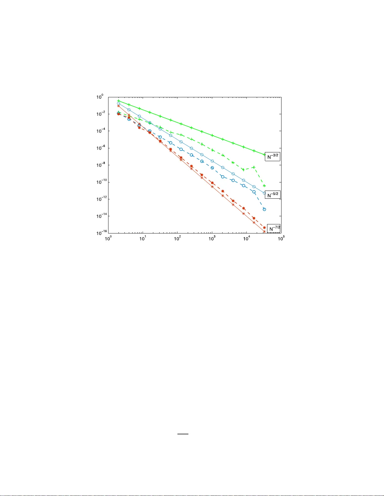
The Annals of Statistics 2011, V ol. 39, No. 3, 1372–13 98 DOI: 10.1214 /11-AOS880 c  Institute of Mathematical Statistics , 2 011 HIGHER ORDER SCRAMBLE D DIGIT AL NETS ACHIEVE THE OPTIMAL RA TE OF THE ROO T MEA N SQUARE ERR OR F OR SMOOTH INTEGRANDS By Josef Di ck 1 University o f New South W ales W e study a random sampling technique t o approximate integrals R [0 , 1] s f ( x ) d x by ave raging the fun ction at some sampling p oints. W e focus on cases where th e in tegrand is s mo oth, whic h is a p roblem whic h occurs in statistics. The conv ergence rate of th e approximation error depend s on the smoothn ess of the function f and th e sa mpling technique. F or in- stance, Mon te Carlo (MC) sampling yields a converg ence of the ro ot mean square error (RMSE) of o rder N − 1 / 2 (where N is the n um- b er of samples) for functions f with finite vari ance. Randomized QMC (R QMC), a com bination of MC and quasi-Monte Carlo ( QMC), ac hieves a RMSE of order N − 3 / 2+ ε under the stronger assumption that th e integrand h as b ounded v ariation. A combination of RQMC with lo cal an tithetic sampling achiev es a conve rgence of the RMS E of order N − 3 / 2 − 1 /s + ε (where s ≥ 1 is th e dimension) for functions with mixed partial deriv ativ es up to order t wo. Additional smoothn ess of the integrand does not improv e the rate of con vergence of these algorithms in general. On t he other hand, it is known that without additional smoothness of the integrand it is not p ossible t o improv e the con vergence rate. This pap er introd uces a new RQMC algorithm, for which w e prov e that it ac hieves a con vergence of the ro ot mean square error (RMSE) of order N − α − 1 / 2+ ε provided the integrand satisfies the strong as- sumption that it h as sq uare integrable partial mixed d eriva tives up to order α > 1 in each v ariable. Know n l ow er b ound s on t he RMSE sho w that th is rate of co nver gence cannot b e improv ed in general for integrands with this smo othness. W e provide numerical examples for which t h e R MSE conv erges approximatel y with order N − 5 / 2 and N − 7 / 2 , in accordance with t he th eoretical upp er b ound. Received July 2010; revised Jan uary 2011. 1 Supp orted by an Australian Researc h Council Queen Elizabeth II F ello wship. AMS 2000 subje ct classific ations. Primary 65C05; secondary 65D32. Key wor ds and phr ases. Digi tal nets, randomized quasi-Monte Carlo, quasi-Monte Carlo. This is an electro nic reprint of the or ig inal a rticle published by the Institute of Mathematica l Statistics in The A nnals of St atistics , 2011, V ol. 3 9, No. 3, 137 2–139 8 . This repr int differs from the or iginal in pagination and typogra phic detail. 1 2 J. DICK 1. In tro duction. In this pap er, w e introd u ce a rand om sampling tec h- nique to appro xim ate multiv ariate inte grals where the in tegrand is smo oth. Suc h problems app ear in stati stics, for instance in maxim u m lik elyho o d es- timations in v olving smo oth densit y fun ctions. W e consider the standardized problem of appro ximating the int egral ov er the unit cub e, R [0 , 1] s f ( x ) d x , that is, we assume that any tr an s formations necessary to c hange from different domains and densit y functions hav e al- ready b een carried out. The error of a pp ro ximating the integ ral dep en ds on the smo othness o f the in tegrand f and the samp ling te c hniqu e. It is kn o wn that the b est p ossible r ate of con ve rgence for an y alg orithm for the wo rst- case error is of order N − α + ε and for the ro ot mean square error is of order N − α − 1 / 2+ ε for f unctions w ith square in tegrable partial mixed deriv ativ es o f order α in eac h v ariable (here ε > 0 is used to hide p o we rs of log N fac- tors and can therefore be arbitrarily small a nd ev en 0 for the case α = 0 ). This means that imp ro v ed r ates of con v ergence can on ly b e ac hieved if the in tegrand satisfies ad d itional sm o othness assu mptions. O n the other hand, if an integrand has additional smo othn ess, not ev ery algorithm yields an impro ve d rate of con v ergence. In man y in s tances, algorithms which ac hiev e the b est p ossible rate of con v ergence for in tegrands with a giv en smo othness are kno w n . F or exam- ple, Mon te Carlo (M C) algorithms use i. i.d. uniform ly distr ibuted samples x 1 , . . . , x N ∈ [0 , 1] s to appro ximate the in tegral b y 1 N P N n =1 f ( x n ). F or func- tions f ∈ L 2 ([0 , 1] s ) the Mon te Carlo metho d has a ro ot mean squ are error (RMSE) of O ( N − 1 / 2 ). An alternativ e to Mon te Carlo is quasi-Mon te C arlo (QMC). In this metho d, one designs sample p oin ts w hic h are more u niformly distribution w ith r esp ect to some criterion (in one dimension this criterion is the Kolmogoro v–Smirnov distance b et w een t he u niform distribution and the sample p oin t distribution). These ac hieve a wo rst case error which d e- ca ys with O ( N − 1+ ε ) for an y ε > 0 for in tegrands w ith b oun ded v ariation; see [ 6 ]. O w en [ 14 – 16 ] in tro du ced a r andomization of QMC wh ic h ac hiev es a RMSE of O ( N − 3 / 2+ ε ), again for f unctions o f b ounded v ariation. Ow en’s randomization metho d uses a p ermutatio n app lied to digital nets (which is a construction sc heme f or sample points used in quasi-Mon te Carlo) c alled scram bling. Th ese algorithms ac hiev e the optimal r ate of con ve rgence for the class of functions menti oned ab ov e. A sligh t im p ro v ement of Ow en’s scrambling m etho d of digital nets can b e obtained b y com bining this appr oac h w ith local anti thetic sampling; see [ 18 ]. Th erein it w as shown that on e obtains a con vergence of the RMSE of O ( N − 3 / 2 − 1 /s + ε ) ( s is the dimension of the domain). The la tter metho d requires that the function f has contin u ous partial mixed deriv ativ es u p to order 2 in eac h coordin ate (note that the last metho d is not optimal for in tegrands with this smoothn ess). HIGHER OR DER SCRAMBLED DIGIT A L N ETS 3 Using the ab o v e m entioned algorithms, no further imp ro v emen t on the rate of conv ergence is obtained when one assumes that the in tegrand h as square integ rable partial mixed der iv ativ es of order α > 1 in eac h v ari- able. Th us, these algorithms are not optimal for in tegrands with additional smo othness. In this pap er , w e int ro d u ce a rand omization o f quasi-Mon te Carlo algo- rithms (wh ic h use d igital nets as quadrature p oin ts) su ch that the RMSE con v erges with O ( N − α − 1 / 2+ ε ) (for an y ε > 0) if the in tegrand has square in - tegrable partial mixed deriv ativ es up to order α in eac h v ariable. T his result holds for an y α > 0 and it is known that this resu lt is b est p ossib le; s ee [ 13 ]. Notice that it is necessary , in general and thus also for our algorithm, for the in tegrand to hav e additional smo othness to ac hiev e this rate of conv ergence. F or th e reader familiar with scram bled digital n ets, we br iefly describ e the algorithm. T he details on scram bled d igital nets will b e give n in the next section. 1.1. The algorithm. The underlyin g idea of the new randomized QMC algorithm s tems from [ 3 , 4 ]. Cen tral to this metho d is the digit inte rlacing function with in terlacing fac tor d ∈ N giv en by D d : [0 , 1) d → [0 , 1) , ( x 1 , . . . , x d ) 7→ ∞ X a =1 d X r =1 ξ r,a b − r − ( a − 1) d , where x r = ξ r, 1 b − 1 + ξ r, 2 b − 2 + · · · for 1 ≤ r ≤ d . W e also d efine this f unction for v ectors by setting D d : [0 , 1) ds → [0 , 1) s , ( x 1 , . . . , x ds ) 7→ ( D d ( x 1 , . . . , x d ) , . . . , D d ( x ( s − 1) d +1 , . . . , x sd )) . Let x 0 , . . . , x b m − 1 ∈ [0 , 1) ds b e a randomly scram bled digita l ( t, m, ds ) net o v er the fi nite field Z b of pr ime order b (we present the theoretical b ack- ground on scram bled digital n ets in the next s ection). Then one simply uses the sample points y n = D d ( x n ) ∈ [0 , 1) s for 0 ≤ n < b m . The in tegral is then esti mated using b I ( f ) = 1 b m b m − 1 X n =0 f ( y n ) . In Theorem 10 , w e sho w that if the in tegrand h as square in tegrable partial mixed deriv ativ es of order α ≥ 1 in eac h v ariable, then the v ariance of b I ( f ) satisfies V ar[ b I ( f )] = O ( N − 2 m in( d,α ) − 1+ ε ) for an y ε > 0, where N = b m is the n u m b er of s ample p oin ts. 4 J. DICK Fig. 1. The lines marke d by “ + ” show N − 3 / 2 and t he standar d deviation wher e d = 1 , the li nes marke d by “ ◦ ” show N − 5 / 2 and the standar d dev iation wher e d = 2 and the lines marke d by “ ∗ ” show N − 7 / 2 and the standar d deviation wher e d = 3 . Since s cr ambled digital nets (based on Sob ol p oints) are in clud ed in the statistics toolb o x of Ma tlab, this met ho d is v ery easy to implemen t (an im- plemen tation can b e found at http://q uasirando mideas.wordpress.com/ 2010/07/ 08/higher -order-scrambling ). 1.2. Numeric al r esults. Before w e in tro duce the theoretical bac kgroun d, w e present some simple numerical r esults whic h v erify the con v ergence re- sults. Example 1. In this example, the dimension is 1 and th e integrand is giv en by f ( x ) = x e x . Figure 1 sho ws the RMSE from 300 in dep endent replications. Here, th e straight lines sho w the fu nctions N − 3 / 2 , N − 5 / 2 and N − 7 / 2 . The other lines are the RMS E where the digit in terlacing f actor d is giv en by 1 for the up p er dashed line, 2 for the dashed line in the middle and 3 for the low est of the dashed lines. Figure 1 shows that in eac h case the RMSE conv erges appro ximately w ith ord er N − d − 1 / 2 (for large enough N ). (The result for d = 1 app ears to p erform ev en b etter than N − 3 / 2 .) Example 2. W e consider n ow a t w o-dimensional example where the in tegrand is giv en b y f ( x, y ) = y e xy e − 2 . This fun ction w as also u s ed in [ 18 ] HIGHER OR DER SCRAMBLED DIGIT A L N ETS 5 Fig. 2. The lines marke d by “ + ” show N − 3 / 2 and t he standar d deviation wher e d = 1 , the lines marke d by “ ◦ ” show N − 5 / 2 and the standar d deviation wher e d = 2 . where the sample p oints are obtained b y scrambling and lo cal an tithetic sampling. Figure 2 shows again the RMSE for 300 indep enden t replications. The straigh t lines sho w the functions N − 3 / 2 and N − 5 / 2 . Th e t w o dash ed lines sho w the RMSE when d = 1 (u p p er dashed lin e) and when d = 2 (lo w er dashed line). Figure 2 shows that in eac h case the RMSE con v erges appro x- imately with order N − d − 1 / 2 (for large enough N ). In the follo wing section, w e giv e the n ecessary b ac kgrou n d on QMC, dig- ital n ets, scram bling and W alsh fu nctions. W e then pro ve in Section 3 wh at can b e observ ed fr om the numerical results, n amely , that if the integrand has square in tegrable partial mixed deriv ativ es o f order α in eac h v ariable, then w e obtain a con v ergence of th e RMSE of O ( N − min ( α,d ) − 1 / 2+ ε ) for an y ε > 0. A sh ort d iscu ssion of the r esults is presente d in Section 4 . Some p rop erties of the digit in terlacing function D d necessary for the proof is present ed in Ap- p endix A and a technical pro of on th e co nv ergence of the W alsh coefficient s is presen ted in App endix B . 2. Bac kground and notation. In this section, w e giv e the n ecessary bac k- ground on QMC metho ds. Some n otatio n is required, which we n o w present. Here, c, C > 0 stand for generic constan ts whic h ma y d iffer in different places. Throughout the p ap er, w e assume that b ≥ 2 is a pr ime n umber. W e al- 6 J. DICK w a ys ha ve k = ( k 1 , . . . , k s ), k ′ = ( k ′ 1 , . . . , k ′ s ), x = ( x 1 , . . . , x s ), y = ( y 1 , . . . , y s ), x n = ( x n, 1 , . . . , x n,s ), y n = ( y n, 1 , . . . , y n,s ). 2.1. Quasi-Monte Carlo. QMC algorithms b I ( f ) = 1 N P N − 1 n =0 f ( x n ) are used to app ro ximate inte grals I ( f ) = R [0 , 1] s f ( x ) d x . Th e difference to Mon te Carlo is the method by which the sample p oin ts x 0 , . . . , x N − 1 ∈ [0 , 1) s are c hosen. The aim of QMC is to c h ose those points suc h that the in tegratio n error      Z [0 , 1] s f ( x ) d x − 1 N N − 1 X n =0 f ( x n )      ac hiev es the (almost) optimal rate of con v ergence as N → ∞ for a class of functions f : [0 , 1] s → R . F or instance, for the set of al l su c h functions f whic h h a v e b oun ded v ariation in the se nse of Hard y and Krause, whic h w e write as k f k HK < ∞ , it is kno wn that the b est rate of con v ergence for the w orst case error is e = sup f , k f k HK < ∞      Z [0 , 1] s f ( x ) d x − 1 N N − 1 X n =0 f ( x n )      ≍ N − 1+ ε for all ε > 0 . (More pr ecisely , there are constant s c, C > 0 such that cN − 1 (log N ) ( s − 1) / 2 ≤ e ≤ C N − 1 (log N ) s − 1 ; see [ 6 ].) Cho osing the p oints x 0 , . . . , x N − 1 ∈ [0 , 1) s i.i.d. uniformly d istributed as in MC d o es not yield this rate of con ve rgence. Even if a function h as b ound ed v ariation in th e sense of Hard y and Krause one obtains only a con v ergence of order N − 1 / 2 for i.i.d. uniformly distr ibuted sample p oin ts. There is an explicit construction of the sample p oin ts x 0 , . . . , x N − 1 for whic h the optimal rate of con v ergence is achiev ed. The essen tial insight is that the qu ad r ature p oints need to b e more uniformly distributed than what one obtains by c ho osing the samp le p oin ts by c hance. One criterion for how uniformly a set of p oints P N = { x 0 , . . . , x N − 1 } is distributed is t he star discrepancy D ∗ N ( P N ) = sup z ∈ [0 , 1] s      1 N N − 1 X n =0 1 x i ∈ [ 0 , z ) − V ol ([ 0 , z ))      , where [ 0 , z ) = Q s i =1 [0 , z i ) with z = ( z 1 , . . . , z s ), V ol([ 0 , z )) = Q s i =1 z i , the v ol- ume of [ 0 , z ) and 1 x i ∈ [ 0 , z ) =  1 , if x i ∈ [ 0 , z ), 0 , otherwise. When s = 1 , this b ecomes the Kolmogoro v–Sm irno v distance b etw een th e empirical distrib ution of the p oin ts and the unif orm distrib u tion. F urther, HIGHER OR DER SCRAMBLED DIGIT A L N ETS 7 w e call δ P N ( z ) = 1 N N − 1 X n =0 1 x i ∈ [ 0 , z ) − V ol([ 0 , z )) the local d iscrepancy (of P N ). The connection of this criterion to th e in tegration error is giv en by the Koksma–Hla wk a in equ alit y      Z [0 , 1] s f ( x ) d x − 1 N N − 1 X n =0 f ( x n )      ≤ D ∗ N ( P N ) k f k HK . An explicit construction of p oin t sets P N = { x 0 , . . . , x N − 1 } ∈ [0 , 1) s for whic h D ∗ N ( P N ) ≤ C N − 1 (log N ) s − 1 is give n by the concept of digital nets, whic h w e introdu ce in the next s ubsection. Notice that for suc h a p oin t set, the Koksm a–Hla wk a inequalit y implies the optimal rate of conv ergence of the int egration error, since for a giv en in tegrand, the v ariation k f k HK do es not dep end on P N and N . 2.2. Digital nets. W e in tro du ce th e basic id eas of digital n ets in the fol- lo wing. A compr eh ensiv e introd u ction to digital nets can b e found in [ 6 , 12 ]. The aim is to co nstru ct a point set P N = { x 0 , . . . , x N − 1 } suc h that the star discrepancy satisfies D ∗ N ( P N ) ≤ C N − 1 (log N ) s − 1 . T o do so, w e discretize the problem b y c ho osing the p oint s et P N suc h that the lo cal discrepancy δ P N ( z ) = 0 for certain z ∈ [0 , 1] s (those z in turn are chosen suc h that the star discrepancy of P N is small, as we exp lain b elo w). It turns out that, when on e c ho oses a base b ≥ 2 and N = b m , then for ev ery natural num b er m there exist p oin t sets P b m = { x 0 , . . . , x b m − 1 } suc h that δ P b m ( z ) = 0 for all z = ( z 1 , . . . , z s ) of the form z i = a i b d i for 1 ≤ i ≤ s, where 0 < a i ≤ b d i is an integ er and d 1 + · · · + d s ≤ m − t with d 1 , . . . , d s ≥ 0. Crucially , the v alue of t can b e c hosen ind ep endently of m (but dep endent on s ). A p oin t set P N whic h satisfies this pr op ert y is called a ( t, m, s ) -net in base b . An equiv alen t description o f ( t, m, s ) -nets in b ase b is give n in the follo w ing definition. Definition 1. Let b ≥ 2 , m, s ≥ 1 and t ≥ 0 b e inte gers. A p oint set P b m = { x 0 , . . . , x b m − 1 } ⊂ [0 , 1) s is called a ( t, m, s )-net in base b , if for all nonnegativ e in tegers d 1 , . . . , d s with d 1 + · · · + d s = m − t , the element ary in terv al s Y i =1  a i b d i , a i + 1 b d i  con tains exactly b t p oint s of P b m for all intege rs 0 ≤ a i < b d i . 8 J. DICK It ca n b e sho w n that a ( t, m, s )-net in base b satisfies D ∗ N ( P N ) ≤ C m s − 1 b m − 1 ; see [ 6 , 12 ] for d etails. Explicit constructions of ( t, m, s )-n ets can b e obtained using th e digital construction scheme. Suc h p oint sets are then called d igital nets [or digit al ( t, m, s )-nets if the p oin t set is a ( t, m , s ) -n et]. T o describ e the digital construction scheme, let b b e a prime num b er and let Z b b e the finite fi eld of order b (a prime p o w er and the finite field F b could b e used as wel l). Let C 1 , . . . , C s ∈ Z dm × m b b e s matrices of size dm × m with elemen ts in Z b and d ∈ N . The i th co ordin ate x n,i of the n th p oint x n = ( x n, 1 , . . . , x n,s ) of the digita l net is obtained in the follo wing wa y . F or 0 ≤ n < b m let n = n 0 + n 1 b + · · · + n m − 1 b m − 1 b e the base b rep r esen tation of n . Let ~ n = ( n 0 , . . . , n m − 1 ) ⊤ ∈ Z m b denote the ve ctor of digits of n . Th en let ~ y n,i = C i ~ n. F or ~ y n,i = ( y n,i, 1 , . . . , y n,i,dm ) ⊤ ∈ Z dm b , w e set x n,i = y n,i, 1 b + · · · + y n,i,dm b dm . The co nstru ction describ ed here is sligh tly m ore general to the classical concept to suit our needs (the classical construction sc heme uses d = 1 ). In this framework, w e hav e that if { x 0 , . . . , x b m − 1 } is a d igital ( t, m, ds ) -n et, then { D d ( x 0 ) , . . . , D d ( x b m − 1 ) } is a digital ( t, m, s )-net; see [ 5 ], Prop osition 1. The searc h for ( t, m, s ) -nets has no w been redu ced to finding suitable matrices C 1 , . . . , C s . Explicit constructions of su c h m atrices are a v ailable; see [ 6 , 12 ]. 2.3. Walsh functions. T o an alyze the RMSE, w e us e the W alsh series expansions of the in tegrands . In this subsection, w e recall some basic prop- erties of W alsh functions used in this pap er. First, we giv e the definition for the one-dimensional case. Definition 2. Let b ≥ 2 b e an in teger a nd represent k ∈ N 0 in base b , k = κ a − 1 b a − 1 + · · · + κ 0 , with κ i ∈ { 0 , . . . , b − 1 } . F urth er let ω b = e 2 π i/b . Th en the k th W alsh function b w al k : [0 , 1) → { 1 , ω b , . . . , ω b − 1 b } in base b is giv en by b w al k ( x ) = ω x 1 κ 0 + ··· + x a κ a − 1 b for x ∈ [0 , 1) with base b representati on x = x 1 b − 1 + x 2 b − 2 + · · · (unique i n the sense that in finitely man y of the x i are differen t from b − 1 ). W e no w extend this definition to the m ulti-dimensional case. HIGHER OR DER SCRAMBLED DIGIT A L N ETS 9 Definition 3. F or dimension s ≥ 2, x = ( x 1 , . . . , x s ) ∈ [0 , 1) s and k = ( k 1 , . . . , k s ) ∈ N s 0 , w e defin e b w al k : [0 , 1) s → { 1 , ω b , . . . , ω b − 1 b } b y b w al k ( x ) = s Y j = 1 b w al k j ( x j ) . As can b e seen f rom the d efinition, W alsh functions are piecewise constan t. F or b = 2, they are also related to Haar functions. W e need some notation to introd uce some fur ther prop erties of W alsh functions. By ⊕ , w e denote the digit wise add ition mo du lo b , that is, for x, y ∈ [0 , 1) with base b expansions x = P ∞ i =1 x i b − i and y = P ∞ i =1 y i b − i , w e define x ⊕ y = ∞ X i =1 z i b − i , where z i ∈ { 0 , . . . , b − 1 } is give n b y z i ≡ x i + y i (mo d b ), and let ⊖ den ote the d igit wise subtraction mo d ulo b . In the same man n er, we also define a digit wise addition and digit wise subtraction for nonnegati ve int egers based on the b -adic expansion. F or v ectors in [0 , 1) s or N s 0 , the op erators ⊕ and ⊖ are carried out comp onen t wise. Thr oughout this pap er, we alwa ys us e base b for the operations ⊕ and ⊖ . F u rther w e call x ∈ [0 , 1) a b -adic rati onal if it can b e written in a finite b ase b expansion. In t he fol lo wing prop osition, w e summarize some basic p rop erties of W alsh functions. Pr opo s ition 4. 1. F or al l k , l ∈ N 0 and al l x, y ∈ [0 , 1) , with the r estriction that if x, y ar e not q -adic r ationals, then x ⊕ y is not al lowe d to b e a b - adic r ational, we have b w al k ( x ) · b w al l ( x ) = w al k ⊕ l ( x ) , b w al k ( x ) · b w al k ( y ) = b w al k ( x ⊕ y ) . 2. We have Z 1 0 b w al 0 ( x ) d x = 1 and Z 1 0 b w al k ( x ) d x = 0 if k > 0 . 3. F or al l k , l ∈ N s 0 , we ha ve the fol lowing ortho gonality pr op erties: Z [0 , 1) s b w al k ( x ) b w al l ( x ) d x =  1 , if k = l , 0 , otherwise. 4. F or an y f ∈ L 2 ([0 , 1) s ) an d any σ ∈ [0 , 1) s , we ha ve Z [0 , 1) s f ( x ⊕ σ ) d x = Z [0 , 1) s f ( x ) d x . 5. F or s ∈ N , the system { b w al k : k = ( k 1 , . . . , k s ) , k 1 , . . . , k s ≥ 0 } is a c om- plete orthonormal system in L 2 ([0 , 1] s ) . 10 J. DICK The pro ofs of 1–3 are straigh tforw ard, and for a pro of of the remaining items see [ 2 ] or [ 6 , 20 ] for more information. Let d ≥ 1 and k 1 , . . . , k d ∈ N 0 . Let k i = κ i, 0 + κ i, 1 b + · · · , where κ i,a ∈ { 0 , . . . , b − 1 } and κ i,a = 0 for a large enough. T o analyze the RMSE, it is con v enien t to define a d igit in terlacing fun ction E d for natural num b ers, that is, E d : N d → N , ( k 1 , . . . , k d ) 7→ ∞ X a =0 d X r =1 κ r,a b r − 1+ ad . W e also extend this function to v ectors E d : N ds → N s , ( k 1 , . . . , k ds ) 7→ ( E d ( k 1 , . . . , k d ) , . . . , E d ( k d ( s − 1)+1 , . . . , k ds )) . Then w e ha ve b w al E d ( k 1 ,...,k d ) ( D d ( x 1 , . . . , x d )) = d Y i =1 b w al k i ( x i ) . 2.4. Scr ambling. The scram bling algorithm whic h yields th e optimal rate of con verge nce of the RMSE uses the digit int erlacing function and the scram bling in tro d uced b y O wen [ 14 – 16 ], which we describ e in the follo wing. 2.4.1. Owen ’s scr ambling. O w en’s scram bling algorithm is easiest de- scrib ed for s ome generic p oint x ∈ [0 , 1) s , with x = ( x 1 , . . . , x s ) and x i = ξ i, 1 b − 1 + ξ i, 2 b − 2 + · · · . The scram bled p oint shall b e denoted by y ∈ [0 , 1) s , where y = ( y 1 , . . . , y s ) and y i = η i, 1 b − 1 + η i, 2 b − 2 + · · · . The p oint y is obtained b y app lying p ermuta tions to eac h digit of ea c h coordinate of x . The p ermu- tation applied to ξ i,l dep ends on ξ i,k for 1 ≤ k < l . Sp ecifically , η i, 1 = π i ( ξ i, 1 ), η i, 2 = π i,ξ i, 1 ( ξ i, 2 ), η i, 3 = π i,ξ i, 1 ,ξ i, 2 ( ξ i, 3 ), and in general η i,k = π i,ξ i, 1 ,...,ξ i,k − 1 ( ξ i,k ) , (2.1) where π i,ξ i, 1 ,...,ξ i,k − 1 is a r andom p erm utation of { 0 , . . . , b − 1 } . W e assu me that p erm utations with different indices are c hosen mutually ind ep endent from eac h o ther and that eac h p ermuta tion is c h osen with the same p roba- bilit y . T o describ e Ow en’s scram bling, for 1 ≤ i ≤ s let Π i = { π i,ξ i, 1 ,...ξ i,k − 1 : k ∈ N , ξ i, 1 , . . . , ξ i,k − 1 ∈ { 0 , . . . , b − 1 }} , where for k = 1 we set π i,ξ i, 1 ,...,ξ i,k − 1 = π i , b e a giv en set of p erm utations and let Π = (Π 1 , . . . , Π s ). Then, w hen applyin g Ow en’s s cr ambling u sing HIGHER OR DER SCRAMBLED DIGIT A L N ETS 11 these p erm utations to some p oint x ∈ [0 , 1) s , w e write y = Π ( x ), wher e y is the point obtained by applyin g Ow en’s scram bling to x using the set of p ermutati ons Π = (Π 1 , . . . , Π s ). F or x ∈ [0 , 1) we drop the sub script i and just write y = Π( x ). 2.4.2. Owen ’s scr ambling of or der d . T o analyze the RMSE it is also con v enien t to generalize Owe n’s scrambling to h igher order. W e n o w describ e what we mean b y Owen’s scram bling of order d ≥ 1 for a generic p oint x ∈ [0 , 1) s . The scrambled p oin t y ∈ [0 , 1) s is giv en by y = D d ( Π ( D − 1 d ( x ))) , that is, one applies the inv erse mapp in g D − 1 d (see Ap p endix A for more information on D d ) to the p oint x to obtain a p oin t z ∈ [0 , 1) ds , applies Ow en’s scram bling of S ection 2.4.1 to z to obtain a p oin t w = Π ( z ) ∈ [0 , 1) ds and then use the trans formation D d to obtain the p oint y = D d ( w ) ∈ [0 , 1) s . Assuming that the p erm utations a re all c hosen with equ al probab ility , then the p oin t y is uniform ly distributed in [0 , 1) s . Pr opo s ition 5. L et x ∈ [0 , 1) s and let Π b e a uniformly and i.i.d. set of p ermutations. Then D d ( Π ( D − 1 d ( x ))) is uniformly distribute d in [0 , 1) s , that is, for any L eb esgue me asur able set G ⊆ [0 , 1) s , the pr ob ability that D d ( Π ( D − 1 d ( x ))) , denote d b y Pr ob[ D d ( Π ( D − 1 d ( x )))] = λ s ( G ) , wher e λ s de- notes t he s -dimensional L eb esgue me asur e. This result follo ws along the same lines as the pro of of [ 14 ], Prop osition 2. 2.4.3. Owen ’s lemma of or der d . A k ey r esult on scrambled nets is Owen’s lemma (see [ 15 ]) whic h w e no w generalize to in clude the ca se of scram bling of order d . Let k ∈ N ha v e base b represen tation k = κ 0 + κ 1 b + · · · + κ a b a . F or 0 ≤ r < d let k r = κ r b r + κ r + d b r + d + · · · + κ a r b a r , where a r ≤ a is the largest intege r suc h that d divides a r − r . If a < r , w e set k r = 0. F or x = ξ 1 b − 1 + ξ 2 b − 2 + · · · a nd x ′ = ξ ′ 1 b − 1 + ξ ′ 2 b − 2 + · · · a nd f or 0 ≤ r < d let β r b e the largest inte ger suc h that ξ r = ξ ′ r , ξ r + d = ξ ′ r + d , . . . , ξ r + β r d = ξ ′ r + β r d and ξ r +( β r +1) d 6 = ξ ′ r +( β r +1) d . Lemma 6. L et y , y ′ ∈ [0 , 1) b e two p oints obtaine d by applying Owen ’s scr ambling algor ithm of or der d ≥ 1 to the p oints x, x ′ ∈ [0 , 1) . (i) If k 6 = k ′ , then E [ b w al k ( y ) b w al k ′ ( y ′ )] = 0 . (ii) If k = k ′ and ther e exists an 0 ≤ r < d such that k r ≥ b β r +1 , then E [ b w al k ( y ⊖ y ′ )] = 0 . 12 J. DICK (iii) If k = k ′ and k r < b β r +1 for 0 ≤ r < d , then E [ b w al k ( y ⊖ y ′ )] = (1 − b ) − v , wher e v = |{ 0 ≤ r < d : b β r ≤ k r < b β r +1 }| . The pr o of of this result f ollo ws immediately fr om [ 6 ], L emma 13.23. In the next section, we analyze th e v ariance of the estimator b I ( f ) = 1 b m P b m − 1 n =0 f ( y n ). 3. V ariance of the estimator. Let f ∈ L 2 ([0 , 1] s ) hav e the follo wing W alsh series expansion f ( x ) ∼ X k ∈ N s 0 b f ( k ) b w al k ( x ) =: S ( x , f ) . (3.1) Although w e do not necessarily ha v e equalit y in ( 3.1 ), t he completeness o f the W alsh fu n ction sy s tem { b w al k : k ∈ N s 0 } (see [ 6 ]) implies that we do ha ve V ar[ f ] = X k ∈ N s 0 | b f ( k ) | 2 = V ar [ S ( · , f )] . (3.2) W e estimate the in tegral R [0 , 1] s f ( x ) d x b y b I ( f ) = 1 b m b m − 1 X n =0 f ( y n ) , where y 0 , . . . , y b m − 1 ∈ [0 , 1) s is obtained b y applyin g a r andom Owen scram- bling of order d to the digi tal ( t, m, s ) -net P b m = { x 0 , . . . , x b m − 1 } [b elo w we shall assume that there is a digita l ( t, m, ds )-net { z 0 , . . . , z b m − 1 } suc h that x n = D d ( z n ) for 0 ≤ n < b m , b ut for no w the assumption th at P b m is a digital ( t, m, s )-net is sufficien t]. F rom Prop osition 5 , it foll o ws that E [ b I ( f )] = Z [0 , 1] s f ( x ) d x . Hence, in the follo wing, we consider the v ariance o f the estimator b I ( f ) de- noted b y V ar[ b I ( f )] = E [( b I ( f ) − E [ b I ( f )]) 2 ] . The follo wing n otation is needed for the lemma b elo w. Let d ≥ 1 and l = ( l 1 , . . . , l s ) ∈ N ds 0 , where l i = ( l ( i − 1) d +1 , . . . , l id ). Let B d, l ,s = { ( k 1 , . . . , k ds ) ∈ N ds 0 : ⌊ b l i − 1 ⌋ ≤ k i < b l i for 1 ≤ i ≤ ds } . W e set σ 2 d, l ,s ( f ) = X k ∈ B d, l ,s | b f ( E d ( k )) | 2 . HIGHER OR DER SCRAMBLED DIGIT A L N ETS 13 Consider s = 1 for a momen t. Let l ∈ N d 0 . Then Lemma 6 implies that for ( k 1 , . . . , k d ) , ( k ′ 1 , . . . , k ′ d ) ∈ B d, l , 1 w e ha v e E [ b w al ( k 1 ,...,k d ) ( Π ( D − 1 d ( x ))) b w al ( k 1 ,...,k d ) ( Π ( D − 1 d ( x ′ )))] (3.3) = E [ b w al ( k ′ 1 ,...,k ′ d ) ( Π ( D − 1 d ( x ))) b w al ( k ′ 1 ,...,k ′ d ) ( Π ( D − 1 d ( x ′ )))] . Hence, for s ≥ 1 and l ∈ N ds 0 , c ho ose an arb itrary k ∈ B d, l ,s , and set Γ d, l ( P b m ) = 1 b 2 m b m − 1 X n,n ′ =0 s Y i =1 E [ b w al ( k d ( i − 1)+1 ,...,k di ) ( Π ( D − 1 d ( x n,i ))) × b w al ( k d ( i − 1)+1 ,...,k di ) ( Π ( D − 1 d ( x n ′ ,i )))] . Equation ( 3.3 ) implies that this definition is indep enden t of the particu- lar c hoice of k ∈ B d, l ,s . W e call Γ d, l ( P b m ) the gain c o efficient ( of P b m ) ( of or der d ). Lemma 7. L et d ≥ 1 . L et f ∈ L 2 ([0 , 1] s ) an d b I ( f ) = 1 b m b m − 1 X n =0 f ( y n ) , wher e y 0 , . . . , y b m − 1 ∈ [0 , 1) s is obtaine d by applying a r andom Owen scr am- bling of or der d to th e digital net P b m = { x 0 , . . . , x b m − 1 } . Then V ar[ b I ( f )] = X l ∈ N ds 0 \{ 0 } σ 2 d, l ,s ( f )Γ d, l ( P b m ) . Pr oof . Using the linea rity of expectation and Lemma 6 , w e get V ar[ b I ( f )] = E " X k , k ′ ∈ N s 0 \{ 0 } b f ( k ) b f ( k ′ ) 1 b 2 m b m − 1 X n,n ′ =0 b w al k ( y n ) b w al k ′ ( y n ′ ) # = X k , k ′ ∈ N s 0 \{ 0 } b f ( k ) b f ( k ′ ) 1 b 2 m b m − 1 X n,n ′ =0 s Y i =1 E [ b w al k i ( y n,i ) b w al k ′ i ( y n ′ ,i )] = X k ∈ N s 0 \{ 0 } | b f ( k ) | 2 1 b 2 m b m − 1 X n,n ′ =0 s Y i =1 E [ b w al k i ( y n,i ) b w al k i ( y n ′ ,i )] = X l ∈ N ds 0 \{ 0 } X k ∈ B d, l ,s | b f ( E d ( k )) | 2 14 J. DICK × 1 b 2 m b m − 1 X n,n ′ =0 s Y i =1 E [ b w al ( k d ( i − 1)+1 ,...,k di ) ( Π ( D − 1 d ( x n,i )) ⊖ Π ( D − 1 d ( x n ′ ,i )))] = X l ∈ N ds 0 \{ 0 } σ 2 d, l ,s ( f )Γ d, l ( P b m ) . Hence, the result follo ws.  T o obtain a b ound on th e v ariance V ar[ b I ( f )] , we prov e b ounds on σ d, l ,s ( f ) and Γ d, l ( P b m ), whic h w e consider in the foll o wing tw o sub sections. 3.1. A b ound on the gain c o efficients of or der d . In this section, we prov e a b ound on Γ d, l ( P b m ), wh ere the p oin t set is a digital ( t, m, s ) -net as con- structed in [ 4 ]. Lemma 8. L et { z 0 , . . . , z b m − 1 } b e a digital ( t, m, ds ) - net over Z b . L et x n = D d ( z n ) for 0 ≤ n < b m . Then the gain c o efficients of or der d for the digital ne t P b m = { x 0 , . . . , x b m − 1 } sa tisfy Γ d, l ( P b m ) ≤    0 , if | l | 1 ≤ m − t , b | q |−| l | 1 , if m − t < | l | 1 ≤ m − t + | q | , b − m + t , if | l | 1 > m − t + | q | . Pr oof . Let k = ( k 1 , . . . , k ds ) and l = ( l q , 0 ) for some q ⊆ { 1 , . . . , s } . Then from the pro of of [ 6 ], Corollary 1 3.7 and [ 6 ], Lemma 13 .8, it follo ws that Γ d, l ( P b m ) = 1 b 2 m b m − 1 X n,n ′ =0 s Y i =1 E [ b w al ( k d ( i − 1)+1 ,...,k di ) ( Π ( D − 1 d ( x n,i ))) × b w al ( k ′ d ( i − 1)+1 ,...,k ′ di ) ( Π ( D − 1 d ( x n ′ ,i )))] = 1 b 2 m b m − 1 X n,n ′ =0 s Y i =1 E [ b w al k ( Π ( z n )) b w al k ( Π ( z n ′ ))] =    0 , if | l | 1 ≤ m − t , b | q |−| l | 1 , if m − t < | l | 1 ≤ m − t + | q | , b − m + t , if | l | 1 > m − t + | q | . Hence, the result follo ws.  3.2. Higher or der variation. In this subsection, w e s tate a b ound on σ d, l ,s ( f ). T h e rate of deca y of σ d, l ,s ( f ) d ep ends on th e smo othness of the function f . W e measure th e smo othness using a v ariation based on finite HIGHER OR DER SCRAMBLED DIGIT A L N ETS 15 differences, which we introd uce in the follo wing. S ince th e smo othness of the function f ma y b e unk n o wn, w e cannot assume that w e can c ho ose d to b e th e smo othn ess. Hence, in the follo wing w e use α to d enote the smo othness of the integrand f . 3.2.1. Finite differ enc es. W e use a sligh t v ariation fr om classical fin ite differences. Let f : [0 , 1] → R and let z 1 , z 2 , . . . ∈ ( − 1 , 1) b e a sequence of n umb ers. Th en w e define ∆ 0 ( x ) f = f ( x ) and for α ≥ 1 we set ∆ α ( x ; z 1 , . . . , z α ) f = ∆ α − 1 ( x + z α ; z 1 , . . . , z α − 1 ) f − ∆ α − 1 ( x ; z 1 , . . . , z α − 1 ) f . F or instance, w e ha v e ∆ 1 ( x ; z 1 ) f = f ( x + z 1 ) − f ( x ) , ∆ 2 ( x ; z 1 , z 2 ) f = f ( x + z 1 + z 2 ) − f ( x + z 2 ) − f ( x + z 1 ) + f ( x ) , and in ge neral ∆ α ( x ; z 1 , . . . , z α ) f = X v ⊆{ 1 ,.. .,α } ( − 1) | v | f  x + X i ∈ v z i  , where | v | denotes the n u m b er of elements in v . W e alw a ys assume that x + P i ∈ v z i ∈ [0 , 1] for all v ⊆ { 1 , . . . , α } . If f is α times con tinuously differentiable, then th e mean v alue theorem implies that ∆ α ( x ; z 1 , . . . , z α ) f = z α ∆ α − 1 ( ζ 1 ; z 1 , . . . , z α − 1 ) d f d x , where min( x, x + z α ) ≤ ζ 1 ≤ max ( x, x + z α ). By induction, it then follo ws that ∆ α ( x ; z 1 , . . . , z α ) f = z 1 · · · z α d α f d x α ( ζ α ) , where x + min v ⊆{ 1 ,.. .,α } X i ∈ v z i ≤ ζ α ≤ x + max v ⊆{ 1 ,.. .,α } X i ∈ v z i . W e generalize the difference op erator to functions f : [0 , 1] s → R . Let α > 0 b e a nonnegativ e in teger. Let ∆ i,α b e the one-dimensional difference op erator ∆ α applied to the i th co ordinate of f . F or α = ( α 1 , . . . , α s ) ∈ { 0 , . . . , α } s and 1 ≤ i ≤ s let z i, 1 , . . . , z i,α i ∈ ( − 1 , 1). Then w e define ∆ α ( x ; ( z 1 , 1 , . . . , z 1 ,α 1 ) , . . . , ( z s, 1 , . . . , z s,α s )) f = ∆ 1 ,α 1 ( x 1 ; z 1 , 1 , . . . , z 1 ,α 1 ) · · · ∆ s,α s ( x s ; z s, 1 , . . . , z s,α s ) f 16 J. DICK = X v 1 ⊆{ 1 ,...,α 1 } · · · X v s ⊆{ 1 ,...,α s } ( − 1) | v 1 | + ··· + | v s | × f  x 1 + X i 1 ∈ v 1 z 1 ,i 1 , . . . , x s + X i s ∈ v s z s,i s  . If f has con tin uous mixed partial deriv ativ es up to order α in eac h v ari- able, then, as for the one-dimensional case, w e ha v e ∆ α ( x , ( z 1 , 1 , . . . , z 1 ,α 1 ) , . . . , ( z s, 1 , . . . , z s,α s )) f (3.4) = s Y i =1 α i Y r i =1 z i,r i ∂ α 1 + ··· + α s f ∂ x α 1 1 · · · ∂ x α s s ( ζ 1 ,α 1 , . . . , ζ s,α s ) , where w e set Q α i r i =1 z i,r i = 1 for α i = 0 and where x i + min v ⊆{ 1 ,.. .,α i } X r ∈ v z i,r ≤ ζ i,α i ≤ x i + max v ⊆{ 1 ,.. .,α i } X r ∈ v z i,r for 1 ≤ i ≤ s . Again w e assu me that x i + P r ∈ v z i,r ∈ [0 , 1] for all v ⊆ { 1 , . . . , α i } , ζ i,α i ∈ [0 , 1] for all 0 ≤ α i ≤ α and 1 ≤ i ≤ s . 3.2.2. V ariation. Let f : [0 , 1] s → R and α > 0 b e a nonnegativ e in teger. Let J = Q αs i =1 [ a i b l i , a i +1 b l i ), with 0 ≤ a i < b l i and l i ∈ N for 1 ≤ i ≤ αs . Apart from a t most a counta ble n umb er of p oints, the set D α ( J ) is the prod uct of a union of in terv als. Let α = ( α 1 , . . . , α s ) ∈ { 1 , . . . , α } s . Then we defin e the generalized Vitali v ariation b y V ( s ) α ( f ) = sup P  X J ∈P V ol( D α ( J )) sup     ∆ α ( t ; z 1 , . . . , z s ) f Q s i =1 Q α i r =1 z i,r     2  1 / 2 , (3.5) where the first su prem um su p P is extended o v er all partitions of [0 , 1) αs in to sub cub es of the form J = Q αs i =1 [ a i b l i , a i +1 b l i ) with 0 ≤ a i < b l i and l i ∈ N for 1 ≤ i ≤ αs , and the second su prem um is tak en o v er all t ∈ D α ( J ) and z i = ( z i, 1 , . . . , z i,α i ) with z i,r = τ i,r b − α ( l i − 1) − r where τ i,r ∈ { 1 − b, . . . , b − 1 } \ { 0 } f or 1 ≤ r ≤ α i and 1 ≤ i ≤ s and su c h that all the p oin ts at whic h f is ev aluated in ∆ α ( t ; z 1 , . . . , z s ) are in D α ( Q αs i =1 [ b − l i +1 ⌊ a i /b ⌋ , b − l i +1 ( ⌊ a i /b ⌋ + 1)). In App end ix A it is sho wn that V ol( D α ( J )) = V ol( J ) , the vo lume (i.e., Leb esgue mea sur e) of J . Hence, if the partial deriv ativ e ∂ α 1 + ··· + α s f ∂ x α 1 1 ··· ∂ x α s s are con- tin uous for a giv en ( α 1 , . . . , α s ) ∈ { 1 , . . . , α } s , then it can b e sh o wn that ( 3.4 ) and the mean v alue theorem imply that the s u m ( 3.5 ) is a Riemann s um f or the in tegral V ( s ) α ( f ) =  Z [0 , 1] s     ∂ α 1 + ··· + α s f ∂ x α 1 1 · · · ∂ x α s s ( x )     2 d x  1 / 2 . HIGHER OR DER SCRAMBLED DIGIT A L N ETS 17 F or ∅ 6 = u ⊆ { 1 , . . . , s } , let | u | denote the num b er of elemen ts in the set u and let V ( | u | ) α u ( f u ; u ) b e th e generalized Vitali v ariation with co efficien t α u ∈ { 1 , . . . , α } | u | of the | u | -dimensional function f u ( x u ) = Z [0 , 1] s −| u | f ( x ) d x { 1 ,...,s }\ u . F or u = ∅ , w e ha v e f ∅ = R [0 , 1] s f ( x ) d x and we define V ( | ∅ | ) α ( f ∅ ; ∅ ) = | f ∅ | . Then V α ( f ) =  X u ⊆{ 1 ,...,s } X α ∈{ 1 ,...,α } | u | ( V ( | u | ) α ( f u ; u )) 2  1 / 2 is called the generalized Hardy an d Krause v ariation of f of order α . A f u nc- tion f for which V α ( f ) is fi nite is said to b e of b ounded v ariation (of order α ). If the p artial deriv ative s ∂ α 1 + ··· + α s f ∂ x α 1 1 ··· ∂ x α s s are cont inuous for all ( α 1 , . . . , α s ) ∈ { 0 , . . . , α } s , then v ariation co incides w ith the norm V α ( f ) =  X u ⊆{ 1 ,...,s } X α ∈{ 1 ,...,α } | u | Z [0 , 1] | u |     Z [0 , 1] s −| u | ∂ P i ∈ u α i f Q i ∈ u ∂ x α i i d x { 1 ,...,s }\ u     2 d x u  1 / 2 . 3.2.3. The de c ay of the Walsh c o efficients for functions of b ounde d vari- ation. The follo wing lemma giv es a b ound on σ d, l ,s ( f ) for f unctions f of b ound ed v ariation of order α . Lemma 9. L et α, d ∈ N . L et f : [0 , 1] s → R with V α ( f ) < ∞ . L et b ≥ 2 b e an inte ger. L et l = ( l 1 , . . . , l ds ) ∈ N ds 0 and let K = { i ∈ { 1 , . . . , ds } : l i > 0 } . L et K i = K ∩ { ( i − 1) d + 1 , . . . , id } and α i = m in( α, | K i | ) for 1 ≤ i ≤ s . L et γ ′ j = ( b − 1) b − j +( i − 1) d − ( l j − 1) d for j ∈ K i and 1 ≤ i ≤ s . L et γ i, 1 < γ i, 2 < · · · < γ i,α i for 1 ≤ i ≤ s b e suc h that { γ i, 1 , . . . , γ i,α i } = { γ j : j ∈ K i } , that is, { γ i,j : 1 ≤ j ≤ α i } is just a r e or dering of the elements of the set { γ j : j ∈ K i } . Set γ ( l ) = Q s i =1 Q α i j = 1 γ i,j . Then σ d, l ,s ( f ) ≤ 2 s max( d − α, 0) γ ( l ) V α ( f ) . The pro of of this result is te c hn ical and is therefore deferred to Ap- p endix B . 3.3. Conver genc e r ate. W e can no w use Lemmas 7 – 9 to pr o v e the main result of the paper . Theorem 10. L et α, d ∈ N . L e t f : [0 , 1] s → R satisfy V α ( f ) < ∞ . L et b I ( f ) = 1 b m b m − 1 X n =0 f ( y n ) , 18 J. DICK wher e y 0 , . . . , y b m − 1 ∈ [0 , 1) s with y n = D d ( Π ( x n )) and x 0 , . . . , x b m − 1 ∈ [0 , 1) ds is a digital ( t, m , ds ) - net and the p ermutations in Π ar e c hosen uniformly and i. i .d. Then V ar[ b I ( f )] ≤ C b,s,α V α ( f ) ( m − t ) min( α,d ) s + s b − (2 mi n( α,d )+1)( m − t ) , wher e C b,s,α > 0 is a c onstant which dep ends only on α, b, d, s , but not on m . Pr oof . Let d ≤ α . Then from Lemmas 7 – 9 and the fac t that V d ( f ) ≤ V α ( f ) we obtai n that V ar[ b I ( f )] ≤ V α ( f )( b − 1) 2 ds b s + d ( d − 1) b − ( m − t +1) X l ∈ N ds 0 , | l | 1 >m − t b − 2 d | l | 1 ≤ V α ( f )( b − 1) 2 ds b s + d ( d − 1) b − ( m − t +1) ∞ X k = m − t +1 b − 2 dk  k + ds − 1 ds − 1  ≤ V α ( f )( b − 1) 2 ds ( b 2 d − 1) − ds b 2 d 2 s + s + d ( d − 1) b − (2 d +1)( m − t +1) ×  m − t + ds ds − 1  where w e used [ 6 ], Lemma 13 .24. Since  m − t + ds ds − 1  = ( m − t + ds ) · · · ( m − t + 2) ( ds − 1) · · · 1 ≤ ( m − t + 2) ds − 1 w e obtain V ar[ b I ( f )] ≤ C α,b,d,s V α ( f ) b − (2 d +1)( m − t ) ( m − t + 2) ds − 1 for some co nstant C α,b,d,s > 0 whic h dep ends only on α, b, d, s . Let n o w d > α . In the follo wing we sum o v er all l = ( l 1 , . . . , l s ) ∈ N ds 0 , where l i = ( l ( i − 1) d +1 , . . . , l id ), and suc h that l 1 + · · · + l ds > m − t . Let l ′ ( i − 1) d +1 ≥ l ′ ( i − 1) d +2 ≥ · · · ≥ l ′ id b e su c h that { l ′ ( i − 1) d +1 , . . . , l ′ id } = { l ( i − 1) d +1 , . . . , l id } , that is, the l ′ i are just a r eordering of the element s l i . There are at m ost ( d !) s reorderings whic h yield the same l ′ 1 , . . . , l ′ s . Then w e hav e α i Y j = 1 γ i,j ≤ ( b − 1) α i b ( d − 1)+( d − 2) + ··· +( d − α i ) α i Y j = 1 b − dl ′ i ≤ ( b − 1) α b d ( d − 1) / 2 b − d P α i j =1 l ′ ( i − 1) d + j . Hence, w e ha ve V ar[ b I ( f )] ≤ V α ( f )4 s ( d − α ) ( b − 1) 2 α b s + d ( d − 1) ( d !) s b − ( m − t +1) (3.6) × X l ∈ N ds 0 , | l | 1 >m − t l ordered b − 2 d P s i =1 P α j =1 l ( i − 1) d + j , HIGHER OR DER SCRAMBLED DIGIT A L N ETS 19 where l = ( l 1 , . . . , l ds ) ordered means that l ( i − 1) d +1 ≥ · · · ≥ l id for 1 ≤ i ≤ s . Hence, w e ha v e m − t < l 1 + · · · + l ds ≤ d α s X i =1 α X j = 1 l ( i − 1) d + j . Let no w k i = l ( i − 1) d +1 + · · · + l ( i − 1) d + α . Th en k i ≥ αl ( i − 1) d + j for α < j ≤ d and k 1 + · · · + k s ≥ α ( m − t ) /d . He nce, X l ∈ N ds 0 , | l | 1 >m − t l ordered b − 2 d P s i =1 P α j =1 l ( i − 1) d + j ≤ X k 1 ,...,k s ∈ N 0 ,k 1 + ··· + k s >α ( m − t ) /d b − 2 d ( k 1 + ··· + k s ) × s Y i =1  k i + α − 1 α − 1   k i α + 1  s ( d − α ) ≤ X p 1 ,...,p s ∈ N 0 ,p 1 + ··· + p s >α ( m − t ) b − 2( p 1 + ··· + p s ) × s Y i =1  ⌈ p i /d ⌉ + α − 1 α − 1   p i αd  + 1  s ( d − α ) ≤ X p 1 ,...,p s ∈ N 0 ,p 1 + ··· + p s >α ( m − t ) b − 2( p 1 + ··· + p s )  p i d + 2  sd ≤ ∞ X p = α ( m − t )+1 b − 2 p  p + s − 1 s − 1   p d + 2  sd ≤ ∞ X p = α ( m − t )+1 b − 2 p ( p + 2) sd + s − 1 ≤ b − 2 α ( m − t ) ( α ( m − t ) + 2) sd + s ( s ( d + 1) − 1) × max(1 , ( s ( d + 1) − 1) s ( d +1) − 1 ( α ( m − t ) + 1) − ( s ( d +1) − 1) × (log b ) − ( s ( d +1) − 1) ) . Th us, the result follo ws fr om ( 3.6 ).  4. Discussion. In this pap er, we ha ve extended the results of [ 16 , 18 ], by in tro ducing an algorithm and pro vin g that this algorithm can tak e adv an- tage of the smo othn ess of the in tegrand α , wh ere α ∈ N can b e arbitrarily 20 J. DICK large. Th eorem 10 sho ws t he con vergence rate of the standard deviation of the estimator b I ( f ) of O ( N − min ( α,d ) − 1 / 2 (log N ) s min( α +1 ,d +1) / 2 ). Th e n umer- ical resu lts in Section 1.2 u sing some to y exa mples also exhibit this r ate of con v ergence. T he upp er b ound is b est p ossible (apart from the pow er of the log N factor), since there is also a lo wer boun d o n the standard deviati on; see [ 13 ]. The impr o v emen t in the rate of con vergence in [ 18 ] h as been obtained b y using v ariance r ed uction tec hniqu es. Conv ersely , one migh t now ask wh ether the methods dev elop ed here ca n b e used to obtain new v ariance reduction tec h niques. (Some similarities b et w een this approac h and antithet ic sam- pling can be found in [ 5 ].) This is an op en question for future resea rch. Since the classical scram bling b y Ow en [ 14 ] is computationally to expen- siv e, v ariations of this scrambling sc heme ha ve b een int ro du ced whic h can easily b e implement ed. Matou ˇ sek [ 10 , 11 ] describ es an alternativ e scram- bling which uses fewe r p erm utations and is therefore easier to imp lement; see also [ 8 , 21 ]. Another scram bling sc heme wh ic h can b e imp lemen ted is b y T ezuk a and F aure [ 19 ]. See also [ 9 , 17 , 18 ] for o v erviews of v arious scram- blings. The id ea is to reduce the n umber of p ermuta tions required suc h that Ow en’s lemma still holds. Since the pro of of Lemma 6 follo ws along the s ame lines as th e pr o of of O w en’s lemma, the s implified scramblings menti oned ab o v e also apply here. The only alternativ e algorithm whic h ac hieve s the same conv ergence rate of the RMSE as prov en here is based on usin g an appro ximation A ( f ) to the in tegrand f and then applying MC to A ( f ) − f . The integ ral is then appro ximated by b I ( A ( f ) − f ) + R [0 , 1] s A ( f )( x ) d x w here R [0 , 1] s A ( f )( x ) d x can b e calculat ed an alytically . See [ 1 , 7 ] for details. APPENDIX A: PROPER TIES OF THE DIGIT INTERLACING FUNCTION The digit in terlacing function has several prop er ties whic h w e in v estigate in the follo wing and which we us e b elo w . Lemma 11. L et d > 1 . Then the mapping D d : [0 , 1) ds → [0 , 1) s is inje c- tive but not surje ctive. Pr oof . It suffices to sho w the result for s = 1. First, note that the digit expansion o f D d ( x 1 , . . . , x d ) is nev er of the form c 1 b − 1 + · · · + c j b − j +1 + ( b − 1) b − j + ( b − 1) b − j − d + ( b − 1 b − j − 2 d + · · · , since this w ould imply that there is a x j 0 , 1 ≤ j 0 ≤ d , whic h is a b -adic rational. But in this case we use the finite d igit expansions o f x j 0 and hence no v ector ( x 1 , . . . , x d ) ge ts mapp ed to this real n u m b er. Th us D d is not surjectiv e. HIGHER OR DER SCRAMBLED DIGIT A L N ETS 21 T o sho w that D d is in jectiv e, let ( x 1 , . . . , x d ) 6 = ( y 1 , . . . , y d ) ∈ [0 , 1) d . Hence, there exists an 1 ≤ i ≤ d suc h that x i 6 = y i , and hence there is a k ≥ 1 suc h that x i,k 6 = y i,k , where x i = x i, 1 b − 1 + x i, 2 b − 2 + · · · and y i = y i, 1 b − 1 + y i, 2 b − 2 + · · · (a nd where w e use the finite e xpans ions for b -adic rational s). Th us, t he digit expansions of D d ( x 1 , . . . , x d ) and D d ( y 1 , . . . , y d ) differ at least at one digit and hence D d ( x 1 , . . . , x d ) 6 = D d ( y 1 , . . . , y d ).  (Notice that a coun table n umber of element s could b e excluded fr om the set [0 , 1) s suc h that D d b ecomes bijectiv e.) Lemma 12. L et d ≥ 1 and J = Q ds i =1 [ a i , b i ) ⊆ [0 , 1] ds with a i ≤ b i for 1 ≤ i ≤ ds . L et λ n denote the L eb esgue me asur e on R n . Then λ ds ( J ) = λ s ( D d ( J )) . Pr oof . The result is trivial for d = 1 . Let no w d > 1 and consider s = 1 . Let J = Q d i =1 [ a i b − ν i , ( a i + 1) b − ν i ), where 0 ≤ a i < b ν i is an integ er and a i b ν i = a i, 1 b + a i, 2 b 2 + · · · + a i,ν i b ν i for some in tegers ν i ≥ 0 . Let ν = ( ν 1 , . . . , ν α ), | ν | ∞ = max 1 ≤ i ≤ s ν i and | ν | 1 = ν 1 + · · · + ν s . Then λ d ( J ) = b −| ν | 1 . Consider no w D d ( J ). Let 0 ≤ c < b d | ν | ∞ and cb − d | ν | ∞ = c 1 b + c 2 b 2 + · · · + c d | ν | ∞ b d | ν | ∞ with c 1 , . . . , c d | ν | ∞ ∈ { 0 , . . . , b − 1 } . W e h a v e D d ( J ) = [  c b d | ν | ∞ , c + 1 b d | ν | ∞  , where the union is o v er all c with expansion as ab ov e and where c 1 , . . . , c d | ν | ∞ ∈ { 0 , . . . , b − 1 } with the restriction that a i,k = c ( k − 1) d + i for 1 ≤ k ≤ ν i and 1 ≤ i ≤ d . Hence, there are d | ν | ∞ − | ν | 1 digits c j free to choose. Therefore, λ 1 ( D d ( J )) = λ 1  c b d | ν | ∞ , c + 1 b d | ν | ∞  b d | ν | ∞ −| ν | 1 = b −| ν | 1 . Therefore, the result holds for interv als of the form J . It follo ws that the result holds for in terv als o f the form J = Q ds i =1 [ a i b − ν i , ( a i + 1) b − ν i ), since this in terv al is simply a p ro duct of the p reviously con- sidered in terv als. Let no w J = Q ds i =1 [ a i , b i ) ⊆ [0 , 1) ds , with a i < b i for 1 ≤ i ≤ ds , b e an ar- bitrary in terv al. Since this in terv al ca n b e wr itten as a disjoint union of the elemen tary in terv als used ab ov e, the result also holds for these int erv als. 22 J. DICK Let ∅ 6 = I ⊆ { 1 , . . . , ds } and a i = b i for i ∈ I . Then λ ds ( J ) = 0. On the other hand, define b ′ i =  a i + b − ν , for i ∈ I , b i , otherwise, where ν is large enough such that b ′ i < 1 for all 1 ≤ i ≤ ds . Set J ′ = Q ds i =1 [ a i , b ′ i ). Then 0 ≤ λ s ( D d ( J )) ≤ λ s ( D d ( J ′ )) = λ ds ( J ′ ) ≤ b − ν → 0 as ν → ∞ . Hence, λ s ( D d ( J )) = 0.  APPENDIX B: PROOF O F LEMMA 9 Assume first that d ≥ α . Let l = ( l 1 , . . . , l ds ) ∈ N ds 0 and let K = { i ∈ { 1 , . . . , ds } : l i > 0 } . Let K i = K ∩ { ( i − 1) d + 1 , . . . , ( i − 1) d + d } . First, assume th at K i 6 = ∅ for i = 1 , . . . , s . Let l − 1 K = (( l 1 − 1) + , . . . , ( l ds − 1) + ) ∈ N ds 0 , where ( x ) + = max( x, 0). Let A l = { a = ( a 1 , . . . , a ds ) ∈ N ds 0 : 0 ≤ a i < b l i for 1 ≤ i ≤ ds } and [ a b − l , ( a + 1 ) b − l ) := ds Y i =1 [ a i b − l i , ( a i + 1) b − l i ) . Let q = ( q 1 , . . . , q αs ), w here q i = ⌊ a i /b ⌋ . In the follo wing w e w rite [ q b − l + 1 , ( q + 1 ) b − l + 1 ) for Q αs i =1 [ b − l i +1 ⌊ a i /b ⌋ , b − l i +1 ( ⌊ a i /b ⌋ + 1)). F u rther let D d ([ a b − l , ( a + 1 ) b − l )) = { D d ( x ) ∈ [0 , 1) s : x ∈ [ a b − l , ( a + 1 ) b − l ) } . Let x ∈ D d ([ a b − l , ( a + 1 ) b − l )), then X k ∈ A l b f ( E d ( k )) b w al E d ( k ) ( x ) = Z [0 , 1] s f ( t ) X k ∈ A l b w al E d ( k ) ( x ⊖ t ) d t = b | l | 1 Z D d ([ a b − l , ( a + 1 ) b − l ]) f ( t ) d t . F or l ∈ N ds 0 and a ∈ A l let c l , a = Z D d ([ a b − l , ( a + 1 ) b − l ]) f ( t ) d t . F or x ∈ D d ([ a b − l , ( a + 1 ) b − l )) let g ( x ) := X u ⊆ K ( − 1) | u | X k ∈ A l − ( 1 u , 0 ) b f ( E d ( k )) b w al E d ( k ) ( x ) = X u ⊆ K ( − 1) | u | b | l − ( 1 u , 0 ) | 1 c l − ( 1 u , 0 ) , ( ⌊ a u /b ⌋ , a { 1 ,...,ds }\ u ) , HIGHER OR DER SCRAMBLED DIGIT A L N ETS 23 where ( ⌊ a u /b ⌋ , a { 1 ,...,ds }\ u ) is the v ector whose i th coordin ate is ⌊ a i /b ⌋ if i ∈ u and a i if i ∈ { 1 , . . . , ds } \ u . Using Planc herel’s iden tit y , w e obtain σ 2 d, l ,s, r ( f ) = X u ⊆ K ( − 1) | u | X k ∈ A l − ( 1 u , 0 ) | b f ( E d ( k )) | 2 = Z 1 0 | g ( x ) | 2 d x = X a ∈ A l b −| l | 1     X u ⊆ K ( − 1) | u | b | l − ( 1 u , 0 ) | 1 c l − ( 1 u , 0 ) , ( ⌊ a u /b ⌋ , a { 1 ,...,ds }\ u )     2 = b | l | 1 X a ∈ A l     X u ⊆ K ( − 1) | u | b −| u | c l − ( 1 u , 0 ) , ( ⌊ a u /b ⌋ , a { 1 ,...,ds }\ u )     2 . W e can simplify the inner sum f urther. Let e = b ⌊ a /b ⌋ , that is, the i th comp onen t of e is giv en b y e i = b ⌊ a i /b ⌋ . F u rther, let d = a − e , that is, the i th comp onent of d is giv en by d i = a i − e i . Then w e hav e X u ⊆ K ( − 1) | u | b −| u | c l − ( 1 u , 0 ) , ( ⌊ a u /b ⌋ , a { 1 ,...,ds }\ u ) = X u ⊆ K ( − 1) | u | b −| u | X k u ∈ A 1 u c l , e +( k u , d { 1 ,...,ds }\ u ) = X u ⊆ K ( − 1) | u | b −| u | b − ds + | u | X k ∈ A 1 c l , e +( k u , d { 1 ,...,ds }\ u ) = b − ds X k ∈ A 1 X u ⊆ K ( − 1) | u | c l , a +( k u − d u , 0 { 1 ,...,ds }\ u ) = b − ds X k ∈ A 1 Z E a , l X u ⊆ K ( − 1) | u | f ( t + D d ( b − l ( k u − d u , 0 { 1 ,...,ds }\ u ))) d t , where E a , l = D d ([ a b − l , ( a + 1 ) b − l )) and w here we extend the digit in terlacing function D d to negativ e v alues b y usin g digits in { 1 − b, . . . , 0 } in case a comp onen t is negativ e. T o shorten the notation, we set δ k ( t ) = X u ⊆ K ( − 1) | u | f ( t + D d ( b − l ( k u − d u , 0 { 1 ,...,αs }\ u ))) . Therefore, σ 2 d, l ,s ( f ) ≤ b | l | 1 − 2 ds X a ∈ A l X k ∈ A 1 Z D d ([ a b − l , ( a + 1 ) b − l )) | δ k ( t ) | d t × X k ′ ∈ A 1 Z D d ([ a b − l , ( a + 1 ) b − l )) | δ k ′ ( t ) | d t 24 J. DICK = b | l | 1 − 2 ds X k , k ′ ∈ A 1 X a ∈ A l Z D d ([ a b − l , ( a + 1 ) b − l )) | δ k ( t ) | d t × Z D d ([ a b − l , ( a + 1 ) b − l )) | δ k ′ ( t ) | d t . Using Cauc h y–Sc hw arz’ inequalit y , we ha ve Z D d ([ a b − l , ( a + 1 ) b − l ]) | δ k ( t ) | d t ≤  Z D d ([ a b − l , ( a + 1 ) b − l ]) 1 d t  1 / 2  Z D d ([ a b − l , ( a + 1 ) b − l ]) | δ k ( t ) | 2 d t  1 / 2 = b −| l | 1 / 2  Z D d ([ a b − l , ( a + 1 ) b − l ]) | δ k ( t ) | 2 d t  1 / 2 . Let B a , k = ( R D d ([ a b − l , ( a + 1 ) b − l ]) | δ k ( t ) | 2 d t ) 1 / 2 . Then w e hav e σ 2 d, l ,s ( f ) ≤ b − 2 ds X k , k ′ ∈ A 1 X a ∈ A l B a , k B a , k ′ ≤ max k , k ′ ∈ A 1 X a ∈ A l B a , k B a , k ′ = max k ∈ A 1 X a ∈ A l B 2 a , k , where the last inequalit y follo ws as the Cauc h y–Sc hw arz inequalit y is an equalit y for t wo v ectors whic h are li nearly dep enden t. Let k ∗ b e the v alue of k ∈ A 1 for whic h the sum P a ∈ A l B 2 a , k tak es on its maxim um . Hence , σ 2 d, l ,s ( f ) ≤ X a ∈ A l Z D d ([ a b − l , ( a + 1 ) b − l ]) | δ k ∗ ( t ) | 2 d t . The follo wing lemma relates the fu nction δ k to the d ivided differences in tro duced ab o ve . Lemma 13. L et l , a , e , q , K and K 1 , . . . , K s b e define d as ab ove. F or t ∈ D d ([ a b − l , ( a + 1 ) b − l )) w e have | δ k ∗ ( t ) | ≤ 2 s ( d − α ) sup | ∆ α ( t ′ ; z 1 , . . . , z s ) f | , wher e α = ( α 1 , . . . , α s ) with α i = min( | K i | , α ) , and the supr emum is taken over al l t ′ ∈ D d ([ a b − l , ( a + 1 ) b − l )) and z i = ( z i, 1 , . . . , z i,α i ) with z i,r i = τ i,r i b − d ( l i − 1) − r i wher e τ i,r i ∈ { 1 − b, . . . , b − 1 } \ { 0 } for 1 ≤ r i ≤ | K i | and 1 ≤ i ≤ s and such th at al l the p oints at which f is evaluate d in ∆ α ( t ′ ; z 1 , . . . , z s ) ar e in D α ([ q b − l + 1 K , ( q + 1 ) b − l + 1 K )) . F urthermor e, we may assume that | z i, 1 | < | z i, 2 | < · · · < | z i, | K i | | for 1 ≤ i ≤ s . HIGHER OR DER SCRAMBLED DIGIT A L N ETS 25 Pr oof . W e sh o w that δ k ∗ ( t ) can b e written as divided differences. Sin ce the divided difference op erators are applied to eac h co ordinate sep arately , it suffices to sh o w the result for s = 1. In this case, we h a v e δ k ∗ ( t ) = X u ⊆ K ( − 1) | u | f ( t + D d ( b − l ( k ∗ u − d u , 0 { 1 ,...,d }\ u ))) , where no w K = { i ∈ { 1 , . . . , d } : l i > 0 } . Let l = ( l 1 , . . . , l d ). Let t = t 1 b + t 2 b 2 + · · · , a = ( a 1 , . . . , a d ) and a j = a j,l j + a j,l j − 1 b + · · · + a j, 1 b l j − 1 . Then for t ∈ D d ([ a b − l , ( a + 1 ) b − l )) w e ha v e t j + ( l − 1) d = a j,l for 1 ≤ l ≤ l j and j ∈ K. F urther, we ha ve d j = a j,l j for j ∈ K . Let I = { j + ( l − 1) d : 1 ≤ l ≤ l j , j ∈ K } . Then for t ∈ D d ([ a b − l , ( a + 1 ) b − l )) and u ⊆ K w e ha v e t + D d ( b − l ( k u − d u , 0 )) = X j ∈ K l j − 1 X l =1 a j,l b j + ( l − 1) d + X j ∈ u k j j + ( l j − 1) d + X j ∈ K \ u a j,l j b j + ( l j − 1) d + X j ∈ N \ I t j b j . F or giv en t ∈ D d ([ a b − l , ( a + 1 ) b − l )) let τ u = t + D d ( b − l ( k ∗ u − d u , 0 { 1 ,...,d }\ u )) . Let k ∗ = ( k ∗ 1 , . . . , k ∗ d ) and z j = k ∗ j − a j,l j b j + ( l j − 1) d for j ∈ K. Notice th at if z j = 0, then δ k ∗ ( t ) = 0 and hence we can exclude this case. Then for v ⊂ u ⊆ K we h a v e τ u − τ v = X j ∈ u \ v z j . Therefore, δ k ∗ ( t ) = X u ⊆ K ( − 1) | u | f ( t + D d ( b − l ( k ∗ u − d u , 0 { 1 ,...,d }\ u ))) = X u ⊆ K ( − 1) | u | f ( τ u ) = X u ⊆ K ( − 1) | u | f ( τ ∅ + ( τ u − τ ∅ )) = X u ⊆ K ( − 1) | u | f  t + X j ∈ u z j  = ∆ | K | ( t ; z ′ ) f , where z ′ = ( z j ) j ∈ K . 26 J. DICK Notice that the ordering of the element s in z ′ do es not c hange the v alue of ∆ | K | ( t ; z ′ ). Hence, assume that the elemen ts in z ′ are ordered suc h that z ′ 1 > z ′ 2 > · · · > z ′ | K | . F or the case where | K | > α , w e obtain fr om the d efinition of the divided differences that ∆ | K | ( t ; z ′ ) = X u ⊆{| K | +1 ,. . . ,α } ( − 1) | u | ∆ α  t + X j ∈ u z ′ j ; ( z ′ 1 , . . . , z ′ α )  . By taking the tr iangular inequalit y and the supr emum ov er all t ′ in { t + P j ∈ u z ′ j : u ⊆ {| K | + 1 , . . . , α }} , we obtain ∆ | K | ( t ; z ′ ) ≤ 2 α −| K | sup t ′ | ∆ α ( t ′ ; ( z ′ 1 , . . . , z ′ α )) | . Consider no w the general case s ≥ 1 and K = { i ∈ { 1 , . . . , ds } : l i > 0 } . Let K i = K ∩ { ( i − 1) d + 1 , . . . , ( i − 1) d + d } and α ′ i = | K i | for 1 ≤ i ≤ s . Let α ′ = ( α ′ 1 , . . . , α ′ s ). Let z j = k ∗ j − a j,l j b j − ( i − 1) d +( l j − 1) d for j ∈ K i and 1 ≤ i ≤ s and z ′ i = ( z j ) j ∈ K i for 1 ≤ i ≤ s . Then we obtain δ k ∗ ( t ) = ∆ α ′ ( t ; z ′ 1 , . . . , z ′ s ) f . Define now α i = min ( α, α ′ i ) for 1 ≤ i ≤ s and α = ( α 1 , . . . , α s ). Notice that α ′ i ≤ d a nd therefore s X i =1 ( α ′ i − α i ) ≤ s ( d − α ) . Notice that ∆ α ′ i can b e expressed as a sum an alternating su m of 2 α ′ i − α i summands ∆ α i . By taking the triangular inequalit y , w e therefore obtain | δ k ∗ ( t ) | = | ∆ α ′ ( t ; z 1 , . . . , z s ) f | ≤ 2 s ( d − α ) sup | ∆ α ( t ′ ; z 1 , . . . , z s ) | , where the supremum is tak en o ve r a ll admissib le choice s of z 1 , . . . , z s and t ′ . Hence, σ 2 d, l ,s ( f ) ≤ 2 s ( d − α ) X a ∈ A l Z D d ([ a b − l , ( a + 1 ) b − l ]) sup | ∆ α ( t ′ ; z 1 , . . . , z s ) f | 2 d t , where the suprem um is o ve r t he same set as in Lemma 13 . Therefore, σ 2 d, l ,s ( f ) ≤ 2 s ( d − α ) X a ∈ A l V ol( D d ([ a b − l , ( a + 1 ) b − l ])) su p | ∆ α ( t ′ ; z 1 , . . . , z s ) f | 2 ≤ 2 s ( d − α ) X q ∈ A l − 1 K V ol( D d ([ q b − l + 1 K , ( q + 1 ) b − l + 1 K ])) × sup | ∆ α ( t ′ ; z 1 , . . . , z s ) f | 2 . HIGHER OR DER SCRAMBLED DIGIT A L N ETS 27 Let γ ′ j = ( b − 1) b − j +( i − 1) d − ( l j − 1) d for j ∈ K i and 1 ≤ i ≤ s . Let γ i, 1 < γ i, 2 < · · · < γ i,α i for 1 ≤ i ≤ s b e such that { γ i, 1 , . . . , γ i,α i } = { γ j : j ∈ K i } , that is, { γ i,j : 1 ≤ j ≤ α i } is just a reordering of the elemen ts of the set { γ j : j ∈ K i } . Set γ ( l ) = Q s i =1 Q α i j = 1 γ i,j . Then σ 2 α, l ,s ( f ) ≤ 2 s ( d − α ) γ 2 ( l ) × X e ∈ A l − 1 K V ol( D α ([ q b − l + 1 K , ( q + 1 ) b − l + 1 K ])) × sup | ∆ α ( t ; z 1 , . . . , z s ) f | 2 Q i ∈ K | z i | 2 ≤ 2 s ( d − α ) γ 2 ( l ) V 2 α ( f ) , where the s upremum is o ver all adm issible t and z 1 , . . . , z s as describ ed in the lemma. Consider no w the case where K i = ∅ for some 1 ≤ i ≤ s . Let R = { i ∈ { 1 , . . . , s } : K i = ∅ } . Then the result follo ws by r eplacing f with the f unction R [0 , 1] | R | f ( x ) d x R in the p ro of abov e. Let now d < α . Th en V d ( f ) ≤ V α ( f ), and h en ce th e result follo ws b y using the pro of ab o v e with d = α . This co mpletes the pr o of.  REFERENCES [1] B ahv alov, N. S. (1959). Approximate computation of m ultiple integrals. V estnik Moskov. Univ. Ser. Mat. Meh. Ast r. Fi z. Him. 1959 3–18. MR0115275 [2] Ch restenson, H. E. (1955). A class of generalized Walsh funct ions. Pacific J. Math. 5 17–31. MR0068659 [3] Di ck, J. (2007). Explicit constructions of qu asi-Mon te Carlo rules for the numerical integ ration of high-dimensional perio dic functions. SIAM J. N um er. A nal. 45 2141–21 76 ( electronic). MR2346374 [4] Di ck, J. (2008). W alsh spaces con taining smooth functions and quasi-Mon te Carlo rules of arbitrary high order. SIAM J. Numer. A nal. 46 1519–1553. MR2391005 [5] Di ck, J. (2009). On quasi-Monte Ca rlo rules achieving higher order con verg ence. In Monte Carlo and Quasi-Monte Carlo M etho ds 2008 ( P. L’Ecuyer and A. Owen , eds.) 73–96. Springer, Berlin. [6] Di ck, J. an d Pillichshammer, F. (2010). Digital Nets and Se quenc es: D iscr ep ancy The ory and Quasi-Monte Carlo Inte gr ation . Cambridge Univ. Press, Cam bridge. MR2683394 [7] He inrich, S. (19 94). Random approximation in n umerical analysis. In F unctional Ana lysis (Essen, 1991) ( K. D. B ierstedt, A. Pietsch, W. M . Ruess an d D. Vo gt, ed s. ). L e ctur e Notes in Pur e and Appl. M ath. 150 123–171 . Dekker, New Y ork. MR1241675 [8] Hi ckernell, F. J. ( 1996). The mean square discrepancy of randomized nets. ACM T r ans. Mo deling Comput. Si mul. 6 274–296. [9] L’Ecuye r, P. and Le mieux, C. (2002). Recent adv ances in randomized qu asi- Mon te Carlo meth ods. In Mo deling Unc ertainty ( M . Dror, P. L’Ecuyer and 28 J. DICK F. Szidar ovszki, eds. ). Internat. Ser. Op er. R es. Management Sci. 46 419–474. Kluw er, Boston, MA. MR1893290 [10] Ma tou ˇ sek, J. (1998). On the L 2 -discrepancy for anc hored b oxes. J. Compl exity 14 527–556 . MR1659004 [11] Ma tou ˇ sek, J. (1999). Ge ometric Discr ep ancy: An Il lustr ate d Guide . Algorithms and Combinatorics 18 . Springer, Berlin. MR1697825 [12] Niederreiter, H. (1992). R andom Numb er Gener ation and Quasi-Monte Carlo Metho ds . CBMS-NSF R e gional Confer enc e Series in Applie d Mat hematics 63 . SIAM, Ph iladelphia, P A. MR1172997 [13] No v ak, E. (1988). Deterministic and Sto chastic Err or Bounds in Numeric al A nalysis . L e ctur e Notes in Math. 1349 . Springer, Berlin. MR0971255 [14] O wen, A . B. (1995). Randomly p ermuted ( t, m, s )-n ets and ( t, s )-sequences. I n Monte Carlo and Quasi-Monte Carlo Metho ds i n Scientific Com puting (Las V e- gas, NV, 1994) ( H. Niederre iter and J.-S. Shiue , eds. ). L e ctur e Notes in Statist. 106 299–317 . Sp ringer, New Y ork. MR1445791 [15] O wen, A. B. (1997). Monte Ca rlo v ariance of scram bled net q uadrature. SIA M J. Numer. Anal. 34 1884–1910 . MR1472202 [16] O wen, A. B. (1997). S cram bled net v ariance for integral s of smo oth functions. Ann. Statist. 25 1541– 1562. MR1463564 [17] O wen, A . B. (2003). V ariance with al ternative scram blings of digital nets. A CM T r ans. Mo del. Comp. Simul. 13 363–378. [18] O wen, A . B . (2008). Lo cal antithetic sampling with scram bled nets. A nn. Statist. 36 2319–2343. MR2458189 [19] Tezuka, S. and F a ure, H. (200 3). I -binomial scram bling of digital nets and se- quences. J. Com pl exity 19 744–7 57. MR2040428 [20] W alsh, J. L. (1923). A closed set of normal orthogonal functions. A mer. J. Math. 45 5–24. MR1506485 [21] Yue, R.-X. and Hi ckernell, F. J. (2002). The discrepancy and gain co efficients of scram bled digital nets. J. Complexity 18 135–151 . MR1895080 School of Ma themat ics and St a tistics University of New South W a les Sydney NSW 20 52 Aust ralia E-mail: josef.dick@unsw.edu.au URL: htt p://profiles.unsw.edu.au/maths/jdick 1