Provably Safe and Robust Learning-Based Model Predictive Control

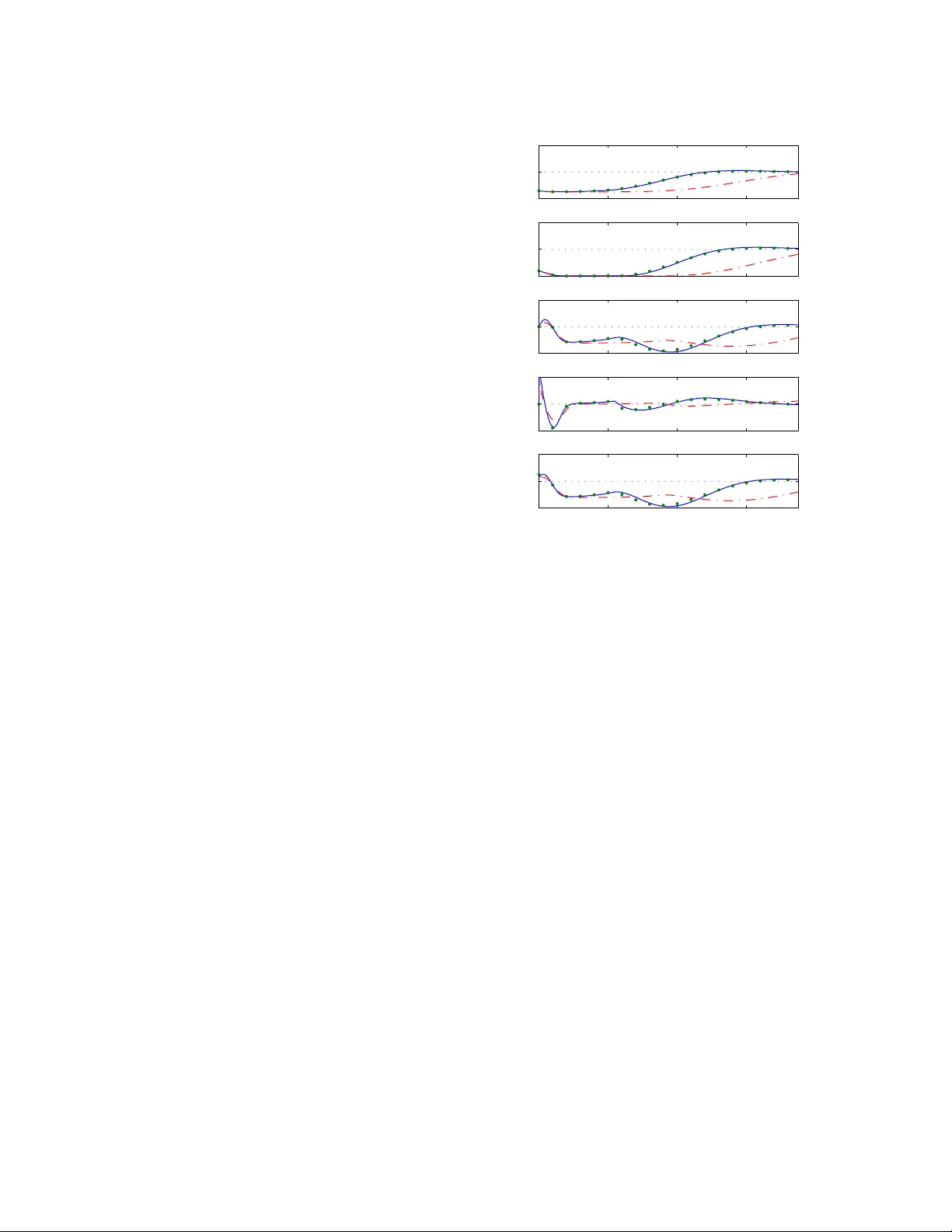
Pro v ably Safe and Robust Learning-Based Mo del Predictiv e Con trol ? Anil Asw ani a , Hum b erto Gonzalez a , S. Shank ar Sastry a , Claire T omlin a a Ele ctric al Engine ering and Computer Scienc es, Berkeley, CA 94720 Abstract Con troller design faces a trade-off betw een robustness and performance, and the reliability of linear con trollers has caused man y practitioners to fo cus on the former. Ho w ever, there is renew ed interest in impro ving system p erformance to deal with gro wing energy constraints. This paper describ es a learning-based mo del predictive con trol (LBMPC) scheme that pro vides deterministic guarantees on robustness, while statistical identification tools are used to iden tify richer mo dels of the system in order to improv e p erformance; the benefits of this framework are that it handles state and input constraints, optimizes system p erformance with respect to a cost function, and can be designed to use a wide v ariety of parametric or nonparametric statistical to ols. The main insight of LBMPC is that safet y and p erformance can b e decoupled under reasonable conditions in an optimization framework by main taining tw o mo dels of the system. The first is an approximate mo del with b ounds on its uncertain t y , and the second mo del is updated by statistical metho ds. LBMPC improv es performance by choosing inputs that minimize a cost sub ject to the learned dynamics, and it ensures safety and robustness by chec king whether these same inputs k eep the approximate model stable when it is sub ject to uncertaint y . F urthermore, we show that if the system is sufficien tly excited, then the LBMPC con trol action probabilistically conv erges to that of an MPC computed using the true dynamics. Key wor ds: Predictiv e con trol; statistics; robustness; safet y analysis; learning con trol. 1 In tro duction T ools from control theory face an inherent trade-off b e- t w een robustness and p erformance. Stabilit y can b e de- riv ed using appro ximate mo dels, but optimalit y requires accurate mo dels. This has driven researc h in adaptive [64,65,55,6,60] and learning-based [74,3,70,1,47] control. Adaptiv e con trol reduces conserv atis m b y mo difying con troller parameters based on system measurements, and learning-based con trol impro ves p erformance b y us- ing measurements to refine models of the system. How- ev er, learning b y itself cannot ensure the prop erties that are imp ortan t to controller safety and stability [15,7,8]. The motiv ation of this paper is to design a con trol sc heme than can (a) handle state and input constraints, (b) optimize system p erformance with resp ect to a cost function, (c) use statistical identification to ols to learn model uncertainties, and (d) prov ably con verge. ? Corresp onding author A. Aswani. Email addr esses: aaswani@eecs.berkeley.edu (Anil Asw ani), hgonzale@eecs.berkeley.edu (Hum berto Gonzalez), sastry@eecs.berkeley.edu (S. Shank ar Sastry), tomlin@eecs.berkeley.edu (Claire T omlin). The main c hallenge is com bining (a) and (c): Statis- tical methods conv erge in a probabilistic sense, and this is not strong enough for the purp ose of providing deterministic guarantees of safet y . Showing (d) is also difficult because of the differences b et ween statistical and dynamical conv ergence. W e introduce a form of robust, adaptive mo del predic- tiv e control (MPC) that we refer to as learning-based mo del predictive control (LBMPC). The main insigh t of LBMPC is that p erformance and safety can be de- coupled in an MPC framew ork by using reac hability to ols [4,14,56,23,5,69,52]. In particular, LBMPC im- pro v es p erformance by c ho osing inputs that minimize a cost sub ject to the dynamics of a learned mo del that is up dated using statistics, while ensuring safety and sta- bilit y b y using theory from robust MPC [19,21,42,44] to c hec k whether these same inputs keep a nominal mo del stable when it is sub ject to uncertaint y . LBMPC is similar to other v ariants of MPC. F or in- stance, linear parameter-v arying MPC (LPV-MPC) has a mo del that changes using successive online lineariza- tions of a nonlinear mo del [38,26]; the difference is that LBMPC up dates the mo dels using statistical metho ds, pro vides robustness to p oor mo del up dates, and can in- v olv e nonlinear mo dels. Other forms of robust, adap- tiv e MPC [28,2] use an adaptive mo del with an uncer- tain t y measure to ensure robustness, while LBMPC uses a learned m odel to improv e p erformance and a nominal mo del with an uncertaint y measure to provide robust- ness. Here, we fo cus on LBMPC for when the nominal mo del is linear and has a known level of uncertaint y . After re- viewing notation and definitions, w e formally define the LBMPC optimization problem. Deterministic theorems ab out safety , stability , and robustness are prov ed. Next, w e discuss ho w learning is incorp orated into the LBMPC framew ork using parametric or nonparametric statisti- cal to ols. Provided sufficient excitation of the system, w e show conv ergence of the control la w of LBMPC to that of an MPC that knows the true dynamics. The pa- p er concludes by discussing applications of LBMPC to three experimental testb eds [12,9,20,13] and to a sim u- lated jet engine compression system [53,25,39]. 2 Preliminaries In this section, we define the notation, the mo del, and summarize three results on estimation and filtering. Note that p olytop es are assumed to b e conv ex and compact. 2.1 Mathematic al Notation W e use A 0 to denote the transp ose of A , and subscripts denote time indices. Marks ab o ve a v ariable distinguish the state, output, and input of different mo dels of the same system. F or instance, the true system has state x , the linear mo del with disturbance has state x , and the mo del with oracle has state ˜ x . A function γ : R + → R + is t yp e- K if it is contin uous, strictly increasing, and γ (0) = 0 [63]. F unction β : R + × R + → R + is type- KL if for each fixed t ≥ 0, the function β ( · , t ) is type- K , and for each fixed s ≥ 0, the function β ( s, · ) is decreasing and β ( s, t ) → 0 as t → ∞ [35]. Also, V m ( x ) is a Ly apunov function for a discrete time system if (a) V m ( x s ) = 0 and V m ( x ) > 0 , ∀ x 6 = x s ; (b) α 1 ( k x − x s k ) ≤ V m ( x ) ≤ α 2 ( k x − x s k ), where α 1 , α 2 are type- K functions; (c) x s lies in this interior of the domain of V m ( x ); and (d) V m +1 ( x m +1 ) − V m ( x m ) < 0 for states x m 6 = x s of a dynamical system. Let U , V , W b e sets. Their Mink o wski sum [66] is U ⊕ V = { u + v : u ∈ U ; v ∈ V } , and their Pon tryagin set differ- ence [66] is U  V = { u : u ⊕ V ⊆ U } . This set difference is not symmetric, and so the order of op erations is im- p ortan t; also, the set difference can result in an empty set. The linear transformation of U b y matrix T is giv en b y T U = { T u : u ∈ U } . Some useful prop erties [66,37] include: ( U  V ) ⊕ V ⊆ U , ( U  ( V ⊕ W )) ⊕ W ⊆ U  V , ( U  V )  W ⊆ U  ( V ⊕ W ), and T ( U  V ) ⊆ T U  T V . F or a sequence f n and rate r n , the notation f n = O ( r n ) means that ∃ M , N > 0 suc h that k f n k ≤ M k r n k , for all n > N . F or a random v ariable f n , constant f , and rate r n , the notation k f n − f k = O p ( r n ) means that given  > 0, ∃ M , N > 0 such that P ( k f n − f k /r n > M ) <  , for all n > N . The notation f n p − → f means that there exists r n → 0 suc h that k f n − f k = O p ( r n ). 2.2 Mo del Let x ∈ R p b e the state vector, u ∈ R m b e the con trol input, and y ∈ R q b e the output. W e assume that the states x ∈ X and control inputs u ∈ U are constrained b y the p olytop es X , U . The true system dynamics are x n +1 = Ax n + B u n + g ( x n , u n ) (1) and y n = C x n , where A, B , C are matrices of appro- priate size and g ( x, u ) describes the unmo deled (p ossi- bly nonlinear) dynamics. The in tuition is that w e ha v e a nominal linear mo del with mo deling error. The term un- certain t y is used interc hangeably with mo deling error. W e assume that the mo deling error g ( x, u ) of (1) is b ounded and lies within a p olytope W , meaning that g ( x, u ) ∈ W for all ( x, u ) ∈ ( X , U ). This assumption is not restrictive in practice b ecause it holds whenev er g ( x, u ) is contin uous, since X , U are bounded. Moreov er, the set W can b e determined using techniques from un- certain t y quan tification [18]; for example, the residual error from mo del fitting can b e used to compute this uncertain t y . 2.3 Estimation and Filtering Sim ultaneously performing state estimation and learn- ing unmo deled dynamics requires measuring all states [10], except in sp ecial cases [9]. W e fo cus on the case in which all states are measured (i.e, C = I ). It is p os- sible to relax these assumptions by using set theoretic estimation metho ds (e.g., [51]), but we do not consider those extensions here. F or simplicit y of presen tation, w e assume that there is no measurement noise; ho wev er, our results extend to the case with measuremen t noise b y simply replacing the modeling error W in our results with W ⊕ D , where D is a polytop e encapsulating the effect of b ounded measurement noise. 3 Learning-Based MPC This section presen ts the LBMPC technique. The first step is to use reachabilit y to ols to construct a terminal set with robustness prop erties for the LBMPC, and this terminal set is important for proving the stabilit y , safet y , and robustness prop erties of LBMPC. The terminal con- strain t set is t ypically used to guaran tee both feasibility 2 and con vergence [50]. W e decouple p erformance from ro- bustness by iden tifying feasibility with robustness and con v ergence with p erformance. One no velt y of LBMPC is that differen t models of the system are maintained b y the controller. In order to de- lineate the v ariables of the v arious mo dels, we add marks ab o ve x and u . The true system (1) has state x and in- put u . The nominal linear mo del with uncertain t y has state x and input u ; its dynamics are given by x n +1 = Ax n + B u n + d n , (2) where d n ∈ W is a disturbance. Because g ( x, u ) ∈ W , the d n reflects the uncertain nature of mo deling error. F or the learned model, w e denote the state ˜ x and input ˜ u . Its dynamics are ˜ x n +1 = A ˜ x n + B ˜ u n + O n ( ˜ x n , ˜ u n ), where O n is a time-v arying function that is called the oracle. The reason we call this function the oracle is in reference to computer science in which an oracle is a black b o x that tak es in inputs and giv es an answer: LBMPC only needs to know the v alue (and gradient when doing numerical computations) of this function at a finite set of p oin ts; and yet, the mathematical structure and details of how the oracle is computed are not relev ant to the stability and robustness prop erties of LBMPC. 3.1 Construction of an Invariant Set W e b egin by recalling tw o facts [44]. First, if ( A, B ) is sta- bilizable, then the set of steady-state p oin ts are x s = Λ θ and u s = Ψ θ , where θ ∈ R m and Λ , Ψ are full column- rank matrices with suitable dimensions. These matrices can b e computed with a n ull space computation, b y not- ing that range([Λ 0 Ψ 0 ] 0 ) = null([( I − A ) − B ]). Second, if ( A + B K ) is Sc hur stable (i.e., all eigen v alues ha ve magnitude strictly less than one), then the con trol input u n = K ( x n − x s ) + u s = K x n + (Ψ − K Λ) θ steers (2) to steady-state x s = Λ θ and u s = Ψ θ , whenever d n ≡ 0. These facts are useful b ecause they can b e used to con- struct a robust reac hable set that serves as the terminal constrain t set for LBMPC. The particular type of reach set w e use is kno wn as a maximal output admissible dis- turbance inv ariant set Ω ⊆ X × R m . It is a set of p oin ts suc h that an y tra jectory of the system with initial con- dition chosen from this set and with control u n remains within the set for any sequence of b ounded disturbance, while satisfying constraints on the state and input [37]. These prop erties of Ω are formalized as (a) constraint satisfaction: Ω ⊆ { ( x, θ ) : x ∈ X ; Λ θ ∈ X ; K x + (Ψ − K Λ) θ ∈ U ; Ψ θ ∈ U } , (3) and (b) disturbance inv ariance: " A + B K B (Ψ − K Λ) 0 I # Ω ⊕ ( W × { 0 } ) ⊆ Ω . (4) Recall that the θ comp onen t of the set is a parametriza- tion of which p oin ts can b e track ed using control u n . The set Ω has an infinite num b er of constraints in gen- eral, though arbitrarily goo d approximations can be computed in a finite n umber of steps [37,44,57]. These appro ximations maintain b oth disturbance inv ariance and constrain t satisfaction, and these are the prop erties whic h are used in the pro ofs for our MPC scheme. So ev en though our results are for Ω, they equally hold true for appropriately computed approximations. 3.2 Stability and Safety of LBMPC LBMPC uses tec hniques from a type of robust MPC kno wn as tube MPC [21,42,44], and it enlarges the fea- sible domain of the con trol b y using trac king ideas from [22,45]. The idea of tub e MPC is that given a nominal tra jectory of the linear system (2) without disturbance, then the tra jectory of the true system (1) is guaranteed to lie within a tube that surrounds the nominal tra jec- tory . A linear feedback K is used to control ho w wide this tub e can grow. Moreo ver, LBMPC fixes the initial condition of the nominal tra jectory as in [21,42], as op- p osed to letting the initial condition b e an optimization v ariable as in [44]. Let N b e the n umber of time steps for the horizon of the MPC. The width of the tub e at the i -th step, for i ∈ I = { 0 , . . . , N − 1 } , is given b y a set R i , and the constrain ts X are shrunk by the width of this tub e. The result is that if the nominal tra jectory lies in X  R i , then the true tra jectory lies in X . Similarly , supp ose that the N - th step of the nominal tra jectory lies in Pro j x (Ω)  R N , where Pro j x (Ω) = Ω x = { x : ∃ θ s.t. ( x, θ ) ∈ Ω } ; then the true tra jectory lies in Pro j x (Ω), and the in v ariance prop erties of Ω imply that there exists a con trol that k eeps the system stable even under disturbances. The following optimization problem defines LBMPC V n ( x n ) = min c,θ ψ n ( θ , ˜ x n , . . . , ˜ x n + N , ˇ u n , . . . , ˇ u n + N − 1 ) (5) sub ject to: ˜ x n = x n , x n = x n (6) ˜ x n + i +1 = A ˜ x n + i + B ˇ u n + i + O n ( ˜ x n + i , ˇ u n + i ) (7) x n + i +1 = Ax n + i + B ˇ u n + i ˇ u n + i = K x n + i + c n + i x n + i +1 ∈ X  R i , ˇ u n + i ∈ U  K R i ( x n + N , θ ) ∈ Ω  ( R N × { 0 } )        (8) 3 for all i ∈ I in the constraints; K is the feedbac k gain used to compute Ω; R 0 = { 0 } and R i = L i − 1 j =0 ( A + B K ) j W ; O n is the oracle; and ψ n are non-negativ e func- tions that are Lipsc hitz con tinuous in their argumen ts. Note that the Lipschitz assumption is not restrictive b e- cause it is satisfied by costs with b ounded deriv ativ es; for example, linear and quadratic costs satisfy this due to the b oundedness of states and inputs. Also note that the same con trol ˇ u [ · ] is applied to b oth the nominal and learned mo dels. R emark 1 . The cost ψ n is a function of the states of the learned mo del, whic h uses the oracle to up date the nominal mo del. The cost function may con tain a termi- nal cost, an offset cost, a stage cost, etc. An in teresting feature of LBMPC is that its stabilit y and robustness prop erties do not dep end on the actual terms within the cost function; this is one of the reasons that w e state that LBMPC decouples safety (i.e., stability and robustness) from p erformance (i.e., having the cost b e a function of the learned mo del). R emark 2 . The constrain ts in (8) are tak en from [21] and are robustly imposed on the nominal linear model (2), taking in to accoun t the prior bounds on the unmo d- eled dynamics of the nominal model g ( x, u ). The reason that the constraints are not relaxed to exploit the refined results of the oracle (as in [28,2]) is that this provides robustness to the situation in which the learned model is not a go od representation of the true dynamics. It is known that the p erformance of a learning-based con- troller can b e arbitrarily bad if the learned mo del do es not exactly match the true mo del [15]; imp osing the con- strain ts on the nominal mo del, instead of the learned mo del, protects against this situation. R emark 3 . There is another, more subtle reason for main taining tw o mo dels. Suppose that the oracle is b ounded b y a p olytope O n ∈ P , where P is a p olytope; then, the worst case error b et ween the true model (1) and the learned mo del (7) lies within the polytop e W ⊕ P , whic h is strictly larger than W whenev er P 6 = { 0 } . In tuitiv ely , this me an s that if we were to use the worst- case bounded learned mo del in the constrain ts, then the constrain ts will be reduced by a larger amount W ⊕ P ; this is in contrast to using the nominal mo del in which case the constraints are reduced by only W . Note that the v alue function V n ( x n ) (i.e., the v alue of the ob jective (5) at its minim um), the cost function ψ n , and the oracle O n can be time-v arying b ecause they are functions of n . It is imp ortan t that the oracle b e allow ed to b e time-v arying, b ecause it is up dated using statistical metho ds as time adv ances and more data is gathered. This is discussed in more detail in the next section. Let M n b e a feasible p oin t for the LBMPC scheme (5) with initial state x n , and denote a minimizing p oin t of (5) as M ∗ n . The states and inputs predicted by the lin- ear mo del (2) for p oin t M n are denoted x n + i [ M n ] and u m + n [ M n ], for i ∈ I . In this notation, the con trol law is explicitly given by u m [ M ∗ n ] = K x n + c n [ M ∗ n ] . (9) This MPC scheme is endo w ed with robust feasibilit y and constrain t satisfaction prop erties, which in turn imply stabilit y of the closed-lo op control pro vided b y LBMPC. The equiv alence b et ween these prop erties and stability holds b ecause of the compactness of constraints X , U . Theorem 1. If Ω has the pr op erties define d in Se ct. 3.1 and M n = { c n , . . . , c n + N − 1 , θ n } is fe asible for the LBMPC scheme (5) with x n , then applying the c ontr ol (9) gives a) R obust fe asibility: ther e exists a fe asible M n +1 for x n +1 ; b) R obust c onstr aint satisfaction: x n +1 ∈ X . Pr o of. The pro of follows a similar line of reasoning as Lemma 7 of [21]. W e b egin b y showing that the following p oin t M n +1 = { c n +1 , . . . , c n + N − 1 , 0 , θ n } is feasible for x n +1 ; the results follow as consequences of this. Let d n +1+ i [ M n ] = ( A + B K ) i g ( x n , u n ), and note that d n +1+ i [ M n ] ∈ ( A + B K ) i +1 W . Some algebra giv es the predicted states for i = 0 , . . . , N − 1 as x n +1+ i [ M n +1 ] = x n +1+ i [ M n ] + d n +1+ i [ M n ] and pre- dicted inputs for i = 0 , . . . , N − 2 as ˇ u n +1+ i [ M n +1 ] = ˇ u n +1+ i [ M n ] + K d n +1+ i [ M n ]. Because M n is feasible, this means b y definition that x n +1+ i [ M n ] ∈ X  R i +1 for i = 0 , . . . , N − 1. Com bining terms giv es x n +1+ i [ M n +1 ] ∈ X  ( R i ⊕ ( A + B K ) i +1 W ) ⊕ ( A + B K ) i +1 W . It follo ws that x n +1+ i [ M n +1 ] ∈ X  R i for i = 0 , . . . , N − 1. Simi- lar reasoning giv es that ˇ u n +1+ i [ M n +1 ] ∈ U  K R i for i = 0 , . . . , N − 2. The same argument gives ( x n +1+ N − 1 [ M n +1 ] , θ n ) ∈ Ω  ( R N − 1 × { 0 } ) ⊂ Ω . Now by construction of M n +1 , it holds that ˇ u n +1+ N − 1 [ M n +1 ] = M p , where M = [ K (Ψ − K Λ)] is a matrix and p = ( x n +1+ N − 1 [ M n +1 ] , θ n ) is a p oin t. Therefore, we ha ve ˇ u n +1+ N − 1 [ M n +1 ] = M p ⊆ M Ω  M ( R N − 1 × { 0 } ) = M Ω  K R N − 1 . Ho wev er, the constraint satisfaction prop ert y of Ω (3) implies that M Ω ⊆ U . Consequently , w e hav e that ˇ u n +1+ N − 1 [ M n +1 ] ∈ U  K R N − 1 . Next, observ e that the con trol ˇ u n +1+ N − 1 [ M n +1 ] leads to x n +1+ N [ M n +1 ] = ([ A 0] + B M ) p . Consequently , w e hav e x n +1+ N [ M n +1 ] ∈ ([ A 0] + B M )Ω  ( A + B K ) R N − 1 . As a result of the disturbance inv ariance prop ert y of Ω (4), it m ust be that ( x n +1+ N [ M n +1 ] , θ n ) ∈ (Ω  ( W × { 0 } ))  (( A + B K ) R N − 1 × { 0 } ) = Ω  ( R N × { 0 } ). This completes the pro of for part (a). 4 Similar arithmetic shows that the true, next state is x n +1 [ M n ] = x n +1 [ M n ] + w n where w n = g ( x n , u n ) ∈ W . Since M n is a feasible p oin t, it holds that x n +1 [ M n ] ∈ X  W . This implies that x n +1 [ M n ] = x n +1 [ M n ] + w n ∈ ( X  W ) ⊕ W ⊆ X ; this pro ves part (b). Corollary 1. If Ω has the pr op erties define d in Se ct. 3.1 and M 0 is fe asible for the LBMPC scheme (5) with initial state x 0 , then the close d-lo op system pr ovide d by LBMPC is (a) stable, (b) satisfies al l state and input c onstr aints, and (c) fe asible, for al l p oints of time n ≥ 0 . R emark 4 . Robust feasabilit y and constraint satisfac- tion, as in Theorem 1, trivially imply this result. R emark 5 . These results apply to the case where ψ n , O n are time-v arying; this allows, for example, changing the set p oin t of the LBMPC using the approac h in [45]. Moreo v er, the safet y and stability that w e hav e prov ed for the closed-lo op system under LBMPC are actually robust results b ecause they imply that the states remain within bounded constraints even under disturbances, pro vided the mo deling error in (2) follows the prescribed b ound and the inv ariant set Ω can b e computed. Next, w e discuss additional t yp es of robustness pro- vided b y LBMPC. First, w e sho w that the v alue func- tion V n ( x n ) of LBMPC (5) is contin uous, and this prop- ert y can b e used for establishing certain other types of robustness of an MPC controller [30,48,58,43]. Lemma 1. L et X F = { x n : ∃M n } b e the fe asible r e gion of the LBMPC (5). If ψ n , O n ar e c ontinuous, then V n ( x n ) is c ontinuous on int ( X F ) . Pr o of. W e define a cost function ˜ ψ n and constrain t func- tion φ such that the LBMPC (5) can b e rewritten as min c,θ ˜ ψ n ( θ , x n , c n , . . . , c n + N − 1 ) s.t. ( c, θ ) ∈ φ ( x n ) . (10) The pro of pro ceeds by showing that b oth the ob jective ˜ ψ n and constrain t φ are contin uous. Under suc h con- tin uit y , we get contin uity of the v alue function by the Berge maxim um theorem [16] (or equiv alen tly b y Theo- rem C.34 of [58]). Because the constraints (6) and (8) in LBMPC are lin- ear, the constrain t φ is con tinuous [30]. Contin uity of ˜ ψ n follo ws by noting that it is the comp osition of con tinu- ous functions — specifically (5), (6), and (7) — is also a con tin uous function [61]. R emark 6 . This result is surprising b ecause a non- con v ex (and hence nonlinear) MPC problem generally has a discontin uous v alue function (cf. [30]). LBMPC is non-con v ex when O n is nonlinear (or ψ n is non-con vex), and the reason that w e ha v e a contin uous v alue function is that our active constrain ts are linear equality con- strain ts or p olytopes. In practice, this result requires b eing able to numerically compute a global minimum, and this can only b e efficiently done for con vex opti- mization problems. R emark 7 . The pro of of this result suggests another b en- efit of LBMPC: The fact that the constraints are linear means that suboptimal solutions can be computed by solving a linear (and hence conv ex) feasibility problem, ev en when the LBMPC problem is nonlinear. This en- ables more precise tradeoffs b et ween computation and solution accuracy , as compared to conv entional forms of nonlinear MPC. Next, w e pro ve that LBMPC is robust b ecause its w orst case b eha vior is an increasing function of mo deling error. This type of robustness if formalized by the follo wing definition. Definition 1 (Grimm, et al. [30]) . A system is robustly asymptotically stable (RAS) ab out x s if there exists a t yp e- KL function β and for each  > 0 there exists δ > 0, suc h that for all d n satisfying max n k d n k < δ it holds that x n ∈ X and k x n − x s k ≤ β ( k x 0 − x s k , n ) +  for all n ≥ 0. R emark 8 . The intuition is that if a controller for the appro ximate system (2) with no disturbance conv erges to x s , then the same controller applied to the appro x- imate system (2) with b ounded disturbance (note that this also includes the true system (1)) asymptotically remains within a b ounded distance from x s . W e can no w pro v e when LBMPC is RAS. The key in tu- itiv e p oin ts are that linear MPC (i.e, LBMPC with an iden tically zero oracle: O n ≡ 0) needs to b e prov ably con v ergent for the approximate mo del with no distur- bance, and the oracle for LBMPC needs to be b ounded. Theorem 2. Assume (a) Ω has the pr op erties define d in Se ct. 3.1; (b) M 0 is fe asible for LBMPC (5) with x 0 ; (c) the c ost function ψ n is time-invariant, c ontinuous, and strictly c onvex, and (d) ther e exists a c ontinuous Lya- punov function W ( x ) for the appr oximate system (2) with no disturb anc e, when using the c ontr ol l aw of line ar MPC (i.e, LBMPC with O n ≡ 0 ). Under these c onditions, the c ontr ol law of LBMPC is RAS with r esp e ct to the distur- b anc e d n in (2), whenever the or acle O n is a c ontinuous function satisfying max n, X ×U kO n k ≤ δ . Note that this δ is the same one as fr om the definition of RAS. Pr o of. Let M ∗ n b e the minimizer for linear MPC, and note that it is unique b ecause ψ n is assumed to b e strictly con v ex. Similarly , let M ∗ n b e a minimizer for LBMPC. No w consider the state-dep enden t disturbance e n = B ( ˇ u n [ M ∗ n ] − ˇ u n [ M ∗ n ]) + d n , (11) 5 for the approximate system (2). By construction, it holds that x n +1 [ M ∗ n ] = x n +1 [ M ∗ n ] + e n . Prop osition 8 of [30] and Theorem 1 imply that given  > 0, there exists δ 1 > 0 such that for all e n satisfying max n k e n k < δ 1 it holds that x n ∈ X and k x n − x s k ≤ β ( k x 0 − x s k , n ) +  for all n ≥ 0. What remains to b e c hec ked is whether there exists δ suc h that max n k e n k < δ 1 for the e n defined in (11). The same argumen t as used in Lemma 1 coupled with the strict con v exity of the linear MPC gives that M ∗ n is con tin uous, with resp ect to O n , when O n ≡ 0. (Re- call that the minimizer at this p oin t is M ∗ n .) Because of this contin uity , this means that there exists δ 2 > 0 suc h that k ˇ u n [ M ∗ n ] − ˇ u n [ M ∗ n ] k ≤ δ 1 / (2 k B k ), whenever the oracle lies in the set {O n : kO n k < δ 2 } . T aking δ = min { δ 1 / 2 , δ 2 } giv es the result. R emark 9 . Condition (a) is satisfied if the set Ω can b e computed; it cannot be computed in some situations be- cause it is p ossible to hav e Ω = ∅ . Conditions (b) and (c) are easy to c heck. As w e will sho w in Sect. 3.2.1, certain systems hav e easy sufficien t conditions for chec king the Ly apuno v conditions in (d). 3.2.1 Example: T r acking in Line arize d Systems Here, we show that the Lyapuno v condition in The- orem 2 can b e easily chec ked when the cost function is quadratic and the approximate mo del is linear with b ounds on its uncertaint y . Suppose we use the quadratic cost defined in [45] ψ n = k ˜ x n + N − Λ θ k 2 P + k x s − Λ θ k 2 T + P N − 1 i =0 k ˜ x n + i − Λ θ k 2 Q + k ˇ u n + i − Ψ θ k 2 R , (12) where P , Q, R, T are p ositiv e definite matrices, to track to the p oin t x s ∈ { Λ θ : Λ θ ∈ X } . Then, the Lyapuno v condition required for Theorem 2 holds. Prop osition 1. F or line ar MPC with c ost (12) wher e x s ∈ { Λ θ : Λ θ ∈ X } is kept fixe d, if ( A + B K ) is Schur stable and P solves the discr ete-time Lyapunov e quation ( A + B K ) 0 P ( A + B K ) − P = − ( Q + K 0 RK ) ; then ther e exists a c ontinuous Lyapunov function W for the e qui- librium p oint x s of the appr oximate mo del (2) with no disturb anc es. Pr o of. First note that b ecause w e consider the linear MPC case, we hav e by definition ˜ x = x . Results from con verse Lyapuno v theory [36] indicate that the result is true if the following t wo conditions hold. The first is lo cal uniform stability , meaning that for every  > 0, there exists some δ > 0 such that k x 0 − x s k < δ implies that k x n − x s k <  for all n ≥ 0. The second is that lim n →∞ k x n − x s k = 0 for all feasible p oin ts x 0 ∈ X F . The second condition w as sho wn in Theorem 1 of [45], and so we only need to chec k the first condition. W e b egin b y noting that since Q, T are p ositiv e definite matrices, there exists a positive definite matrix S suc h that S < Q and S < T . Next, observ e that k ˜ x n − x s k 2 S ≤ k ˜ x n − Λ θ k 2 Q + k x s − Λ θ k 2 T ≤ ψ n . Minimizing the b oth sides of the inequality sub ject to the linear MPC constraints yields k ˜ x n − x s k 2 S ≤ V ( x n ), where V ( x n ) is the v alue function of the linear MPC optimization. Because linear MPC is the sp ecial case of LBMPC in whic h O n ≡ 0, the result in Lemma 1 applies: The v alue function V ( x n ) is con tinuous. F urthermore, the pro of of Theorem 1 of [45] shows that the v alue function is non- increasing (i.e., V ( x n +1 )) ≤ V ( x n )), non-negativ e (i.e., V ( x n ) ≥ 0), and zero-v alued only at the equilibrium p oin t (i.e., V ( x s ) = 0). Because of the contin uity of the v alue function, given  > 0 there exists δ > 0, suc h that V ( x 0 ) <  whenever k x 0 − x s k < δ . The lo cal uniform stabilit y condition holds by noting that k ˜ x n − x s k 2 S ≤ V ( x n ) ≤ V ( x 0 ) =  , and this prov es the result. R emark 10 . The result do es not immediately follow from [45], b ecause the v alue function of the linear MPC is not a Ly apunov function in this situation. In particular, the v alue function is non-increasing, but it is not strictly decreasing. 4 The Oracle In theoretical computer science, oracles are black boxes that take in inputs and giv e answers. An imp ortan t class of argumen ts kno wn as relativizing proofs utilize oracles in order to prov e results in complexity theory and com- putabilit y theory . These pro ofs pro ceed b y endo wing the oracle with certain generic properties and then studying the resulting consequences. W e ha ve named the functions O n oracles in reference to those in computer science. Our reason is that w e pro v ed robustness and stability prop erties of LBMPC b y only assuming generic prop erties, such as contin uity or b oundedness, on the function O n . These functions are arbitrary , which can include w orst case behavior, for the purp ose of the theorems in the previous section. Whereas the previous section considered the oracles as abstract ob jects, here w e discuss and study sp ecific forms that the oracle can tak e. In particular, we can design O n to b e a statistical to ol that identifies b etter system mo dels. This leads to tw o natural questions: First, what are examples of statistical metho ds that can b e used to construct an oracle for LBMPC? Secondly , when do es 6 the control la w of LBMPC conv erge to the control la w of MPC that knows the true mo del? This section b egins by defining t wo general classes of sta- tistical to ols that can b e used to design the oracle O n . F or concreteness, w e pro vide a few examples of metho ds that belong to these tw o classes. The section concludes b y addressing the second question ab o ve. Because our con trol law is the minimizer of an optimization problem, the key technical issue that we discuss is sufficient con- ditions that ensure conv ergence of the minimizers of a sequence of optimization problems to the minimizer of a limiting optimization problem. 4.1 Par ametric Or acles A parametric oracle is a con tinuous function O n ( x, u ) = χ ( x, u ; λ n ) that is parameterized by a set of co efficien ts λ n ∈ T ⊆ R L , where T is a set. This class of learning is often used in adaptiv e control [64,6]. In the most general case, the function χ is nonlinear in all its argume n ts, and it is customary to use a least-squares cost function with input and tra jectory data to estimate the parameters ˆ λ n = arg min λ ∈T P n j =0 ( Y j − χ ( x j , u j ; λ )) 2 , (13) where Y i = x i +1 − ( Ax i + B u i ). This can b e difficult to compute in real-time b ecause it is generally a nonlinear optimization problem. Example 1 . It is common in biochemical netw orks to ha v e nonlinear terms in the dynamics such as O n ( x, u ) = λ n, 1 x λ n, 2 1 x λ n, 2 1 + λ n, 3 ! λ n, 4 u λ n, 5 1 + λ n, 4 ! , (14) where λ n ∈ T ⊂ R 5 are the unkno wn co efficien ts in this example. Such terms are often called Hill equation type reactions [11]. An imp ortan t sub class of parametric oracles are those that are linear in the co efficien ts: O n ( x, u ) = P L i =1 λ n,i χ i ( x, u ), where χ i ∈ R p for i = 1 , . . . , L are a set of (p ossibly nonlinear) functions. The reason for the imp ortance of this sub class is that the least-squares pro cedure (13) is conv ex in this situation, even when the functions χ i are nonlinear. This greatly simplifies the computation required to solve the least-squares problem (13) that gives the unknown co efficien ts λ n . Example 2 . One sp ecial case of linear parametric ora- cles is when the χ i are linear functions. Here, the ora- cle can b e written as O m ( x, u ) = F λ m x + G λ m u , where F λ m , G λ m are matrices whose entries are parameters. The in tuition is that this oracle allo ws for corrections to the v alues in the A, B matrices of the nominal mo del; it was used in conjunction with LBMPC on a quadro- tor helicopter testb ed [9,20], in which LBMPC enabled high-p erformance fligh t. 4.2 Nonp ar ametric Or acles Nonparametric regression refers to techniques that esti- mate a function g ( x, u ) of input v ariables suc h as x, u , without making a priori assumptions ab out the mathe- matical form or structure of the function g . This class of tec hniques is in teresting b ecause it allo ws us to integrate non-traditional forms of adaptation and “learning” into LBMPC. And b ecause LBMPC robustly maintains fea- sibilit y and constraint satisfaction as long as Ω can b e computed, we can design or choose the nonparametric regression metho d without having to w orry ab out stabil- it y properties. This is a specific instantiation of the sepa- ration b et ween robustness and p erformance in LBMPC. Example 3 . Neural netw orks are a classic example of a nonparametric method that has been used in adap- tiv e con trol [55,60,3], and they can also be used with LBMPC. There are many particular forms of neural net- w orks, and one specific type is a feedforw ard neural net- w ork with a hidden lay er of k n neurons; it is given by O n ( x, u ) = c 0 + P k n i =1 c i σ ( a 0 i [ x 0 u 0 ] 0 + b i ) , (15) where a i ∈ R p + m and b i , c 0 , c i ∈ R for all i ∈ { 1 , . . . , k } are co efficien ts, and σ ( x ) = 1 / (1 + e − x ) : R → [0 , 1] is a sigmoid function [31]. Note that this is considered a nonparametric metho d because it do es not generally con v erge unless k n → ∞ as n → ∞ . Designing a nonparametric oracle for LBMPC is chal- lenging b ecause the tool should ideally b e an estimator that is b ounded to ensure robustness of LBMPC and dif- feren tiable to allow for its use with numerical optimiza- tion algorithms. Lo cal linear estimators [62,8] are not guaran teed to b e bounded, and their extensions that re- main b ounded are generally non-differentiable [27]. On the other hand, neural net works can b e designed to re- main b ounded and differentiable, but they can hav e tech- nical difficulties related to the estimation of its co effi- cien ts [72]. 4.2.1 Example: L 2 -R e gularize d Nadar aya-Watson Es- timator The Nadara ya-W atson (NW) estimator [54,62], whic h can b e intuitiv ely thought of as the in terp olation of non- uniformly sampled data p oin ts by a suitably normal- ized conv olution kernel, is promising because it ensures b oundedness. Our approach to designing a nonparamet- ric estimator for LBMPC is to mo dify the NW estimator b y adding regularization that deterministically ensures b oundedness. Th us, it serves the same purp ose as trim- ming [17]; but the benefit of our approac h is that it also deterministically ensures differentiabilit y of the estima- tor. T o our knowledge, this mo dification of NW has not b een previously considered in the literature. 7 Define h n , λ n ∈ R + to b e tw o non-negative parameters; except when we wish to emphasize their temp oral de- p endence, w e will drop the subscript n to match the con v ention of the statistics literature. Let X i = [ x 0 i u 0 i ] 0 , Y i = x i +1 − ( Ax i + B u i ), and Ξ i = k ξ − x i k 2 /h 2 , where X i ∈ R p + m and Y i ∈ R p are data and ξ = [ x 0 u 0 ] 0 are free v ariables. W e define any function κ : R → R + to be a k ernel function if it has (a) finite supp ort (i.e., κ ( ν ) = 0 for | ν | ≥ 1), (b) even symmetry κ ( ν ) = κ ( − ν ), (c) p os- itiv e v alues κ ( ν ) > 0 for | ν | < 1, (d) differentiabilit y (denoted by dκ ), and (e) nonincreasing v alues of κ ( ν ) o v er ν ≥ 0. The L 2-regularized NW (L2NW) estimator is defined as O n ( x, u ) = P i Y i κ (Ξ i ) λ + P i κ (Ξ i ) , (16) where λ ∈ R + . If λ = 0, then (16) is simply the NW estimator. The λ term acts to regularize the problem and ensures differentiabilit y . There are t wo alternativ e characterizations of (16). The first is as the unique minimizer of the parametrized, strictly conv ex optimization problem O n ( x, u ) = arg min γ L ( x, u, X i , Y i , γ ) for L ( x, u, X i , Y i , γ ) = P i κ (Ξ i )( Y i − γ ) 2 + λγ 2 . (17) View ed in this wa y , the λ term represents a Tikhonov (or L 2) regularization [71,32]. The second characteriza- tion is as the mean with w eights { λ, κ (Ξ 1 ) , . . . , κ (Ξ n ) } for points { 0 , Y 1 , . . . , Y n } , and it is useful for showing the second part of the follo wing theorem ab out the de- terministic prop erties of the L2NW estimator. Theorem 3. If 0 ∈ W , κ ( · ) is a kernel function, and λ > 0 ; then (a) the L2NW estimator O n ( x, u ) as define d in (16) is differ entiable, and (b) O n ( x, u ) ∈ W . Pr o of. T o prov e (a), note that the estimate O n ( x, u ) is the v alue of γ that solves dL dγ ( x, u, X i , Y i , γ ) = 0, where L ( · ) is from (17). Because λ + P i κ (Ξ i ) > 0, the h yp oth- esis of the implicit function theorem is satisfied, and re- sult directly follo ws from the implicit function theorem. P art (b) is shown by noting that the assumptions im- ply that 0 , Y i ∈ W . If the weigh ts of a weigh ted mean are p ositiv e and hav e a nonzero sum, then the weigh ted mean can b e written as a con vex com bination of p oin ts. This is our situation, and so the result follo w from the w eigh ted mean characterization of (16). R emark 11 . This sho ws that L2NW is deterministically b ounded and differentiable, whic h is needed for robust- ness and n umerical optimization, resp ectiv ely . W e can compute the gradien t of L2NW using standard calculus, and its j k -th comp onen t is giv en by (18) for fixed X i , Y i . There are few notes regarding n umerical computation of L2NW. First, pic king the parameters λ, h in a data- driv en manner [24,67] is to o slo w for real-time imple- men tation, and so we suggest rules of thum b: Deter- ministic regularity is pro vided by Theorem 3 for an y p ositiv e λ (e.g., 1e-3), and we conjecture using h n = O ( n − 1 / ( p + m ) ) b ecause random samples cov er X × U ⊆ R p + m at this rate. Second, computational savings are p ossible through careful soft ware co ding, because if h is small, then most terms in the summations of (17) and (18) will b e zero b ecause of the finite supp ort of κ ( · ). 4.3 Sto chastic Epi-c onver genc e It remains to be shown that if O n ( x, u ) sto c hastically con v erges to the true model g ( x, u ), then the control la w of the LBMPC scheme will sto c hastically con verge to that of an MPC that knows the true mo del. The main tec hnical problem o ccurs because O n is time-v arying, and so the con trol law is given by the minimizer of an LBMPC optimization problem that is differen t at eac h p oin t in time n . This presents a problem b ecause point- wise con vergence of O n to g is generally insufficien t to pro v e con vergence of the minimizers of a sequence of op- timization problems to the minimizer of a limiting opti- mization problem [59,73]. A related notion called epi-conv ergence is sufficient for sho wing conv ergence of the control law. Define the epi- gr aph of f n ( · , ω ) to b e the set of all p oin ts lying on or ab o ve the function, and denote it as Epi f n ( · , ω ) = { ( x, µ ) : µ ≥ f n ( x, ω ) } . T o prov e con v ergence of the se- quence of minimizers, we m ust show that the epigraph of the cost function (and constraints) of the sequence of optimizations c on v erges in probability to the epigraph of the cost function (and constraints) in the limiting opti- mization problem. This notion is called epi-con vergence, and we denote it as f n l − pr ob. − − − − − → X f 0 . F or simplicit y , w e will assume in this section that the cost function is time-inv arian t (i.e., ψ n ≡ ψ 0 ). It is enough to cite the relev ant results for our purp oses, but the in- terested reader can refer to [59,73] for details. Theorem 4 (Theorem 4.3 [73]) . L et ˜ ψ n and φ b e as define d in L emma 1, and define ˜ ψ 0 to b e the c omp osition of (5) with b oth (6) and x n + i +1 ( x n + i , u n + i ) = Ax n + i + B u n + i + g ( x n + i , u n + i ) . If ˜ ψ n l − pr ob. − − − − − → φ ( x n ) ˜ ψ 0 for al l { x n : φ ( x n ) 6 = ∅} , then the set of minimizers c onver ges arg min { ˜ ψ n | ( c, θ ) ∈ φ ( x n ) } p − → arg min { ˜ ψ 0 | ( c, θ ) ∈ φ ( x n ) } . (19) R emark 12 . The in tuition is that if the cost function ψ n comp osed with the oracle O n ( x, u ) conv erges in the ap- 8 ∂ O n ∂ ξ k  x, u  = { P i [ Y i ] j · dκ (Ξ i ) · Ξ i · [ ξ − X i ] k }{ λ + P i κ (Ξ i ) } − { P i [ Y i ] j κ (Ξ i ) }{ P i dκ (Ξ i ) · Ξ i · [ ξ − X i ] k } h 2 { λ + P i κ (Ξ i ) } 2 / 2 . (18) propriate manner to ψ 0 comp osed with the true dynam- ics g ( x, u ); then w e get con v ergence of the minimizers of LBMPC to those of the MPC with true mo del, and the con trol law (9) conv erges. This theorem can b e used to pro v e conv ergence of the LBMPC control law. 4.4 Epi-c onver genc e for Par ametric Or acles Sufficien t excitation (SE) is an imp ortan t concept in sys- tem identification, and it in tuitively means that the con- trol inputs and state tra jectory of the system are such that all modes of the system are activ ated. In general, it is hard to design a control sc heme that ensures this a priori , whic h is a key aim of reinforcemen t learning [15]. Ho w ever, LBMPC pro vides a framework in whic h SE ma y b e able to b e designed. Because w e hav e a nominal mo del, w e can in principle design a reference tra jectory that sufficiently explores the state-input space X × U . Though designing a controller that ensures SE can b e difficult, chec king a p osteriori whether a system has SE is straightforw ard [46,7,8]. In this section, we assume SE and leav e op en the problem of ho w to design reference tra jectories for LBMPC that guarantee SE. This is not problematic from the standpoint of stabilit y and robsut- ness, b ecause LBMPC pro vides these prop erties, even without SE, whenev er the conditions in Sect. 3 hold. W e ha v e con vergence of the con trol law assuming SE, statis- tical regularity , and that the oracle can correctly mo del g ( x, u ). The proof of the follo wing theorem can b e found in [10] Theorem 5. Supp ose ther e exists λ 0 ∈ T such that g ( x, u ) = χ ( x, u ; λ 0 ) . If the system has SE [41,34,49], then the c ontr ol law of the LBMPC with or acle (13) c on- ver ges in pr ob ability to the c ontr ol law of an MPC that knows the true mo del (i.e., u n [ M ∗ n ] p − → u 0 [ M ∗ 0 ] ). 4.5 Epi-c onver genc e for Nonp ar ametric Or acles F or a nonlinear system, SE is usually defined using er- go dicit y or mixing, but this is hard to verify in general. Instead, we define SE as a finite sample cov er (FSC) of X . Let B h ( x ) = { y : k x − y k ≤ h } b e a ball cen tered at x with radius h , then a FSC of X is a set S h = S i B h/ 2 ( X i ) that satisfies X ⊆ S h . The intuition is that { X i } sample X with av erage, inter-sample distance less than h/ 2. Our first result considers a generic nonparametric ora- cle with uniform p oin twise conv ergence. Suc h uniform con v ergence implicitly implies SE in the form of a FSC with asymptotically decreasing radius h [75], though we mak e this explicit in our statemen t of the result. A pro of can b e found in [10]. Theorem 6. L et h n b e some se quenc e such that h n → 0 . If S h n is a FSC of X × U and sup X ×U kO n ( x, u ) − g ( x, u ) k = O p ( r n ) , (20) with r n → 0 ; then the c ontr ol law of LBMPC with O n ( x, u ) c onver ges in pr ob ability to the c ontr ol law of an MPC that knows the true mo del (i.e., u n [ M ∗ n ] p − → u 0 [ M ∗ 0 ] ). R emark 13 . Our reason for presen ting this result is that this theorem ma y b e useful for proving conv ergence of the con trol law when using types of nonparametric re- gression that are more complex than L2NW. Ho wev er, w e stress that this is a sufficien t condition, and so it may b e p ossible for nonparametric to ols that do not meet this condition to generate suc h stochastic conv ergence of the con troller. Assuming SE in the form of a FSC with asymptotically decreasing radius h , w e can sho w that the con trol la w of LBMPC that uses L2NW con verges to that of an MPC that knows the true dynamics. Because the proofs [10] rely up on theory from probability and statistics, w e sim- ply summarize the main result. Theorem 7. L et h n b e some se quenc e such that h n → 0 . If S h n is a FSC of X × U , λ = O ( h n ) , and g ( x, u ) is Lipschitz c ontinuous; then the c ontr ol law of LBMPC with L2NW c onver ges in pr ob ability to the c ontr ol law of an MPC that knows the true mo del (i.e., u n [ M ∗ n ] p − → u 0 [ M ∗ 0 ] ). 5 Exp erimen tal and Numerical Results In this section, we briefly discuss applications in whic h LBMPC has b een exp erimen tally applied to differen t testb eds. The section concludes with numerical simula- tions that display some of the features of LBMPC. 5.1 Ener gy-efficient Building Automation W e hav e implemented LBMPC on tw o testb eds that w ere built on the Berk eley campus for the purpose of study energy-efficient control of heating, v entilation, and air-conditioning (HV AC) equipment. The first testbed 9 [12], which is named the Berkeley Retrofitted and Inex- p ensiv e HV AC T estbed for Energy Efficiency (BRITE), is a single-room that uses HV A C equipmen t that is com- monly found in homes. LBMPC w as able to generate up to 30% energy savings on w arm days and up to 70% en- ergy sa vings on cooler da ys, as compared to the existing con trol of the thermostat within the room. It ac hiev ed this b y using semiparametric regression to b e able to es- timate, using only temp erature measurements from the thermostat, the heating load from exogenous sources lik e o ccupan ts, equipment, and solar heating. The LBMPC used this estimated heating load as its form of learning, and w as able to adjust the con trol action of the HV AC based on this in order to achiev e large energy savings. The second testb ed [13], whic h is named BRITE in Su- tardja Dai Hall (BRITE-S), is a seven flo or office build- ing that is used in multiple wa ys. The building has offices, classro oms, an auditorium, lab oratory space, a kitchen, and a coffee shop with dining area. Using a v ariant of LBMPC for h ybrid systems with controlled switches, w e were able to achiev e an av erage of 1.5MWh of en- ergy savings per day . F or reference, eigh t da ys of en- ergy savings is enough to p o wer an a verage American home for one year. Again, we used semiparametric re- gression to b e able to estimate, using only temp erature measuremen ts from the building, the heating load from exogenous sources like o ccupan ts, equipment, and solar heating. The LBMPC used this estimated heating load along with additional e stimates of unmo deled actuator dynamics, as its form of learning, in order to adjust its sup ervisory con trol action. 5.2 High Performanc e Quadr otor Helic opter Flight W e hav e also used LBMPC in order to achiev e high p erformance fligh t for semi-autonomous systems suc h as a quadrotor helicopter, which is a non-traditional helicopter with four prop ellers that enable improv ed steady-state stabilit y prop erties [33]. In our exp erimen ts with LBMPC on this quadrotor testbed [9,20], the learn- ing was implemented using an extended Kalman filter (EKF) that pro vided corrections to the co efficien ts in the A, B matrices. This makes it similar to LPV-MPC, whic h performs linear MPC using a successive series of linearizations of a nonlinear mo del; in our case, w e used the learning pro vided by the EKF to in effect p erform suc h linearizations. V arious exp erimen ts that we conducted show ed that LBMPC improv ed p erformance and provided robust- ness. Amongst the exp erimen ts we p erformed were those that (a) show ed improv ed step resp onses with low er amoun ts of o vershoot and settling time as compared to linear MPC, and (b) display ed the ability of the LBMPC controller to ov ercome a phenomenon known as the ground effect that t ypically mak es flight paths close to the ground difficult to perform. F urthermore, the LBMPC displa yed robustness by prev enting crashes in to the ground during exp erimen ts in which the EKF w as purp osely made unstable in order to mis-learn. The improv ed p erformance and learning generaliza- tion p ossible with the type of adaptation and learning within LBMPC w as demonstrated with an in tegrated exp erimen t in which the quadrotor helicopter caugh t ping-p ong balls that were thrown to it by a human. 5.3 Example: Mo or e-Gr eitzer Compr essor Mo del Here, w e presen t a simulation of LBMPC on a nonlinear system for illustrative purp oses. The compression sys- tem of a jet engine can exhibit tw o t yp es of instability: rotating stall and surge [53,25,39]. Rotating stall is a rotating region of reduced air flo w, and it degrades the p erformance of the engine. Surge is an oscillation of air flo w that can damage the engine. Historically , these in- stabilities were preven ted b y ope r ating the engine con- serv atively . But b etter p erformance is p ossible through activ e control schemes [25,39]. The Mo ore-Greitzer mo del is an ODE mo del that de- scrib es the compressor and predicts surge instability ˙ Φ = − Ψ + Ψ c + 1 + 3Φ / 2 − Φ 3 / 2 ˙ Ψ = (Φ + 1 − r √ Ψ) /β 2 , (21) where Φ is mass flow, Ψ is pressure rise, β > 0 is a con- stan t, and r is the throttle opening. W e assume r is con- trolled by a second order actuator with transfer function r ( s ) = w 2 n s 2 +2 ζ w n s + w 2 n u ( s ), where ζ is the damping co effi- cien t, w 2 n is the resonant frequency , and u is the input. W e conducted simulations of this system with the pa- rameters β = 1, Ψ c = 0, ζ = 1 / √ 2, and w n = √ 1000. W e c hose state constrain ts 0 ≤ Φ ≤ 1 and 1 . 1875 ≤ Ψ ≤ 2 . 1875, actuator constraints 0 . 1547 ≤ r ≤ 2 . 1547 and − 20 ≤ ˙ r ≤ 20, and input constraints 0 . 1547 ≤ u ≤ 2 . 1547. F or the controller design, w e to ok the ap- pro ximate mo del with state δ x = [ δ Φ δ Ψ δ r δ ˙ r ] 0 to b e the exact discretization (with sampling time T = 0 . 01) of the linearization of (21) ab out the equilibrium x 0 = [Φ 0 Ψ 0 r 0 ˙ r 0 ] 0 = [0 . 5000 1 . 6875 1 . 1547 0] 0 ; the control is u n = δ u n + u 0 , where u 0 ≡ r 0 . The linearization and ap- pro ximate mo del are unstable, and so we pic k ed a nom- inal feedbac k matrix K = [ − 3 . 0741 2 . 0957 0 . 1195 − 0 . 0090] that stabilizes the system b y ensuring that the p oles of the closed-loop system x n +1 = ( A + B K ) x n w ere placed at { 0 . 75 , 0 . 78 , 0 . 98 , 0 . 99 } . These particular p oles w ere chosen b ecause they are close to the p oles of the op en-lo op system, while still b eing stable. F or the purpose of computing the inv ariant set Ω, w e used the algorithm in [37]. This algorithm uses the mo d- eling error set W as one of its inputs. This set W w as cho- sen to b e a hypercub e that encompasses b oth a b ound on 10 the linearization error, derived using the T aylor remain- der theorem applied to the true nonlinear mo del, along with a small amoun t of sub jectiv ely-chosen “safet y mar- gin” to provide protection against the effect of numerical errors. W e compared the performance of linear MPC, nonlinear MPC, and LBMPC with L2NW for regulating the sys- tem ab out the operating p oin t x 0 , by conducting a sim- ulation starting from initial condition [Φ 0 − 0 . 35 Ψ 0 − 0 . 40 r 0 0] 0 . The horizon was chosen to b e N = 100, and w e used the cost function (12), with Q = I 4 , R = 1, T = 1 e 3, and P that solves the discrete-time Lyapuno v equa- tion. The L2NW used an Epanechnik ov kernel (CITE), with parameter v alues h = 0 . 5, λ = 1e-3 and data mea- sured as the system w as con trolled b y LBMPC. Also, the L2NW only used three states X i = [Φ i Ψ i u i ] to estimate g ( x, u ); incorp oration of such prior knowledge impro v es estimation by reducing dimensionality . The significance of this setup is that the assumptions of Theorems 1 and 2 (via Proposition 1) are satisfied. This means that for b oth linear MPC and LBMPC: (a) con- strain ts and feasibilit y are robustly maintained despite mo deling errors, (b) closed-lo op stability is ensured, and (c) control is ISS with resp ect to modeling error. In the instances we simulated, the con trollers demonstrated these features. More imp ortan tly , this example shows that the conditions of our deterministic theorems can b e c hec ked easily for interesting systems such as this. Sim ulation results are shown in Fig. 1: LBMPC con- v erges faster to the op erating p oin t than linear MPC, but requires increased computation at each step (0 . 3 s for linear MPC vs. 0 . 9 s for LBMPC). In terestingly , LBMPC p erforms as well as nonlinear MPC, but nonlinear MPC only requires 0 . 4 s to compute each step. How ever, our p oin t is that LBMPC do es not require the control en- gineer to model nonlinearities, in con trast to nonlinear MPC. Our co de was written in MA TLAB and uses the SNOPT solv er [29] for optimization; polytop e computa- tions used the Multi-Parametric T o olbox (MPT) [40]. 6 Conclusion LBMPC uses a linear mo del with b ounds on its uncer- tain t y to construct inv ariant sets that pro vide determin- istic guaran tees on robustness and safet y . An adv antage of LBMPC is that many t yp es of statistical identifica- tion tools can b e used with it, and we constructed a new nonparametric estimator that has deterministic proper- ties required for use with numerical optimization algo- rithms while also satisfying conditions required for ro- bustness. A sim ulation shows that LBMPC can impro ve o v er linear MPC, and exp erimen ts on testb eds [12,9,20] sho w that such improv ement translates to real systems. Amongst the most interesting directions for future 0 200 400 600 −0.5 0 0.5 δ Φ 0 200 400 600 −0.5 0 0.5 δ Ψ 0 200 400 600 −0.2 0 0.2 δ r 0 200 400 600 −0.5 0 0.5 δ ˙ r 0 200 400 600 −0.2 0 0.2 δ u n Fig. 1. The states and control of LBMPC (solid blue), linear MPC (dashed red), and nonlinear MPC (dotted green) are sho wn. LBMPC con v erges faster than linear MPC. w ork is the design of better learning methods for use in LBMPC. Lo osely sp eaking, nonparametric methods w ork by lo calizing measurements in order to provide consisten t estimates of the function g ( x, u ) [75]. The L2NW estimator main tains strict lo c ality in the sense of [75], b ecause this prop ert y makes it easier to p erform theoretical analysis. Ho wev er, it is kno wn that learning metho ds that also incorp orate global regularization, suc h as support vector regression [68,72], can outp er- form strictly lo cal methods [75]. The design of such globally-regularized nonparametric metho ds which also ha v e theoretical prop erties fav orable for LBMPC is an op en problem. Ac knowledgemen ts The authors would like to ackno wledge Jerry Ding and Ram V asudev an for useful discussions about collo ca- tion. This material is based upon w ork supp orted by the National Science F oundation under Grant No. 0931843, the Army Researc h Lab oratory under Co operative Agreemen t Number W911NF-08-2-0004, the Air F orce Office of Scientific Research under Agreemen t Number F A9550-06-1-0312, and PRET Grant 18796-S2. 11 References [1] P . Abb eel, A. Coates, and A. Ng. Autonomous helicopter aerobatics through apprenticeship learning. International Journal of R ob otics R ese ar ch , 29(13):1608–1639, 2010. [2] V. Adetola and M. Guay . Robust adaptive mp c for constrained uncertain nonlinear systems. Int. J. A dapt. Contr ol , 25(2):155–167, 2011. [3] C. Anderson, P . Y oung, M. Buehner, J. Knight, K. Bush, and D. Hittle. Robust reinforcement learning con trol using integral quadratic constraints for recurren t neural net works. IEEE T r ans. Neural Netw. , 18(4):993–1002, 2007. [4] E. Asarin, O. Bournez, T. Dang, and O. Maler. Appro ximate reachabilit y analysis of piecewise-linear dynamical systems. In HSCC 2000 , pages 20–31, 2000. [5] E. Asarin, T. Dang, and A. Girard. Reachabilit y analysis of nonlinear systems using conserv ative appro ximation. In HSCC 2003 , pages 20–35, 2003. [6] K.J. ˚ Astr¨ om and B. Wittenmark. A daptive contr ol . Addison- W esley , 1995. [7] A. Aswani, P . Bic kel, and C. T omlin. Statistics for sparse, high-dimensional, and nonparametric system identification. In ICRA , 2009. [8] A. Aswani, P . Bick el, and C. T omlin. Regression on manifolds: Estimation of the exterior deriv ativ e. Annals of Statistics , 39(1):48–81, 2010. [9] A. Aswani, P . Bouffard, and C. T omlin. Extensions of learning-based mo del predictive control for real-time application to a quadrotor helicopter. In ACC , pages 4661– 4666, 2012. [10] A. Asw ani, H. Gonzalez, S. Sastry , and C. T omlin. Statistical results on filtering and epi-conv ergence for learning-based model predictive control. T echnical report, 2012. [11] A. Aswani, H. Guturu, and C. T omlin. System identification of hunc hbac k protein patterning in early drosophila embry ogenesis. In CDC , pages 7723–7728, dec. 2009. [12] A. Aswani, N. Master, J. T aneja, D. Culler, and C. T omlin. Reducing transien t and steady state electricity consumption in hv ac using learning-based mo del-predictiv e control. Pr o ce e dings of the IEEE , 99(12), 2011. [13] A. Aswani, N. Master, J. T aneja, A. Kriouko v, D. Culler, and C. T omlin. Energy-efficien t building HV AC control using hybrid system LBMPC. In IF AC Confer enc e on Nonline ar Mo del Pr e dictive Contr ol , 2012. T o app ear. [14] A. Aswani and C. T omlin. Reachabilit y algorithm for biological piecewise-affine hybrid systems. In HSCC 2007 , pages 633–636, 2007. [15] A. Barto and T. Dietteric h. Reinforcemen t learning and its relationship to sup ervised learning. In Handbo ok of Le arning and Appr oximate Dynamic Pr o gramming . Wiley-IEEE Press, 2004. [16] C. Berge. T op ologic al Sp aces . Oliver and Bo yd, Ltd., 1963. [17] P . Bick el. On adaptive estimation. Annals of Statistics , 10(3):647–671, 1982. [18] L. Biegler, G. Biros, O. Ghattas, M. Heinkensc hloss, D. Keyes, B. Mallick, L. T enorio, B. v an Blo emen W aanders, K. Willcox, and Y. Marzouk. L ar ge-Sc ale Inverse Problems and Quantific ation of Unc ertainty . John Wiley & Sons, 2011. [19] F. Borelli, A. Bemporad, and M. Morari. Constraine d Optimal Contr ol and Pre dictive Control for line ar and hybrid systems . 2009. In preparation. [20] P . Bouffard, A. Aswani, and C. T omlin. Learning- based mo del predictive control on a quadrotor: Onboard implementation and exp erimen tal results. In ICRA , pages 279–284, 2012. [21] L. Chisci, J. Rossiter, and G. Zappa. Systems with presistent disturbances: predictive control with restricted constraints. Automatic a , 37:1019–1028, 2001. [22] L. Chisci and G. Zappa. Dual mode predictive tracking of piecewise constan t references for constrained linear systems. International Journal of Contr ol , 76(1):61–72, 2003. [23] A. Chutinan and B. Krogh. V erification of p olyhedral- inv ariant hybrid automata using p olygonal flow pip e approximations. In HSCC , pages 76–90, 1999. [24] B. Efron. Estimating the error rate of a prediction rule: Some improv ements on cross-v alidation. JASA , 78:316–331, 1983. [25] A. Epstein, J. Ffowcs Williams, and E. Greitzer. Activ e supression of aerodynamic instabilities in turbomachines. Journal of Pr opulsion , 5(2):204–211, 1989. [26] P . F alcone, F. Borrelli, H. Tseng, J. Asgari, and D. Hrov at. Linear time-v arying mo del predictive control and its application to active steering systems. International Journal of R obust and Nonline ar Contr ol , 18:862–875, 2008. [27] A. Fiacco. Sensitivity analysis for nonlinear programming using p enalt y metho ds. Mathematic al Pr o gramming , 10:287– 311, 1976. [28] H. F ukushima, T.H. Kim, and T. Sugie. Adaptiv e mo del predictive control for a class of constrained linear systems based on the comparison mo del. Automatic a , 43(2):301–308, 2007. [29] P . Gill, W. Murra y , and M. Saunders. SNOPT: An SQP algorithm for large-scale constrained optimization. SIAM R eview , 47(1):99–131, 2005. [30] G. Grimm, M. Messina, S. T una, and A. T eel. Examples when nonlinear model predictive control is nonrobust. Automatic a , 40(10):1729–1738, 2004. [31] L. Gy¨ orfi, M. Kohler, A. Krzy ˙ zak, and H. W alk. Neural netw orks estimates. In A Distribution-F r ee The ory of Nonp ar ametric R e gression , pages 297–328. Springer New Y ork, 2002. [32] A. E. Ho erl and R. W. Kennard. Ridge regression: Biased estimation for nonorthogonal problems. T e chnometrics , 8:27– 51, 1970. [33] Gabriel M. Hoffmann, Stev en L W aslander, and Claire J. T omlin. Quadrotor helicopter tra jectory tracking control. In 2008 AIAA Guidanc e, Navigation and Control Confer enc e and Exhibit , Honolulu, Ha waii, USA, August 2008. [34] R. Jennrich. Asymptotic properties of non-linear least squares estimators. Annals of Mathematic al Statistics , 40:633–643, 1969. [35] Z.-P . Jiang and Y. W ang. Input-to-state stabilit y for discrete- time nonlinear systems. Automatic a , 37(6):857–869, 2001. [36] Zhong-Ping Jiang and Y uang W ang. A conv erse ly apunov thoerem for discrete-time systems with disturbances. Systems and Contr ol L etters , 45:49–58, 2002. [37] I. Kolmanovsky and E. Gilb ert. Theory and computation of disturbance inv ariant sets for discrete-time linear systems. Mathematic al Pr oblems in Engine ering , 4:317–367, 1998. [38] M. Kothare, B. Mettler, M. Morari, P . Bendotti, and C.- M. F alinow er. Level con trol in the steam generator of a nuclear p o wer plants. IEEE T ransactions on Contr ol Systems T e chnology , 8(1):55–69, 2000. 12 [39] M. Krsti´ c and P . Kokoto vi´ c. Lean bac kstepping design for a jet engine compressor model. In CCA , pages 1047–1052, September 1995. [40] M. Kv asnica, P . Grieder, and M. Baoti´ c. Multi-Parametric T o olbox (MPT). 2004. [41] T. Lai, H. Robbins, and C. W ei. Strong consistency of least squares estimates in multiple regression ii. Journal of Multivariate Analysis , 9:343–361, 1979. [42] W. Langson, I. Chrysso c ho os, S. Rako vi´ c, and D. Ma yne. Robust mo del predictive control using tub es. Automatic a , 40(1):125–133, 2004. [43] D. Limon, T. Alamo, D. Raimondo, D. de la Pe˜ na, J. Brav o, A. F erramosca, and E. Camacho. Input-to-state stability: A unifying framework for robust mo del predictive control. In Lalo Magni, Da vide Raimondo, and F rank Allg¨ ower, editors, Nonline ar Mo del Pre dictive Contr ol , v olume 384 of L e cture Notes in Contr ol and Information Sciences , pages 1–26. Springer Berlin / Heidelberg, 2009. [44] D. Limon, I. Alv arado, T. Alamo, and E. Camacho. Robust tube-based MPC for tracking of constrained linear systems with additive disturbances. Journal of Pro c ess Contr ol , 20(3):248–260, 2010. [45] D. Limon, I. Alv arado, T. Alamo, and E.F. Camacho. MPC for tracking piecewise constant references for constrained linear systems. Automatic a , 44(9):2382–2387, 2008. [46] L. Ljung. System Identific ation: The ory for the User . Prentice-Hall, 1987. [47] L.. Ljung, H. Hjalmarsson, and H. Ohlsson. F our encounters with system identification. Eur ope an Journal of Contr ol , 17(5–6):449–471, 2011. [48] L. Magni and R. Scattolini. Robustness and robust design of mp c for nonlinear discrete-time systems. In Assessment and F utur e Dir ections of Nonline ar Mo del Pr e dictive Contr ol , pages 239–254. Springer, 2007. [49] E. Malin v aud. The consistency of nonlinear regressions. Annas of Mathematic al Statistics , 41(3):956–969, 1970. [50] D. Ma yne, J. Ra wlings, C. Rao, and P . Scok aert. Constrained model predictive control: Stabilit y and optimality . Automatic a , 36:789–814, 2000. [51] M. Milanese and G. Belaforte. Estimation theory and uncertaint y interv als ev aluation in the presence of unknown but b ounded errors: Linear families of mo dels and estimates. IEEE T r ansactions on Automatic Contr ol , 27(2):408–414, 1982. [52] I. Mitc hell, A. Ba yen, and C. T omlin. A time-dependent Hamilton-Jacobi formulation of reac hable sets for contin uous dynamic games. IEEE T r ans. Autom. Contr ol , 50(7):947– 957, 2005. [53] F. Mo ore and E. Greitzer. A theory of p oststall transients in axial compressors–part I: Developmen t of the equations. ASME Journal of Engine ering for Gas T urbines and Power , 108:68–76, 1986. [54] H. M¨ uller. W eighted lo cal regression and k ernel methods for nonparametric curve fitting. Journal of the A meric an Statistic al Asso ciation , 82:231–238, 1987. [55] K.S. Narendra and K. Parthasarath y . Identification and control of dynamical systems using neural net works. Neur al Networks, IEEE T r ansactions on , 1(1):4–27, 1990. [56] S. Rako vi´ c, E. Kerrigan, D. Mayne, and J. Lygeros. Reachabilit y analysis of discrete-time systems with disturbances. IEEE T r ans. Autom. Contr ol , 51(4):546–561, 2006. [57] S.V. Rakovic and M. Baric. P arameterized robust control inv ariant sets for linear systems: Theoretical adv ances and computational remarks. IEEE T r ans. Autom. Contr ol , 55(7):1599–1614, 2010. [58] J.B. Rawlings and D.Q. Mayne. Mo del Pr e dictive Contr ol The ory and Design . Nob Hill Pub., 2009. [59] R. Rock afellar and R. W ets. V ariational A nalysis . Springer- V erlag, 1998. [60] G. Rovithakis and M. Christo doulou. Adaptive control of unknown plan ts using dynamical neural netw orks. IEEE T r ans. Syst., Man, Cybern. , 24(3):400–412, 1994. [61] W. Rudin. Principles of Mathematic al Analysis . McGraw- Hill, 2 edition, 1964. [62] D. Ruppert and M. W and. Multiv ariate lo cally w eighted least squares regression. A nnals of Statistics , 22(3):1346– 1370, 1994. [63] S. Sastry . Nonline ar systems: analysis, stability, and c ontr ol . Springer, 1999. [64] S. Sastry and M. Bodson. A daptive Contr ol: Stability, Conver genc e, and R obustness . Pren tice-Hall, 1989. [65] S. Sastry and A. Isidori. Adaptive con trol of linearizable systems. IEEE T r ans. Autom. Contr ol , 34(11):1123–1131, 1989. [66] R. Schneider. Convex b odies: the Brunn-Minkowski the ory . Cambridge Univ ersity Press, 1993. [67] J. Shao. Linear mo del selection by cross-v alidation. Journal of the Americ an Statistic al Asso ciation , 88(422):486–494, 1993. [68] Alex J. Smola and Bernhard Sch¨ olkopf. A tutorial on support vector regression. Statistics and Computing , 14:199–222, 2004. [69] O. Stursb erg and B. Krogh. Efficient represen tation and computation of reachable sets for h ybrid systems. In HSCC 2003 , pages 482–497, 2003. [70] R. T edrake. LQR-trees: F eedback motion planning on sparse randomized trees. In R obotics: Science and Systems , pages 17–24, 2009. [71] A.N. Tikhonov and V.I.A. Arsenin. Solutions of il l-p ose d pr oblems . Scripta series in mathematics. Winston, 1977. [72] V.N. V apnik. An ov erview of statistical learning theory . Neur al Networks, IEEE T r ansactions on , 10(5):988–999, sep 1999. [73] S. V ogel and P . Lachout. On contin uous convergence and epi-conv ergence of random functions. part i: Theory and relations. Kyb ernetika , 39(1):75–98, 2003. [74] J.X. Xu and Y. T an. Line ar and nonlinear iterative learning c ontr ol . Springer, 2003. [75] Alon Zak ai and Y a’acov Rito v. Ho w lo cal should a learning method b e? In COL T , pages 205–216, 2008. 13